

Abstract
While the understanding of average impacts of climate change on crop yields is improving, few assessments have quantified expected impacts on yield distributions and the risk of yield failures. Here we present the relative distribution as a method to assess how the risk of yield failure due to heat and drought stress (measured in terms of return period between yields falling 15% below previous five year Olympic average yield) responds to changes of the underlying yield distributions under climate change. Relative distributions are used to capture differences in the entire yield distribution between baseline and climate change scenarios, and to further decompose them into changes in the location and shape of the distribution. The methodology is applied here for the case of rainfed wheat and grain maize across Europe using an ensemble of crop models under three climate change scenarios with simulations conducted at 25 km resolution. Under climate change, maize generally displayed shorter return periods of yield failures (with changes under RCP 4.5 between −0.3 and 0 years compared to the baseline scenario) associated with a shift of the yield distribution towards lower values and changes in shape of the distribution that further reduced the frequency of high yields. This response was prominent in the areas characterized in the baseline scenario by high yields and relatively long return periods of failure. Conversely, for wheat, yield failures were projected to become less frequent under future scenarios (with changes in the return period of −0.1 to +0.4 years under RCP 4.5) and were associated with a shift of the distribution towards higher values and a change in shape increasing the frequency of extreme yields at both ends. Our study offers an approach to quantify the changes in yield distributions that drive crop yield failures. Actual risk assessments additionally require models that capture the variety of drivers determining crop yield variability and scenario climate input data that samples the range of probable climate variation.
Export citation and abstract BibTeX RIS

Original content from this work may be used under the terms of the Creative Commons Attribution 4.0 license. Any further distribution of this work must maintain attribution to the author(s) and the title of the work, journal citation and DOI.
1. Introduction
Impacts of climate change on crops are already observed across world regions (Ray et al 2019). In the coming decades, the projected increase in drought (Grillakis 2019, Trnka et al 2019, Xu et al 2019) and heat extremes (Coumou and Robinson 2013, Lelieveld et al 2016, Chatzopoulos et al 2020) and the occurrence of compound events (Zscheischler et al 2018, Feng et al 2019, Toreti et al 2019, Ribeiro et al 2020) are expected to amplify existing risks to food production (IPCC 2014). Increased climate variability may drive higher crop yield variability (Porter and Semenov 2005) with potential implications both for farmers (Kimura et al 2010) and global markets, where price shocks induced by simultaneous yield failures across regions may threaten food security (Wheeler and Von Braun 2013, Challinor et al 2018).
With extreme weather events projected to increase (Field 2012) and the recent years' record yield failures across world regions, the demand to assess impacts of extreme events and the risk of yield failure has increased (Wheeler and Von Braun 2013). Understanding the drivers of risk of yield failure is a precondition for developing adaptation strategies for risk management, such as insurance solutions against specific weather risks (EC 2018), planning for investments in irrigation infrastructure (Zou et al 2013, FAO 2019) or tailored crop breeding (Tao et al 2017, Kahiluoto et al 2019). With climate change, the reliance on only historical yield distributions of crop yields is challenged as interactions between CO2 concentrations, temperatures and crop water demand present challenges to extrapolating historical data with statistical models (Lobell and Asseng 2017). Such interactions are considered by process based crop models, which dynamically simulate crop resource capture and yield formation in response to environment and management drivers under future climate scenarios (Ewert et al 2015). However, they often fail to capture many of yield reducing factors, such as soil constraints, pests, disease or extreme weather that shape yield distribution (Schewe et al 2019, Webber et al 2020b). Webber et al (2018) presented a crop model ensemble analysis that allowed to distinguish the effects of drought stress, heat stress and mean warming on crop yields in Europe with climate change. Over all years, they projected increased yield losses due to drought for maize, and that drought would drive yield losses for maize and wheat in low yielding years. To date, the majority of climate change impact studies have quantified how average yields change, as this has important implications for global agricultural markets. However, studying only average climate-yield relationship provides limited insights into climate-driven risk that is more closely related to changes in yield variability. A growing body of literature is focusing on the influence of climate on yield variability (e.g. Kassie et al 2014, Ray et al 2015, Leng 2017). Our study adds to this research by trying to distinguish the differential impacts of climate change on upper and lower tail of the yield distribution (Malikov et al 2020).
Here, we demonstrate and explore a methodological framework to assess the climate-driven changes in risk of yield failure and in yield distributions. The first objective of the framework was to quantify changes in the return period of yield failure under climate change. A second objective was to identify the patterns of changes in the underlying yield distributions associated with the changes in risk of yield failure. Relative distribution methods (Handcock and Morris 1998) were used for representing distributional differences between yields under baseline and climate change scenarios, to reveal precisely where and by how much the two distributions differ, information which may be lost with parametric approaches. As a case study, we applied the framework to an ensemble of process-based crop models for rainfed maize and wheat in Europe for three representative concentration pathway (RCP) scenarios (Webber et al 2018), considering the combined effect of heat and drought stress (without disentangling these yield drivers).
2. Materials and methods
2.1. Methodological framework
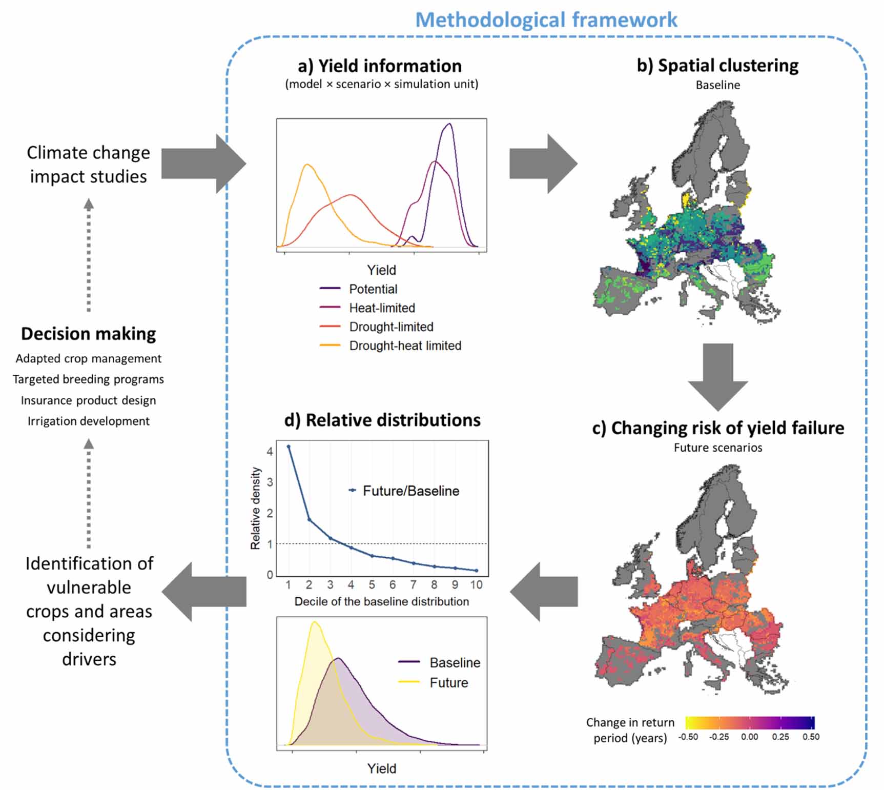
An overview of the methodological steps to evaluate the changes in risk of yield failure and in the underlying yield distributions under climate change is presented in figure 1. First (figure 1(a)), simulations results from an ensemble of crop and climate models were processed (figure 1(a)) as described in section 2.2. The second methodological step involved grouping (figure 1(b); section 2.3) the simulation results into spatial clusters based on yields in the baseline scenario and stress intensity. The clustering was performed to provide discrete units for the subsequent analysis and to provide large enough sample of data to apply the relative distribution methods. In the third step, yield failure under baseline climate (as defined in section 2.4) and the relative change in return periods between successive yield failures under climate change scenarios were quantified (figure 1(c); results presented in section 3.2). The next methodological step was the application of the relative distributions (figure 1(d); section 2.5) to assess which aspects of the underlying yield distributions were driving the changed yield failure frequencies. This is a non-parametric framework that summarizes the differences between two distributions (here crop yields under baseline climate and climate change scenarios) with a single curve, highlighting differences occurring throughout the entire range of values (simulated yields in this study). The relevant features of the source dataset used as case study are described in section 2.6.
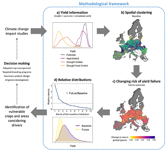
Figure 1. Schematic representation of the methodological framework to analyze the evolution of yield failure frequency. Input data produced by simulation experiments (a) are used to define spatial clusters in the baseline scenario (b) and to assess changes in yield failure frequency (c). Relative distribution methods (d) are applied to study changes in simulated yield distributions. Solid and dashed arrows represent data and information flows, respectively.
Download figure:
Standard image High-resolution image2.2. Crop yield simulations and drivers
Data used in this analysis were time series of crop yields simulated by an ensemble of crop and climate models under potential (YPOT), heat-limited (YHL), drought-limited (YWL), and drought-heat limited (YWHL) conditions under baseline climate and climate change scenarios across a grid of simulation units (see section 2.6). Under any growing condition, 30 year time series of yields were available in each simulation unit and climate scenario for any combination of crop × climate model. Heat and drought limited yields were related to potential yields in the baseline climate scenario to produce time series of stress indices calculated according to equation (1):
where StressIndex and correspond to HS (for heat stress) or WS (for drought stress), Ylim either to YHL (for heat stress) or YWL (for drought), i is the simulation unit, t the year and m either the crop model. These indices represent the independent contribution of heat and drought to the yield gap between YPOT and YWHL. Stress indices range from 0 (indicating no stress) to 1 (no yield at harvest due to the stress).
2.3. Spatial clustering
For each crop model, the average value of the time series of YPOT, YWHL, HS and WS were used to characterize the typical production situation in each simulation unit under baseline climate. Such indicators were selected as the measures summarizing the yield potential and main yield drivers accounted for by the models, i.e. potential yields determined by CO2 assimilation and conversion as modulated by solar radiation and temperature regimes for a given variety (YPOT), the independent influence of water stress (WS) and heat stress (HS), and finally, water-heat limited yields as the outcome of both stressors (YWHL). For each of these measures, the median across crop models was used to characterize the ensemble response in each simulation unit (equation (2)). Considering the spread across different crop models, the median was preferred over the average for its robustness against outliers
where EEx is the ensemble estimate, t the year in the time series, x is either YWHL, YPOT, WS or HS, and m the models in the set of crop models M used in this study. Simulation units were then clustered using ensemble estimates of YWHL, YPOT, WS and HS in the baseline scenario, identifying areas with homogenous yields and drivers (i.e. simulation units falling in the same category for the four ensemble estimates). YWHL, YPOT and WS were classified based on their range simulated across the study area as low (lower quartile), medium (interquartile range) or high (upper quartile); HS, due to less variation, was divided into two classes only (low and medium-low). Clustering was performed to provide an overview of the emergent spatial patterns of yields and the yield drivers in the baseline while generating large enough samples of yield data for the application of relative distribution methods (section 2.5).
2.4. Yield failures
A yield failure was counted when simulated yield was lower than a threshold relative to the Olympic average yield of the previous five-years (Webber et al 2020b), i.e. the average yield obtained ignoring the highest and lowest yields in the preceding five-year period. Olympic averages, as commonly used by the insurance industry and governments to define yield failures (EC 2017), were used to ensure the definition of yield failures were not biased by the occurrence of exceptionally good or bad yields in the recent past. The definition of failure follows European guidelines (EC 2017) that identify a natural or other disaster by a production loss, which exceeds 30% of the average of production. Since a lower threshold for crop failure may be more appropriate for risk analysis at aggregate scales (Finger 2012, Heimfarth et al 2012, Webber et al 2016, Ben-Ari et al 2018), we assumed the threshold of 15% as a reference for the current study. The frequency of yield failure in each simulation unit and scenario was quantified as the average return period (RF,) between successive failures. For each simulation unit, crop, crop model and climate scenario, RF was estimated using time series of YWHL (thus accounting for the joint effects of drought and heat) to count the number of occurrences of a failure. The model ensemble median of RF was used as a risk indicator for each simulation unit under baseline and climate change scenarios (independently for each RCP). The ensemble estimates of RF were further aggregated at the level of spatial clusters (equation (3)) based on current production area (MIRCA2000; Portmann et al 2010):
where RFE is the ensemble estimate of the return period of a failure, w the fraction of the production area in the simulation unit relative to the total area in the spatial cluster (cl), i the simulation unit within the cluster, and s the climate scenario. To explore the uncertainty across models, the ensemble median of RF was calculated separately for (a) the pool of all the crop and climate models, (b) individual crop models (median across climate models) and (c) individual climate models (as the median across crop models).
2.5. Assessing distributional yield changes under climate change
Changes in crop yields between baseline and climate scenarios were quantified for YWHL at the level of spatial clusters using the relative distribution methods, a set of non-parametric statistical approaches developed by Handcock and Morris (1998, 1999). The relative distribution methods compare two populations (respectively 'reference' and 'comparison') based on the fraction of the comparison distribution that fall in each quantile of the reference one. This allows to locate and identify the changes occurred across the entire distribution between the two populations. Differences are encoded by a single line, i.e. the relative density. When there are no changes between the two distributions, the relative density equals to 1 for all quantiles. Values higher (lower) than 1 indicate an increase (decrease) share of yields in the comparison distribution at the level identified by the rth quantile of the reference distribution. Differences due to changes in location (mean or median) can be isolated from those involving the shape of the distribution and quantified by summary measures (for more details, see supplementary S1 (available online at stacks.iop.org/ERL/16/104033/mmedia)). In this study, yields in the baseline climate and under climate change scenarios were taken as the reference and comparison populations, respectively. The analysis was conducted in R (R Core Team 2019) using the package 'reldist' (Handcock 2016).
Relative densities were evaluated within each spatial cluster for all the combinations crop model × climate scenario by pooling YWHL from all simulation units of the cluster. Current production areas (MIRCA2000; Portmann et al 2010) within the simulation units were used as weights for both the reference and comparison population. Data limitation prevented to evaluate the relative distribution at the scale of the single simulation unit, where data were not available for each quantile of the distribution. The choice of clustering simulation units was a pragmatic solution to reach the recommended minimum sample size (100–1000 observations; Handcock and Morris 1998), but constrained the resolution of the analysis to an aggregate level. For any combination of cluster × climate change scenario, the relative density at each decile of the reference population was calculated separately for (a) the pool of all the crop and climate models, (b) individual crop models (median across climate models) and (c) individual climate models (as the median across crop models). This allowed to explore the uncertainty in the relative density due to crop and climate models. The main patterns (types) of the changes in yield distributions across the study area and the climate change scenarios were identified applying hierarchical clustering (Suzuki et al 2019) to the ensemble estimates based on all crop and climate models of relative density.
2.6. Data source
The data for the current analysis were retrieved from Webber et al (2020a; doi: 10.4228/ZALF.DK.88). This dataset consists of an ensemble of eight crop models accounting for the impact of drought and heat stress on wheat and maize production (supplementary S2). In the study by Webber et al (2018), drought and heat stresses were quantified as the reduction of crop yield resulting respectively from water deficit during the crop cycle and periods of high temperature experienced around flowering and/or seed set. Gridded simulations (25 km horizontal resolution) covering the land area across the EU-27 (8157 simulation units) were available in the source dataset for baseline scenario (1981–2010) and future climate scenarios (2040–2069) for three RCPs (RCP 2.6, 4.5 and 8.5). The climate projections were available for five climate models (General Circulation Models, GCMs) under two forcing scenarios RCP 4.5 and 8.5, and two climate models under RCP 2.6. For each simulation unit and climate scenario (i.e. the combination of GCM × RCP), treatments were simulated for potential, heat-limited, drought-limited and drought-heat limited crop yields (supplementary S2). Full irrigation was simulated for potential and heat limited simulations, whereas under drought treatments crops were rainfed. To simulate yields without effects of heat stress (for potential and drought-limited treatments), modelers either switched off heat stress routines or set threshold temperature limits very high such that no heat stress damage was simulated. In all simulations, soil water content was re-initialized at sowing, and nitrogen was not considered as a limiting factor. Observed sowing, flowering and harvest dates were taken from the Eurostat (Eurostat, http://ec.europa.eu/eurostat/web/main) and then aggregated to the level of 1 of 13 agro-environmental zones across Europe (Metzger et al 2005) following the procedure reported in Zhao et al (2015) and Webber et al (2015). These phenology data were then resampled to the level of the simulation unit and used with simulation unit specific climate data in the baseline conditions to calibrate crop phenology parameters. For the climate change scenarios, simulations were available for baseline [CO2] (360 ppm) and elevated [CO2] of 442 ppm (RCP 2.6), 499 ppm (RCP 4.5) and 571 ppm (RCP 8.5). For the current analysis, we used simulated heat stress with canopy temperature, as this is considered more appropriate, although for two models only simulations using air temperature were available. For future scenarios, only simulations with elevated [CO2] were considered. The current analysis was restricted to rainfed cropping systems, i.e. simulation units characterized by at least 500 ha of rainfed area based on the MIRCA2000 global data set on crop area (Portmann et al 2010).
3. Results
3.1. Spatial clusters under baseline climate
When considering the range of variation of YWHL, YPOT, WS and HS, a total of 47 clusters were identified for maize and wheat, forming the basis of subsequent analysis (figure 2). Some common features arose between the two crops across Europe. Areas where both YWHL and YPOT were in the high range (i.e. clusters with 'HH' as the first two letters of the cluster name in figure 2) were found in France for maize (in the West) and wheat (North-West and Center). In wheat, such cluster reached areas scattered throughout Italy and Spain. However, a major portion of Spain, as well as part of the Mediterranean basin, were characterized by areas with the highest potential yields and intermediate to high levels of drought stress, as illustrated by the larger extent of clusters 'LH' (first two letters code) for both crops and 'MH' for wheat compared to 'HH' (figure 2). Conversely, large areas in Central and Northern Europe displayed intermediate and high YWHL, and a smaller difference between YWHL and YPOT due to a relatively lower impact of drought. On the other hand, areas in Northern Europe (Scandinavian countries for wheat and mainly Denmark for maize) displayed low yields both in potential and actual conditions (clusters 'LL' in figure 2), indicating thermal and solar radiation regimes as main limiting factors for crop growth. In both crops, the magnitude of heat stress was limited when compared to drought stress.
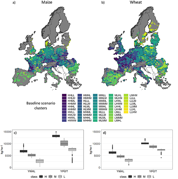
Figure 2. Spatial clusters of ensemble estimates of drought-heat limited yield (YWHL), potential yield (YPOT), drought stress (WS) and heat stress (HS) for maize (a) and wheat (b). The grey area represents simulation units excluded from the current study. Cluster names indicate the category of the four ensemble estimates in the simulation unit, ordered as follows: YWHL (first letter), YPOT (second letter), WS (third letter), and HS (last letter). High ('H', upper quartile), medium ('M', interquartile) and low ('L', lower quartile) categories are identified based on the range of variation of the ensemble estimates in the baseline scenario across the study area. Panels (c) (maize) and d (wheat) report the ranges for YWHL and YPOT.
Download figure:
Standard image High-resolution image3.2. Yield failure frequency changes
The return period of failures from drought and heat stress in the baseline climate scenario ranged from about 2.1–3.6 years for maize, and between 2.5 and 3.6 years for wheat when aggregated for the spatial clusters identified (figure 3, supplementary S3). In both crops, ensemble estimates of return period decreased while moving from clusters characterized by higher yields and limited drought stress to the ones with lower yields and greater stress. As a result, a North-South gradient was present, with Southern Europe mostly characterized by lower YWHL and shorter yield failure return periods.
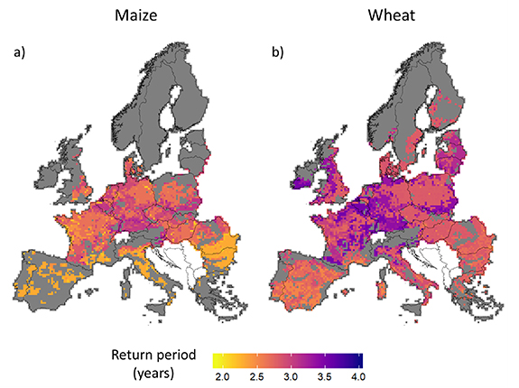
Figure 3. Ensemble estimates of return period of a failure for maize (a) and wheat (b) in the baseline climate scenario across the clusters identified. The grey area indicates simulation units excluded from the current study.
Download figure:
Standard image High-resolution imageUnder climate change scenarios, shorter return periods for crop failure were observed for maize, as opposed to the generally longer return periods for wheat. Under limited climate forcing, wheat displayed a mixed response, with shortening and increasing return periods almost equally represented across the study area. The magnitude of the change in return period of a failure was RCP-dependent, especially for wheat. (figures 4 and 5). Regardless the RCP considered, failures that became more frequent were more pronounced for maize in the areas characterized by the highest yields in the baseline scenario (i.e. clusters H.YWHL-H.YPOT, H.YWHL-M.YPOT and H.YWHL-L.YPOT in figure 2). A significant negative relationship between baseline return period and its change under all the RCP scenarios was observed for maize (supplementary S4). For wheat, the high yielding clusters in the baseline scenario were among the areas that mostly benefited from the increase in return periods. A comparable increase in the return period was observed, for wheat, also in the clusters characterized by low yield and low potential in the baseline scenario (i.e. L.YWHL-L.YPOT in figure 2), particularly under RCPs 4.5 and 8.5 (figures 4(d) and (f)). The response described for the ensemble of all crop and climate models (figure 5(a)) was consistent with the one from individual climate models (figure 5(c)). The response from individual crop models, on the other hand, was more uncertain and characterized by less agreement in the sign of the change in return period of yield failures among ensemble members (figure 5(b)).
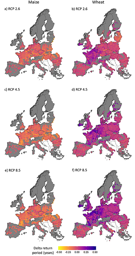
Figure 4. Ensemble estimates of changes in return period of a failure for maize ((a), (c), (e)) and wheat ((b), (d), (f)) under different climate change scenario ((a), (b): RCP 2.6; (c), (d): RCP 4.5; (e), (f): RCP 8.5) across the clusters identified. In each cluster, delta return period is the difference between return period of yield failure under climate change and baseline scenarios. The grey area indicates simulation units excluded from the current study.
Download figure:
Standard image High-resolution image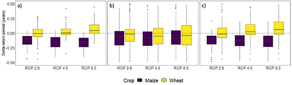
Figure 5. Range of variation of the change in return period of yield failure across the clusters identified and for the different climate scenarios (RCP) considered. In each cluster, delta return period is the difference between return period of yield failure under climate change and baseline scenarios. In the three panels, the deltas are calculated respectively for the ensemble of all crop and climate models (a), individual crop models (b) and individual climate models (c).
Download figure:
Standard image High-resolution image3.3. Relative distribution analysis
Our analysis highlighted diverging responses of the yield distributions (YWHL) of maize and wheat to climate change (figure 6). Depending on the crop, the relative density is greater than 1 at the opposite ends of the distributions, depicting a general increase of probability of low yields for maize (figure 6(a)) and of high yields for wheat (figure 6(c)) under climate change scenarios. Three main response types were identified for each crop across the spatial clusters covering the study area. For maize, an increase in the frequency of yields in the lowest deciles was projected for all types, in particular for extreme low yields. The regions least negatively affected by climate change (corresponding to 'low-neg' type in figure 6(a)) displayed relative densities between 1 and 1.3 for yield levels below the median baseline yield level. An almost symmetric decrease in the relative densities for high yields was observed. The other two types identified for maize (i.e. 'mid-neg' and 'hi-neg', increasingly affected by climate change) followed a similar pattern, but with more dramatic variations at the extremes (figure 6(a)). For all the types, the overall relative distribution resulted from the combined effects of a location (mean) shift toward lower values and a change in shape that reduced the frequency of extreme values at both ends of the distribution. The changes in shape partially mitigated the location effect for low yields while further reducing the occurrence of yields in the highest deciles (supplementary S5). While moving from areas less negatively affected by climate change (type 'low-neg') to areas displaying relative distributions of type 'mid-neg' and 'hi-neg', the contribution of location changes to the overall relative distribution increased while the shape effect decreased (figure 6(b)). The relative distributions from individual crop and climate models were consistent with those outlined by the ensemble median for maize. Crop and climate models contributed to a similar extent to uncertainty, which was more marked at the lowest and highest deciles (figures 7(a)–(c)).

Figure 6. Types of relative distributions of maize ((a), (b)) and wheat ((c), (d)) yields between baseline (reference population) and climate change (comparison population) scenarios, based on the ensemble median of crop and climate models. The labels identify the magnitude and direction of the impact of climate change. For maize, the impact is increasingly negative for types 'low-neg', 'mid-neg' and 'hi-neg'. For wheat, the impact is increasingly positive for types 'low-pos', 'mid-pos' and 'hi-pos'. The overall relative distribution ((a), (c)) is decomposed into location and shape components ((b), (d)).
Download figure:
Standard image High-resolution image
Figure 7. Range of relative distributions for individual crop models (orange shade) and climate models (violet shade). Solid lines identify the interquartile range, whereas shaded areas extend to 1.5 times the interquartile range. Panels report the main types of relative distributions for maize (a)–(c) and wheat (d)–(f) ordered according to the magnitude and direction of the impact of climate change. For maize, the impact is increasingly negative for types 'low-neg', 'mid-neg' and 'hi-neg'. For wheat, the impact is increasingly positive for types 'low-pos', 'mid-pos' and 'hi-pos'.
Download figure:
Standard image High-resolution imageFor maize, the three types of relative distributions had a different extent and spatial allocation across Europe depending on the RCP (figure 8). The least negative response of yield distribution to climate change ('low-neg') was prominent under RCP 2.6 (covering about 70% of the total rainfed area), with medium and high impact responses relegated to a transect crossing Central Europe (with a coverage of 24% and 6%, respectively; figure 8(a)). Under higher forcing scenarios, high impact responses covered the majority of the land area used for rainfed maize production (figures 8(c) and (e)). The'mid-neg' and 'high-neg' responses covered 38% and 30% of the total rainfed area in Europe under RCP 4.5. The respective values for RCP 8.5 were 46% and 23%. A 'low-neg' response generally occurred in areas characterized in the baseline scenario by more frequent yield failures and medium to low drought-heat limited yields, whereas 'mid-neg' and 'high-neg' responses were associated with more favorable conditions in the baseline (longer return periods for yield failure and higher drought-heat limited yield). Under higher forcing scenarios (RCPs 4.5 and 8.5), the 'mid-neg' and 'high-neg' responses extended into less favorable areas. Regardless the climate scenario, 'low-neg' response was associated with a limited shortening of the return period of yield failures, whereas higher impact responses were associated with increased shortening of the return period for a yield failure (supplementary S6).

Figure 8. Spatial distribution of the types of relative distribution identified under for maize ((a), (c), (e) respectively for RCP 2.6, 4.5 and 8.5) and wheat ((b), (d), (f) respectively for RCP 2.6, 4.5 and 8.5). Total rainfed area is aggregated for each type. The grey area indicates simulation units excluded from the current study. The labels identify the magnitude and direction of the impact of climate change. For maize, the impact is increasingly negative for types 'low-neg', 'mid-neg' and 'hi-neg'. For wheat, the impact is increasingly positive for types 'low-pos', 'mid-pos' and 'hi-pos'.
Download figure:
Standard image High-resolution image
Relative distributions of wheat yields showed distinct responses compared to maize. Under RCP 4.5, the probability of high yields (r ⩾ 0.8) increased, whereas the probability of lower yields decreased. Three response types were identified based on the magnitude of such changes (figure 6(c)). A response 'hi-pos' identified areas where crop yields benefited the most from climate change, with a relative density of yields in the top decile just above 2.5 and a decrease (with relative density of about 0.6) in yields in the low end of the distribution. The other types displayed relative densities in the top decile around 1.7 ('mid-pos') and 1.3 ('low-pos'), and almost no changes in the probability of extreme low yields for 'low-pos'. For all the response types, distributional differences resulted from a shift in the mean towards higher values combined with a change of shape that tended to increase frequency of extreme values at both ends (supplementary S5). For 'high-pos' response, the influence of the location effect dominated the overall distributional differences, whereas for the other types a more balanced contribution of location and shape changes was observed (figure 6(d)). The uncertainties in the relative distributions were less marked for wheat than for maize, with differences among crop models playing a major role (figures 7(d)–(f)). A 'low-pos' response was the most widely represented under RCP 2.6 (98% of the total rainfed area; figure 8(b)) and RCP 4.5 (79%; figure 8(d)), outlining a widespread mild positive impact of climate change on simulated wheat yields. Under higher forcing scenarios, the extent of 'mid-pos' response increased (21% and 67% of the area under RCP 4.5 and 8.5, respectively; figures 8(d) and (f)). A 'high-pos' response to climate change was observed almost only under RCP 8.5 (figure 8(f)), where it covered about 13% of the land area, mainly in Central and Northern Europe. Under RCP 4.5, a 'low-pos' response was mainly associated with the spatial clusters displaying the highest yields in the baseline scenario, whereas a 'mid-pos' response was mainly related to clusters with medium and low yield levels in the baseline. Such association not apparent under RCP 2.6 and 8.5. In contrast with maize, wheat did not display—across RCPs—a consistent relation between response type and the magnitude of the change of the return period for a yield failure (supplementary S6).
4. Discussion
4.1. Significance and implications
Climate change is expected to increase yield variability and the risk of crop yield failures, representing a significant challenge to food security (Wheeler and Von Braun 2013). While crop modeling has provided insights into the expected changes in average yield levels with future climate change (Challinor et al 2014, Deryng et al 2014, Rosenzweig et al 2014, Schleussner et al 2018, Webber et al 2018), few studies have considered the projected shift of yield distributions and implications for yield failure frequencies (e.g. Challinor et al 2010, Webber et al 2016, Faye et al 2018). This is particularly relevant for many currently low income world regions at low latitudes where large negative climate impacts are projected (Rosenzweig et al 2014). In these regions, climate risk is linked to the extent and persistence of rural poverty, with shocks eroding productive assets of smallholder farmers, limiting investments in agriculture and the adoption of improved technologies (Hansen et al 2019). As climate-induced yield variability often increases with intensification (Faye et al 2018, Müller et al 2018), climate risk is likely to further constrain decisions to intensify production (Hansen et al 2019, Benami et al 2021). In the context of an increased climate-driven uncertainty, understanding what drives the changes along the yield distributions (and the implications for yield failures) will contribute to the design of improved adaptation measures, targeting the stability of crop yields (e.g. investments in irrigation infrastructure or crop breeding) and of farmers' income (e.g. subsidizing insurance products).
In this context, here we presented an approach to quantify how yield distributions and the associated risk of yield failures change using an ensemble of crop and climate models. We demonstrated the approach for Europe, where we could take advantage of an existing dataset for the case of two important cereal crops. We present and discuss the results as a demonstration of the methodology, illustrating the types of information that can be provided, including a quantification of the uncertainties. For this test case, our results highlighted a general increase in risk of yield failure for maize under climate change across Europe, particularly marked in areas characterized in the baseline scenario by relatively high yields and a low risk of failure. The increase of the risk of yield failures was associated with a shift of the yield distribution towards lower values and changes in shape of the distribution that further reduced the frequency of high yields. The adaptation potential deriving from the adoption of later maturity hybrids appeared in this case limited, as drought stress already intensified despite the shorter crop cycle (Webber et al 2018). The demonstration case illustrated a different picture for wheat: the risk of yield failure generally declined under future scenarios, accompanied by a shift of the distribution towards higher values and a change in shape increasing the frequency of extreme values at both ends of the distribution. The differential patterns of risk of failure emerging for maize and wheat may inform adaptation strategies related to the regional allocation of crops (Bindi and Olesen 2011, Zimmermann et al 2017). The availability of simulation results from different crop and climate models provides the opportunity of quantifying the model uncertainties in the definition of the spatial clusters, in the changes in risk of yield failure and in the relative distributions. In the case study, the exploration of uncertainties revealed that while the relative distributions projected by different crop and climate models were consistent, uncertainties from crop models could hamper the identification of the sign of changes in the risk of yield failures.
While our intention is to demonstrate the risk assessment method, our results are consistent with studies looking at the drivers of yield change across Europe. The shift of wheat yield distributions towards higher values was explained by the fertilization effect of increased atmospheric CO2 concentrations (Webber et al 2018). The CO2 effect may also explain the discrepancy between the projected changes in wheat yields and the large negative impacts on wheat throughout Europe outlined by statistical models (e.g. Moore and Lobell 2014, Gammans et al 2017). When removing this effect, the different methods produced similar estimates of climate change impact on wheat yields (Liu et al 2016). In our case study, removing the CO2 effect led to an increased frequency of low yields for wheat, particularly in the lowest deciles (results not shown).
4.2. Relative distributions: opportunities and challenges
Though empirical modeling of the yield probability distribution has been performed for economic analysis (Tack et al 2012, Malikov et al 2020, Ramsey 2020), the majority of studies assessing climate change impact studies have focused on the mean effects of climate change, providing relatively limited insight into the distributional heterogeneity in climate change effects. In this study, climate change impacts were assessed for yield distributions using the relative distribution method. In turn, changes in the frequency of yield failure were related to changes in the distribution of yields.
The relative distribution method is suited to the analysis of changing risk under climate change, where different aspects of the yield distributions may be affected (e.g. as a result of shifts in mean and increased probability of extreme values). Moreover, as the shape of the yield distribution can be skewed and interact significantly with management factors (Day 1965), traditional parametric methods for the representation of yield distributions may introduce bias in the analysis of crop yields (Rötter et al 1997). The absence of parametric assumptions, conversely, makes relative distribution ideal for the analysis of crop yields. While relative distributions can quantify differences occurring at any quantile of the yield distribution, the method also allow to summarize differences into two basic components, i.e. changes in location (mean or median) and in shape (a general concept comprising higher moments of the distribution). Combined with the analyses of drivers of changes in crop yields (Webber et al 2018), this could quantify the influence of climate drivers on specific changes in yield distribution critical for yield failure, highlighting the causes of the risk associated with the cultivation of a crop in vulnerable areas. In this study, we focused on the joint contribution of drought and heat stress under elevated atmospheric CO2 concentrations. However, the relative distribution could be applied to different production levels (e.g. potential, drought limited, heat limited, drought-heat limited, with and without elevated CO2 concentrations) to gain insights in the effect of various drivers and their interaction along the entire yield distribution under climate change.
A main challenge in applying relative distributions to the analysis of crop yields is the need of large enough datasets to provide reliable estimates of the changes occurring along the entire yield distribution. To this end, in our study data from different simulation units had to be pooled, limiting the resolution of the analysis as adaptation studies must clearly be based on data at a higher spatial resolution. Nevertheless, our intention with the study was to provide a proof of concept for the use of relative distributions, showing their relevance for policy and insurance by outlining the broad patterns of changes in risk of yield failure under climate change. While not ideal due to potentially confounding effects of spatial and temporal variability, our method to define relatively homogeneous clusters with respect to yield level and drivers and the fact that, within each cluster, spatial variability had a similar influence on the reference and comparison distributions limits such problem in our study, focused on assessing how the importance of heat, CO2 and drought influence heat and water limited yields. Such shortcomings could be avoided by using a different set of climate data as input for the crop models. In this study, a single climate series (30 years) was used as baseline for the generation of future scenarios. A larger sampling of input data series (e.g. produced by weather generators) would make the spatial clustering unnecessary for applying the relative distributions, that could be evaluated at a disaggregate level. Ideal sets of climate data for the purpose would be the super-ensembles developed by the HAPPI project (www.happimip.org/about/), which provides bias corrected climate model outputs with a focus on global warming impacts of 1.5 °C and 2 °C increase above pre-industrial level. These data series are specifically developed for their use as input to impact models, enabling an analysis of the relative risks of low-probability extreme weather events (Mitchell et al 2017).
4.3. Limitations of the study
The study relies on the accuracy of crop models' estimates of yield distributions. Crop models are constructed to consider relevant yield determining factors and often further calibrated to display a consistent response to variables that are not explicitly captured in the modeled processes. Studies conducted at field scale generally make use of extensive validation to ensure crop models can explain a large portion of the observed yield variability. For applications at larger scales (e.g. regional and global studies), validation with observed data is limited by the use of aggregated yield statistics as reference values (Müller et al 2017, Guarin et al 2020) and by the uncertainties in crop management. Here, the analysis of yield anomalies across NUTS2 districts revealed a tendency of the models to overestimate baseline risk of failure across Europe (supplementary S7). This is partially expected for large scale simulations, since the specification of management, soil and varieties at an aggregate level may underrepresent the heterogeneity of the real systems that acts to buffer the effects of shocks. On the other hand, important drivers of relatively localized low yield levels related to excessive rainfall (e.g. delayed operations, poor emergence, waterlogging, disease, nitrogen leaching or harvest losses), frost damage or lodging are difficult to consider in crop models simulations intended for large area application (Ewert et al 2015). As a result, simulated yields when these conditions prevail is likely to be overestimated, leading in turn to an overestimation of yield variability driven by heat and drought stress. In fact, as many crop models applied in large area studies capture only weather conditions related to temperature and drought as drivers of interannual yield variability, missing other weather and management factors which act to lower yields in good years, the end result is that simulated yield variability is often overestimated. Finally, some models that did not leverage canopy temperature might have underperformed in the simulation of heat stress. However, we opted to keep these models in the ensemble to be comparable to the study of Webber et al (2018). These authors reported that effects on phenology, CO2 fertilization and drought stress had a comparatively larger effect on yield changes, justifying keeping other models to capture more process uncertainty.
The evaluation of yield failure at farm level remains challenging, since the finest scale allowed by input data (25 km resolution) provides information at an aggregate level. Due to the underlying variability of soil and weather conditions, as well as farmers' management practices, yield variability at the farm level can be significantly different than at aggregate level (Finger 2012), introducing a bias in yield risk analysis that needs to be considered in the design of adaptation measures at the aggregate level (Heimfarth et al 2012). Scaling also questions the appropriate threshold for assessing yield failure. A common threshold at farm level is 30% for crop failure, but the reduction of yield variability with aggregation calls for the application of a lower threshold. Quantifying the scaling errors associated with the choice of the threshold requires yield data at the farm level that were not available. However, Webber et al (2020b) observed that the threshold had very small effect on the identification of the years with the most widespread occurrence of failures for different crops in Germany. In this study, a relatively low threshold (15%) combined with the tendency of the models to overestimate the frequency of yield failures (supplementary S7) probably explains the high frequency of failures observed across climate scenarios.
5. Conclusions
This work aimed at providing a methodology to assess how climate change may translate into changes in risk of yield failures. Given the role of yield distributions in shaping the risk profile, the analysis of relative distributions was a cornerstone of the present work. The relative distribution methods, widely used in social sciences, were applied here for the first time in crop modeling. Relative distributions were used to study the changes occurring across the entire yield distribution under climate change, providing insights that are missed by common analyses of average shifts in crop yields. As a case study, we applied the method to assess changing patterns of the risk of yield failure expected across Europe for maize and wheat under three climate change scenarios, using published results from an ensemble of crop models. The method as applied revealed diverging patterns of changes in yield distribution under climate change for the two crops, associated with opposite responses in terms of risk of yield failure. For maize, a shift of the yield distribution towards lower yields and changes in shape of the distribution that reduced the frequency of high yields determined an increased frequency of yield failure under climate change. Such pattern emerged especially in areas characterized by higher yields and lower frequency of yield failure, and it became widespread across Europe under higher radiative forcing scenarios. For wheat, yield failures generally declined under future scenarios, with a shift of the distribution towards higher yields and a change in shape increasing the frequency of extreme yields favored by increased CO2 concentrations. Our test exercise revealed a number of challenges to be overcome in the future applications of the method. As the relative distributions require a larger number of yields per location than were available in the 30 year times series per simulation unit, we performed a clustering to increase our sample size, constraining the scale of the analysis to an aggregate level. Finally, for reliable risk assessments, modeling efforts need to be made to represent the effects of multiple stresses determining yield failures.
Acknowledgments
T S, H W and F E received funding from the International Wheat Yield Partnership (IWYP115 Project). H W acknowledges support from the FACCE JPI MACSUR project through the German Federal Ministry of Food and Agriculture (2815ERA01J). J E O was funded from the FACCE MACSUR project by Innovation Fund Denmark and by the SustES project—Adaptation strategies for sustainable ecosystem services and food security under adverse environmental conditions (CZ.02.1.01/0.0/0.0/16_019/0000797), which supported K C K as well. Rothamsted Research receives grant-aided support from the Biotechnology and Biological Sciences Research Council (BBSRC) through Designing Future Wheat [BB/P016855/1] and Achieving Sustainable Agricultural Systems [NE/N018125/1]. P M and L M acknowledge support from the FACCE JPI MACSUR project (031A103B) through the metaprogram Adaptation of Agriculture and Forests to Climate Change (AAFCC) of the Franch National Research Institute for Agriculture, Food and Environment (INRAE). F E acknowledges support from the German Federal Ministry of Food and Agriculture (BMEL) through the Federal Office for Agriculture and Food (BLE), (2851ERA01J) for FACCE MACSUR, the German Research Foundation under Germany's Excellence Strategy, EXC-2070—390732324—PhenoRob.
Data availability statement
The data that support the findings of this study are available upon reasonable request from the authors.