


Abstract
Radial transport of runaway electrons (REs) in tokamaks is affected by the presence of magnetic perturbations, either caused by internal magnetohydrodynamic instabilities or induced by external coils. The magnetic field configuration inside the plasma volume consists in general of intact magnetic surfaces alternated with magnetic islands and stochastic layers, which make the usual diffusive approach, based on the Rechester–Rosenbluth formula, inadequate to the study of transport. Here the fractional diffusion approach is employed to model RE transport in presence of intrinsic magnetic perturbations (magnetic islands) in the flat-top phase of RE-dedicated discharges on COMPASS tokamak. The character of RE transport is found to be subdiffusive. The degree of subdiffusion is evaluated by running simulations with the ORBIT code and a time-fractional diffusion equation is applied to calculate the time evolution of RE particle number. The results are compared with the observed RE losses, estimated from the time integrated neutron signal.
Export citation and abstract BibTeX RIS

Original content from this work may be used under the terms of the Creative Commons Attribution 4.0 license. Any further distribution of this work must maintain attribution to the author(s) and the title of the work, journal citation and DOI.
1. Introduction
Large toroidal electric fields following a disruption event are capable of accelerating a large fraction of the electrons to relativistic energies. These energetic electrons are called 'runaway electrons' (REs) and they represent one of the main obstacles to the successful operation of ITER [1]. RE dynamics and transport is affected by the presence of magnetic perturbations, either caused by internal magnetohydrodynamic (MHD) activity, such as tearing modes (TMs) or externally generated resonant magnetic perturbations (RMPs). The use of RMPs proved to affect RE losses [2–4]. Use of RMPs proved to enhance the electron drift orbits, thus leading to larger RE losses, although the external perturbations do not necessarily cause the creation of stochastic regions. During plasma disruptions, the structure of magnetic surfaces is broken and large regions of stochastic magnetic field are created. This would cause most of the particles to rapidly leave the plasma volume, but the rapidly reforming magnetic flux tubes are able to trap REs for a long time [5]. JOREK simulations [6] and models based on externally imposed magnetic perturbations [7] indicate that magnetic field lines fail to intercept the chamber walls in the case of surfaces near the magnetic axis and inside magnetic islands. Integrations of relativistic electron trajectories show that the electrons can be confined in both these circumstances. The time scale of fast current relaxation, which take place in disruptions, was shown to be faster than predicted by resistive models, which means that magnetic surfaces heal fast enough for some of the REs to remain confined.
The evidence of a coupled dynamics of REs and magnetic islands was observed in the form of a correlation between the hard x ray (HXR) signals, or the Cherenkov signal, and the magnetic signals obtained by Mirnov pick-up coils [8, 9]. In particular, rotating magnetic islands were observed to cause a periodic modulation in the RE emission, visible in the HXR and in the Cherenkov signals. According to theoretical predictions [5], sufficiently large magnetic islands are capable of trapping energetic electrons, which are then accelerated by the electric field and reach high energies, or increase exponentially through the avalanche mechanism [10]. Internal MHD modes can grow and partially overlap, leading to the formation of large stochastic regions. The presence of partially broken magnetic surfaces and chains of magnetic islands makes the usual diffusive approach inadequate to the study of transport, and the fractional diffusion model should be used instead. In the reversed field pinch (RFX) in Padova, where large regions of chaotic magnetic field are observed in between magnetic islands, particle transport was evaluated and it was found to be subdiffusive [11]. The subdiffusive character of ion and electron transport was identified in different tokamak devices, with different amplitudes and spectra of magnetic perturbations [12].
In this paper we show that RE transport in COMPASS in the presence of small amplitude MHD perturbations turns out to be subdiffusive. This behavior is observed by performing particle simulations with the ORBIT code [13]. A fractional diffusion model is adopted to interpret the results and to evaluate the degree of subdiffusion. We observe that the long-term behavior of the RE losses follows an inverse-power law, which is in agreement with the predictions of the subdiffusive model. Slower-than-diffusive transport implies that REs can remain in the plasma volume longer than predicted by usual diffusive models, which might represent a serious issue for large devices such as ITER. The paper is organized as follows: in section 2 some experimental observations of REs in COMPASS are provided; in section 3 the main theoretical concepts concerning fractional transport are introduced; in section 4 the reconstruction of magnetic configuration inside the plasma is described; in section 5 the results of simulations with the ORBIT code on a circular COMPASS equilibrium are presented; in section 6 the numerical integration of the fractional diffusion equation is performed; in section 7 considerations on the energy dependence of the diffusion coefficient are made; in section 8 qualitative comparison of the numerical results with experimental measurements in COMPASS are performed; in section 9 the results are discussed and in section 10 conclusions are drawn.
2. Experimental measurements
REs have been studied in COMPASS both in quiescent low-density, circular discharges and in disruption-like scenarios induced by gas injection. The gas can be injected either by a piezoelectric valve or by a massive gas injection solenoid valve [14]. RE generation is favored by a small gas injection in the ramp-up phase of the current, while a second, larger gas puff is injected later to suppress the background plasma. The RE seed formation can be observed in the vertical electron cyclotron emission (ECE) or the unshielded HXR signal, which is proportional to the particle losses. The unshielded HXR signal evolves during the flat-top phase according to the evolution of the RE beam and can grow up to saturation after the disruption [8]. The flat-top phase is often characterized by the presence of some MHD activity, typically in the form of a slowly rotating (8–10 kHz) (2,1) magnetic island, visible in the magnetic signals collected by the Mirnov coils. The RE beam in the cold, post disruption plasma is visible as a long ramp-down of the current, the 'plateau'. The application of RMPs of different amplitude and phase in the flat-top phase proved to affect the RE suppression by changing the slope of the current (current decay rate) [2, 3]. An example of typical RE discharges in COMPASS is displayed in figure 1. Here the plasma current, the unshielded HXR signal and the two gas puffs applied in the early phase (D fueling) and in the late phase (Ar puff) of the discharge are displayed. The two discharges present different phases of MHD activity, visible as signals with different length and intensity in the spectrograms, which are associated with a modulated loss of electrons, visible in the unshielded HXR signal.

Figure 1. Comparison between two low-density, circular COMPASS discharges with a RE beam, whose presence is discernible from the unshielded HXR signal, associated with RE losses. The discharges are characterized by MHD activity, with frequencies in the order 5–10 kHz, visible as signals with different length and intensity in the spectrograms obtained from LFS midplane Mirnov coils.
Download figure:
Standard image High-resolution imageExperimentally, REs can be detected by synchrotron radiation detectors, photo-neutron and HXR detectors, Cherenkov and ECE [15] detectors. The magnetic perturbations present in the plasma volume can be studied by looking at the signal from Mirnov pick-up coils. The primary means of RE research at COMPASS relies on standard unshielded HXR diagnostics [8], based on a pair of NaI(Tl) scintillation detectors with photomultiplier tube and a composite scintillator, that was recently extended by CeBr3 detectors [16]. The set of magnetic diagnostics of COMPASS tokamak consists of three poloidal arrays of internal Mirnov pick-up coils at different toroidal positions covering all three components of magnetic field by 24 coils each, which allows the measurement of poloidal and toroidal mode numbers. Measurement of correlations between HXRs and magnetic signals from Mirnov coils provides evidence of a coupled dynamics of REs and TMs [8]. The HXR radiation is mainly generated in RE-wall and RE-impurity interactions. When the REs escape the plasma volume, they can hit the wall or the protection limiter. In the first case, it is a non-localized measurement because the radiation can be emitted in different points of the wall; in the second case, the source of radiation is localized. When the unshielded HXR signal is saturated, because of significant RE losses, a measure of the number of REs can be provided by the photo-neutron detector, which is adequately shielded.
3. Fractional transport
The magnetic configuration inside the plasma volume is in general constituted by partially broken magnetic surfaces, chains of magnetic islands and stochastic layers. The usual diffusive model, where the diffusion coefficient is provided by the Rechester–Rosenbluth (RR) formula [17], is strictly valid only for perfectly uniform magnetic chaos well above the stochastic threshold [18, 19]. This situation takes place usually just after a disruption, where the magnetic surfaces are rapidly broken because of the rapid growth and overlapping of MHD modes, triggered in a cascade process [20]. In the flat-top phase, where the plasma current is approximately constant and most of the magnetic surfaces are intact, the magnetic equilibrium can be perturbed by low-order MHD modes which can lead to the onset of magnetic islands, that persist for several ms before locking to error fields or being suppressed. Whether we are in a situation of mostly intact magnetic surfaces (flat-top) or in a mostly chaotic situation (post-disruption), the ordinary diffusive approach is not valid to describe the RE transport, and a fractional diffusion model should be used instead.
In the fractional diffusive regime, the mean square displacement of particle orbits grows with a fractional power of time,  , where Kp
is the fractional diffusion coefficient. The fractional exponent p is related to the Hurst exponent H by
, where Kp
is the fractional diffusion coefficient. The fractional exponent p is related to the Hurst exponent H by  , where
  , α and β being associated with the space and time behavior respectively, through the probability density distribution and the waiting time distribution [21]. Typically, the fractional exponent p is below one, which means that the regime of transport is subdiffusive. Fractional transport is characteristic of physical systems that exhibit spatial or temporal nonlocality (memory or long-term correlations [21, 22]). Subdiffusion has been found in different scenarios of anomalous transport in fusion plasmas, ranging from tracers in gyrokinetic simulations [23–25] to test-particle transport of thermal and energetic ions and electrons [11, 12, 26]. A typical value of subdiffusive exponent in these simulations is p ≈ 0.6, but values can range between 0.5 and unity [12]. This means that the particles will diffuse more slowly than in the classical diffusion case (p = 1), and a fraction of them can eventually be trapped for a long time before leaving the plasma volume.
To account for the fractional time dependence, the diffusion equation must be modified, and this can be achieved by replacing the ordinary time derivative with a fractional-order time derivative, which introduces a temporal non-locality in the system. The resulting equation is known as fractional kinetic equation (FKE) and was originally discussed by Zaslavsky [27, 28] and later applied to fusion plasmas [21, 29–31]. The implementation in terms of fractional derivatives makes the analogy with the ordinary diffusion equation more transparent, the disadvantage being that it violates causality by implying instantaneous propagation of information in the limit  . It is usually assumed thus that there exists a minimum time
  below which the FKE cannot be applied. In cylindrical geometry, the equation takes this form:
where  is the Caputo fractional derivative [32]:
where Γ is the Euler's gamma function, and the fractional diffusion coefficient Kp can be defined as:
The operation  represents the average over many different initial conditions for each radial position. The hypothesis behind equation (1) is that the fractional dependence falls only on time: a more general approach in terms of Montroll–Weiss equation [33], based on a microscopic formulation in terms of continuous time random walks, would allow to overcome this limitation by separating the space and time fractional dependences. Recently, an approach based on probability distribution functions has been used to simulate RE transport in the Madison symmetric torus [34]. A similar Montroll–Weiss approach to be used on COMPASS data is matter of a future work.
4. Reconstruction of magnetic configuration
The magnetic field configuration must be calculated properly to be supplied as input to ORBIT code. The poloidal mode number of the main MHD modes present in the plasma can be deduced by performing a phase-shift analysis on the magnetic signals from aligned Mirnov coils; a band-pass filter is applied to the raw Mirnov data to select the signal corresponding to the rotating MHD modes. The time integrated signal provides the magnetic field value at the edge of the plasma B(a): to obtain the radial profile of the different modes, the equation for tearing eigenmodes in cylindrical geometry must be numerically integrated:
where ψ is the perturbed poloidal magnetic flux. The boundary conditions at r = a are known:  and
and  ; the boundary condition in the origin is
  , while the first derivative
  is unknown. Equation (4) is solved by integrating forward from r = 0 up to the rational surface
  using a guess value for
  , the same equation is integrated backward from r = a to the rational surface
  with the boundary condition
  and a new value of
  is calculated by imposing that the solution is continuous at
  . The procedure is iterated until convergence is reached. The radial perturbation to the magnetic field can be computed as
  , where R is the major radius. An example of the spectrum of the perturbation for three low order modes is displayed in figure 2.

Figure 2. Magnetic perturbations  versus normalized minor radius
  corresponding to low order magnetic islands with different amplitudes.
Download figure:
Standard image High-resolution imageWe considered a circular plasma with minor radius a = 0.23 m, inverse aspect ratio ε = 0.3 and magnetic field on axis B = 1.15 T. The magnetic equilibrium was calculated analytically based on the prescribed q profile. The equilibrium and q profile for the considered case are displayed in figure 3. This represents a typical equilibrium employed in discharges performed during RE experiments in COMPASS.

Figure 3. Magnetic equilibrium (left) and q profile (right).
Download figure:
Standard image High-resolution image5. ORBIT simulations
To assess the character of RE transport in COMPASS, trajectories of energetic electrons were followed by performing simulations with the ORBIT code [13]. ORBIT calculates the guiding center particle trajectories by solving the Hamilton equations for the canonical moments Pθ
and Pζ
with the conjugated angles θ and ζ. An arbitrary spectrum of magnetic perturbations can be imposed over the equilibrium, so that different magnetic configurations can be explored. In the case of RE, relativistic effects become important since  , so in this case we employ the relativistic version of ORBIT developed in [35]. The algorithm for calculating the r.m.s. of jumps
 ![$\left\langle [r(t)-r(0)]^2 \right\rangle = \left\langle \Delta r^2 \right\rangle$](https://content.cld.iop.org/journals/0029-5515/64/1/016027/revision2/nfad0e31ieqn22.gif) used in [11, 12, 26] has been modified. Since the timestep for each particle is different, due to presence of the relativistic factor γ in the equations of motion,
used in [11, 12, 26] has been modified. Since the timestep for each particle is different, due to presence of the relativistic factor γ in the equations of motion,  is recorded together with the average particle time
  . In the same subroutine, the r.m.s. of the relativistic (canonical) momentum
  , where g is the covariant toroidal field in Boozer coordinates and
  is the parallel gyroradius, is recorded together with
  . To be able to extrapolate statistical results on the long-term particle behavior, 104 electrons were evolved for 104 toroidal turns, for different amplitudes of the MHD perturbation, corresponding to different levels of magnetic stochasticity, and for different energies of the electrons.
The spectrum of MHD perturbations was chosen in such a way to realistically reproduce a magnetic configuration that can take place during the flat-top phase of a RE discharge in COMPASS, with a few low-order magnetic islands with larger amplitude and other higher order modes with low amplitude, that can be triggered by poloidal coupling of the former ones. In particular, the primary modes have poloidal and toroidal mode numbers  equal to 3/2, 2/1 and 5/2, while the secondary modes correspond to
  equal to 5/4, 7/4 and 9/4. The perturbation to the magnetic field can be introduced in ORBIT in the form
  , where
  is the equilibrium magnetic field and
  is the perturbation spectrum [36]. The magnetic islands are assumed to be stationary, so that their rotation frequency is put to zero. In principle, each mode possesses a different phase
  : here for simplicity all the phases were assumed to be zero, which amounts to saying that the modes are phase-locked. Although phase differences between the different modes can affect their overlapping, we chose to examine only the effect of different amplitudes. The perturbation α can be calculated based on the magnetic flux perturbation obtained through the procedure described in the section above. The spectrum of modes considered in this study for a particular choice of their amplitude is shown in figure 4.
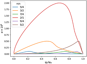
Figure 4. Magnetic perturbations α corresponding to low order magnetic islands with different amplitudes versus the poloidal flux normalized to its value at the edge of the plasma.
Download figure:
Standard image High-resolution imageTo explore different degrees of stochasticity, different amplitudes of the primary modes were considered, which leads to partial overlapping of the islands. The value of the magnetic perturbation measured in typical COMPASS discharges is in the order of  –
– , which corresponds to α ≈ 1–
 . The amplitude of all the modes was put to 10−5 in the small-amplitude case, with the exception of the mode 2/1 which was put to 10−4. In the large-amplitude case the amplitude of the 3/2 and 5/2 modes was put to
  , while the mode 2/1 was put to
  . The amplitude of the 2/1 mode was chosen to be a little larger than the experimentally observed values to amplify the mode overlapping; this partially overestimates particle transport but it does not change qualitatively the results. Different electron energies were considered to assess the energy-dependence of the diffusion coefficient. The chaos of magnetic field lines and of particle trajectories in the different configurations can be appreciated in figures 5 and 6.
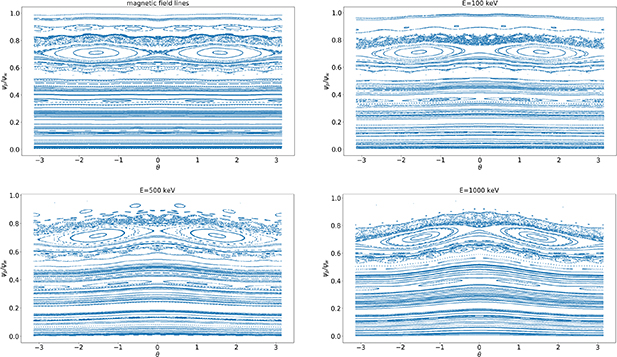
Figure 5. Poincaré sections of the magnetic field lines and of the particle trajectories in the  plane for the small amplitude case (all mode amplitudes set to 10−5 except for 2/1 set to 10−4) for energies 100 keV, 500 keV and 1 MeV.
Download figure:
Standard image High-resolution image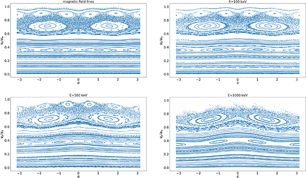
Figure 6. Poincaré sections of the magnetic field lines and of the particle trajectories in the  plane for the large amplitude case (3/2 and 5/2 mode amplitudes set to
  , 2/1 set to
  ) for energies 100 keV, 500 keV and 1 MeV.
Download figure:
Standard image High-resolution image104 electrons with an assigned energy and pitch angle distribution were initialized on different radial positions, uniformly distributed both poloidally and toroidally, and their orbits were followed for 104 toroidal turns. The particles are monoenergetic, with energy values chosen between 100 keV, 500 keV and 1 MeV, while the pitch angle was uniformly distributed in the ranges [−1, −0.7] and [0.7, 1]. The parameter p characterizing the order of fractional transport was calculated as the slope of the logarithm of  vs the logarithm of time, for each selected radial position. The same calculation can be performed by using
  versus time. An example of such curves for the large amplitude case and for the energy of the electrons 100 keV is displayed in figure 7. The curves in the large amplitude case tend to flatten for sufficiently large times because of electrons reaching the edge of the plasma and getting lost, so the calculation of the slope must be performed before this flattening takes place. The radial profile of p as calculated with the two different quantities is displayed in figures 8 and 9, over a radial range over which this quantity is sufficiently different from zero. The agreement in the values of p calculated with the two different methods is better in the large amplitude case than in the small amplitude case.
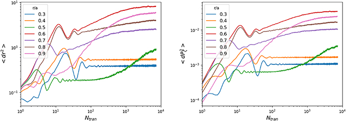
Figure 7.
 (left) and
  (right) vs
  , where
  is the number of toroidal transits, for the large amplitude case, for an electron energy of 100 keV.
Download figure:
Standard image High-resolution image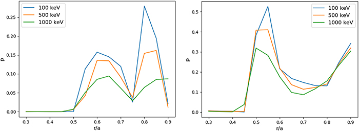
Figure 8. Level of subdiffusion p as calculated with  for the small (left) and large (right) amplitude cases.
Download figure:
Standard image High-resolution image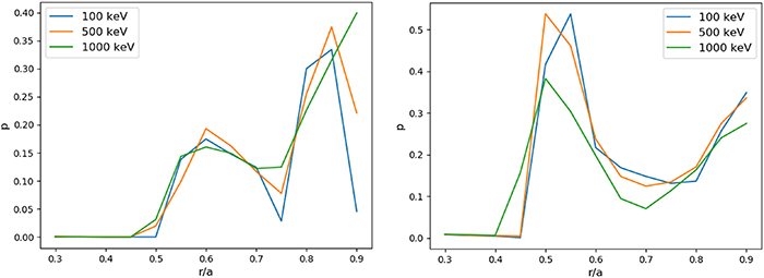
Figure 9. Level of subdiffusion p as calculated with  for the small (left) and large (right) amplitude cases.
Download figure:
Standard image High-resolution imageThe radial profile of the degree of magnetic stochasticity (Chirikov criterion [37]) and the structure of the perturbed magnetic surfaces (chains of magnetic islands) is displayed in figure 10 for the large and the small amplitude cases. The Chirikov parameter is computed locally, in the regions of space between two adjacent chains of magnetic islands, to quantify the radial variation of magnetic stochasticity. Values larger than one do not correspond to purely diffusive transport (p = 1) as the electrons do not spend sufficient time in these regions to enter diffusive regime. The drop in p ar  in the large amplitude case is attributed to trapping of particles in the large 2/1 magnetic island [5], while the increase at the edge of the plasma corresponds to large particle losses, because of complete breaking of magnetic surfaces. The purely diffusive regime with p = 1 is not reached under any of the circumstances we examined, which suggests that the level of magnetic perturbations is not sufficient to cause a complete stochastization of magnetic field lines under experimental conditions met during the flat-top phase of a RE discharge in COMPASS.

Figure 10. Chains of magnetic islands (left) and Chirikov parameter (right) for the large and the small amplitude cases.
Download figure:
Standard image High-resolution image6. Fractional diffusion
Fractional diffusion, unlike normal (or Gaussian) diffusion, does not present a universal behavior, and so it does not possess a characteristic time or length [27]. The non-existence of a characteristic time for fractional transport is related to its fractal character, that follows from the self-similarity of the structures leading to it. In the case of magnetic perturbations, this self-similarity occurs in the form of chains of magnetic islands. The curve describing the time dependence of the particle number has a rapid drop on the short times and then it decreases more slowly on the long time. The curve that best represents this behavior is the Mittag–Leffler function [38, 39], which interpolates between an exponential function and a polynomial. Mittag–Leffler functions are solutions of the fractional relaxation processes, and the solution comes in the form:
Examples of such functions are displayed in figure 11. An analytical solution of equation (1) can be attempted by separation of variables,  , and the time-dependent function T is in the form of a Mittag–Leffler function. However, the separation of variables works only if the diffusion coefficient Kp
is constant in time and the fractional exponent p is uniform in space. The analytical resolution procedure of equation (1) under these hypotheses is provided in the appendix
, and the time-dependent function T is in the form of a Mittag–Leffler function. However, the separation of variables works only if the diffusion coefficient Kp
is constant in time and the fractional exponent p is uniform in space. The analytical resolution procedure of equation (1) under these hypotheses is provided in the appendix

Figure 11. Mittag–Leffler functions with argument  for different values of p.
Download figure:
Standard image High-resolution imageThe fractional subdiffusive index p and the corresponding fractional diffusion coefficient Kp
, computed by using equation (3), can be used to numerically integrate the fractional diffusion equation. The level of subdiffusion p used in the numerical calculation and the fractional diffusion coefficient Kp
for the small and large amplitude cases are displayed in figures 12 and 13. The fractional diffusion equation equation (1) is solved by using a modified Crank–Nicolson algorithm [40], whose numerical implementation is described in the appendix

Figure 12. Level of subdiffusion p as calculated with  for the small (left) and the large (right) amplitude cases.
Download figure:
Standard image High-resolution image
Figure 13. Diffusion coefficient Kp for the small (left) and the large (right) amplitude cases.
Download figure:
Standard image High-resolution imageThe algorithm was tested against the analytical solution in the limit of uniform p and Kp
, and it was shown to behave correctly in the diffusive limit  . An initial runaway density distribution can be chosen and the fractional diffusion equation can be numerically solved. The relevant quantity for a comparison with experimental measurements of runaway losses is the particle number
  . The evolution of the density profile after 1 µs and the time evolution of the particle number for the large amplitude case is displayed in figure 14. for initial Gaussian and parabolic profiles. The Gaussian profile is centered on
  , where the 2/1 magnetic island is located; the parabolic profile is centered in the origin r = 0. N(t) show similar slopes for the same energies, regardless of the initial density distribution. The curves present the same character of the Mittag–Leffler functions, with an initial steep descent and a very gentle slope for long times, which follow an inverse-power law. In the examples here considered, the exponent of these inverse-power laws is below 0.1, which is smaller than the radial average of p. From the asymptotic expansion of the Mittag–Leffler functions, one would expect that
  , where p is some average value of p(t) over the radius, for sufficiently long times. Regardless of the exact value of this exponent, the calculation shows that the curves decrease, over sufficiently long times, with an inverse-power law with exponent smaller than one.

Figure 14. Density distribution n after 1 µs (left) and time evolution of the particle number N over 0.1 s (right) for an initial Gaussian and parabolic distribution (in black) of monoenergetic electrons.
Download figure:
Standard image High-resolution image7. Energy dependence
The usual assumption lying behind the use of the RR formula for the electron diffusion coefficient is that the particles follow closely the magnetic field lines. If we can reasonably neglect the finite Larmor radius (FLR) of the electrons, the same does not hold for the drift orbits, which must be taken into account correctly. The usual approach to this problem consists in introducing a correction factor resulting from a orbit-average procedure [41, 42]:
where  ,
,  is the drift-orbit radius, q is the safety factor and
  is the electron cyclotron frequency. λB
is the radial correlation length of the magnetic field fluctuations. x > 1 means that the transport is dominated by the perpendicular dynamics, while x < 1 means that the parallel dynamics is dominant. The correction factor Y expressed in equation (6) is always smaller than one and, for sufficiently large energies, it scales as the inverse of the particle energy, which means that the orbit average has the effect of suppressing RE transport. For the energies and the magnetic configurations we considered,
is the electron cyclotron frequency. λB
is the radial correlation length of the magnetic field fluctuations. x > 1 means that the transport is dominated by the perpendicular dynamics, while x < 1 means that the parallel dynamics is dominant. The correction factor Y expressed in equation (6) is always smaller than one and, for sufficiently large energies, it scales as the inverse of the particle energy, which means that the orbit average has the effect of suppressing RE transport. For the energies and the magnetic configurations we considered,  , which means that we would be always in the low-x limit of the curve. The drift-orbit radius of the electrons and the corresponding correction factor Y for the different energies is displayed in figure 15. The energy dependence is weak, because of the small values of
  and the relatively large λB
, which means that the drift-orbit average is little effective on suppressing the RE transport. The diffusion coefficient calculated according to the RR formula produces values that exceed the average value of the fractional diffusion coefficient Kp
by two–three orders of magnitude, so the orbit-average mechanism is not sufficient to justify the reduced RE transport.
and the relatively large λB
, which means that the drift-orbit average is little effective on suppressing the RE transport. The diffusion coefficient calculated according to the RR formula produces values that exceed the average value of the fractional diffusion coefficient Kp
by two–three orders of magnitude, so the orbit-average mechanism is not sufficient to justify the reduced RE transport.

Figure 15. Drift-orbit radius  (left) and energy-dependent correction factor Y (right).
Download figure:
Standard image High-resolution image8. Comparison with experiments
As explained in section 2, the correlation between RE losses and MHD activity can be observed by looking at the standard HXR signal and at the magnetic signals from Mirnov coils. Standard HXR can saturate if the radiation flux caused by the REs is too intense, which makes it unreliable for counting of losses. The signal obtained from shielded neutron detectors or photomultipliers located remote from the plasma can be used in its place, as they are mainly composed of HXR and they possess higher saturation thresholds. The presence of enhanced HXR and photo-neutron (peaks) in conjunction with the appearance of MHD modes, visible in the spectrograms, suggests that the RE losses follow a sudden increase, but after an initial burst the signal drops again, which might indicate a regime of subdiffusion. Fractional diffusion goes through an initially rapid phase, after which it enters a much slower phase which follows and inverse-power law for long times (see figure 14); the initial burst in the signal is thus attributed to the very initial phase of fractional transport. Such behavior can be observed in figure 16, where two such bursts in the photo-neutron signals can be observed at the onset of MHD activity, visible in the spectrogram as intense signals around 5–10 kHz, in shot #16 650.

Figure 16. Bursts of RE losses visible in photo-neutron signals at the onset of MHD activity, visible in the spectrogram as intense signals around 5–10 kHz, in shot #16 650.
Download figure:
Standard image High-resolution imageThe time integral of the HXR signal is assumed to be proportional to the RE losses; in typical RE experiments however the HXR fluxes span several orders of magnitude, so different detectors are used to cover this range [43]. By collecting the signals from detectors installed at different distances from the plasma and with different sensitivities, it is possible to cover a range of more than ten orders of magnitude. Signals from each detector must be selected in the range within which the detector exhibits a linear response; when the flux approaches the upper limit of this range, the signal tends to saturate. A chain of cross-calibrations between the signals of the different detectors can be performed when the signals display regions of partial overlapping. In the RE losses events that we considered here, only the less sensistive detectors (neutron detector and photomultiplier) were used to calculate the RE losses at the onset of the observed MHD activity; the HXR count rate properly calibrated and the corresponding time integrated signal are displayed in figure 17.
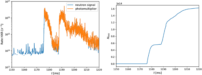
Figure 17. Calibrated HXR count rates (left) and time integrated signal (right) of shot #16 650.
Download figure:
Standard image High-resolution imageRE current is usually small in the flat-top phase of tokamak discharges but under particular conditions it can reach a significant fraction of the total current. In particular, this condition occurs when the plasma density is sufficiently low ( ) and the parallel electric field is much larger than the Connor–Hastie critical value (but smaller than the Dreicer value,
  ), which leads to a significant RE generation by Dreicer mechanism [44]. This have been observed in JET [45], Tore Supra [46], EAST [47] and COMPASS [48], where up to 50% of the total current was carried by REs. Similar plasma conditions were met in our case, which suggests that REs contribute to a significant fraction of the total current. The ratio
  and
and  during the flat-top of shot #16 650 is displayed in figure 18.
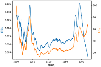
Figure 18.
 and
and  during the flat-top of shot #16 650.
Download figure:
Standard image High-resolution imageOhmic current was estimated by calculating electrical resistivity from the Spitzer formula. Density and temperature during the selected COMPASS discharge were obtained from Thomson scattering and interferometry data, while the parallel electric field was calculated from the loop voltage obtained from magnetic measurements. The radial density and temperature profiles reconstructed from Thomson scattering data are displayed in figure 19. The calculated plasma resistivity is on average 
 over the entire flat-top and the calculated ohmic current ranges from ∼20 kA to ∼100 kA against a plasma current deduced from magnetic measurements of 130 kA. The ohmic current has been calculated both with line-averaged density and temperature values, assuming a parabolic current profile, and with the volume integral of the current density, calculated with the reconstructed density and temperature profiles. The two results show good agreement. As a further evidence of a significant presence of REs, βN
measured by EFIT reconstruction was observed to increase during the flat-top phase, despite the fact that density and temperature remain approximately constant; βN
reaches values as high as 1.5, which is much larger than the value corresponding to plasma pressure alone. The comparison between βN
from EFIT reconstruction and calculated from plasma pressure is displayed in figure 20.
over the entire flat-top and the calculated ohmic current ranges from ∼20 kA to ∼100 kA against a plasma current deduced from magnetic measurements of 130 kA. The ohmic current has been calculated both with line-averaged density and temperature values, assuming a parabolic current profile, and with the volume integral of the current density, calculated with the reconstructed density and temperature profiles. The two results show good agreement. As a further evidence of a significant presence of REs, βN
measured by EFIT reconstruction was observed to increase during the flat-top phase, despite the fact that density and temperature remain approximately constant; βN
reaches values as high as 1.5, which is much larger than the value corresponding to plasma pressure alone. The comparison between βN
from EFIT reconstruction and calculated from plasma pressure is displayed in figure 20.
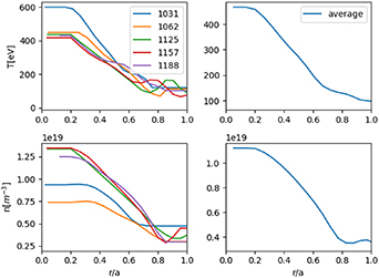
Figure 19. Density and temperature profiles reconstructed from Thomson scattering data for different instants during the flat-top (left) and their time average (right) for shot #16 650.
Download figure:
Standard image High-resolution image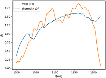
Figure 20. βN from EFIT reconstruction and calculated from plasma pressure (multiplied by 103) for shot #16 650.
Download figure:
Standard image High-resolution imageSpikes in the electric field develop whenever the total current drops; two main spikes develop in shot #16 650 at the beginning and at the end of the flat-top phase, when some MHD modes appear: this leads to some significant RE generation. Only the second spike is associated with significant RE losses, as the RE population at the beginning of the flat-top is very low. The time integral of the Dreicer generation rate, which is proportional to the RE density, displays well-defined steps, which qualitatively resemble those corresponding to the RE losses. The calculations return values in the order of several tens of kA, reaching up to 50% of the total current, compatible with the values reported in the literature and with the estimated ohmic component. The precise calculation is made difficult by the sensitive dependence of the growth rate formula for Dreicer generation on density, temperature and electric field, whose values are affected by experimental errors and fluctuations. To compensate for these fluctuations, which can be as large as 20% for density and temperature, a moving-average is performed over the signals. Within the variation range of these signals the calculated RE current can vary by on order of magnitude, producing values that are either exceedingly small or even larger than the plasma current. The evaluation of the ohmic fraction of the total current suggests that the calculation performed with the moving-averaged density and temperature values is representative of the actual RE current. We have not been able to reliably calculate RE generation in the early phase of the discharge as RE generation in the breakdown phase is more complicated and it cannot be described by Dreicer mechanism alone. The plasma current, parallel electric field, density and temperature during the flat top of shot #16 650 are displayed in figure 21, together with the Dreicer generation rate and the RE density.

Figure 21. Plasma current and parallel electric field (top left), density and temperature (bottom left), Dreicer generation rate (top right) and RE density (bottom right) during the flat-top of shot #16 650.
Download figure:
Standard image High-resolution imageThe time evolution of the RE number in the two events characterized by the spikes in the neutron signal is displayed in figure 22. The RE number at the beginning of the events has been normalized to one in order to show the relative drop and the curves have been time-shifted to make the initial instants coincide. An inverse-power law fit performed on the tail of these curves returns the exponents  and
and  for the first and the second peak respectively. The exact value of these exponents depends on the choice of the section of the curve over which the fit is performed; to analyze the behavior for long times, we performed the fit on the final part of these curves. These values are smaller than those calculated theoretically: the estimate of the RE losses from the HXR count is based on several assumptions, and the same goes for the calculation of the RE density evolution from the fractional diffusion model, so a quantitative comparison is still hard to reach. The qualitative agreement between the curves representing the RE losses in figures 14 and 22, however, suggests that the subdiffusive model we employed is correct.

Figure 22. Time evolution of the RE number following the losses in the two selected events in figures 16 and 17 in shot #16 650.
Download figure:
Standard image High-resolution image
9. Discussion
ORBIT simulations were performed to explore the character of RE transport in presence of small amplitude MHD perturbations ( –
– ) that take place in the flat-top phase of COMPASS discharges. The amplitude of the perturbations and the RE energies considered in this work are thus consistent with the ones observed in the experiments; in particular, the energies here considered correspond to small values of the electron Larmor radius (
 mm), which justifies the use of a guiding center code. Another reason for choosing a guiding-center code instead of a more computationally heavy full-orbit (FO) code is the need to perform a statistical analysis on the results, to evaluate the average square displacement of the particles from their initial position
  , which requires running simulations with thousands of particles over thousands of toroidal turns for many initial radial positions.
The subdiffusive character of particle transport observed under the considered conditions led us to model RE transport with a fractional diffusion equation, instead of resorting to the more largely used advection–diffusion model. This choice is motivated by the need to go beyond the currently used models, based on locality in space and time and on the random-phase approximation for the calculation of the diffusion coefficient. The fractional diffusion equation here adopted assumes that the fractional dependence of transport falls only on time: a more general space-time fractional diffusion equation would be more appropriate to describe this phenomenon. It is not possible to separately determine the spatial and temporal dependence of fractional transport with the method we have used here: to do so, a more fundamental approach based on the calculation of the probability distribution function and the waiting time distribution for the electrons must be followed.
The simulations performed with different electron energies show a suppression of RE transport as the energy is increased from 100 keV to 1 MeV. This results in smaller fractional exponent p, smaller diffusion coefficient Kp and smaller RE losses. This improved particle confinement for larger energies is usually attributed to a mitigating effect on the magnetic perturbations caused by drift-orbit average effects [41, 42] or by FO (FLR) effects [49]. FO effects were shown to mitigate transport of REs with energies of several MeVs and in presence of significant magnetic stochasticty. Here the FLR effects were neglected because of the small Larmor radius of the electrons, and the drift-orbit average effects calculated according to the theory developed by Hauff and Jenko, under the considered conditions, are non sufficient to account for the amount of suppression of RE transport which we observed.
The fractional diffusion equation was numerically solved for two initial RE density distributions, a parabolic one centered on r = 0 and a Gaussian one centered on  . This choice was motivated by the attempt to investigate how different initial distributions affect the evolution of the particle number. The results show that the time evolution of the density distribution and of the particle number is substantially independent of the initial distribution. This suggests that the density profile rapidly tends to a shape that depends only on the amplitude of the perturbation and on the electron energy, regardless of the initial distribution. The real RE distribution during the experiments is largely unknown, so a more realistic guess on the initial RE distribution could not be made, but the results suggest that the RE losses, according to the fractional diffusion model, do not depend significantly on this information.
The comparison with experimental measurements was performed on a couple of events where the onset of MHD activity during a discharge was accompanied by sudden RE losses, which could be observed as peaks in the photo-neutron signal. A cross-calibration between different HXR detectors makes it possible to estimate RE losses, while the calculation of the RE current during the flat-top phase of the discharge allows to evaluate the relative drop in the RE number. The power-law fit performed on the curves that describe the time evolution of the RE number during the loss events returns values that are compatible with subdiffusive transport. The procedure that has been implemented to achieve this result must be improved to make the quantitative comparison with theory possible.
10. Conclusions
The fractional character of RE transport in presence of MHD perturbations in COMPASS was addressed by performing particle simulations with the ORBIT code. The degree of subdiffusion p was deduced by calculating the average square displacement of the particles from their initial position  for different amplitudes of the perturbations and for different particle energies. The fractional diffusion coefficient Kp
was calculated by definition. The value of the fractional parameter p was always found to be smaller than one in the conditions we considered, which means that RE transport is subdiffusive. Time evolution of the RE number was calculated by numerically integrating a time-fractional diffusion equation, with p and Kp
deduced from the particle simulations. The long-time behavior of the particle number follows an inverse-power law with an exponent smaller than one, which is consistent with the asymptotic behavior of the Mittag–Leffler functions.
for different amplitudes of the perturbations and for different particle energies. The fractional diffusion coefficient Kp
was calculated by definition. The value of the fractional parameter p was always found to be smaller than one in the conditions we considered, which means that RE transport is subdiffusive. Time evolution of the RE number was calculated by numerically integrating a time-fractional diffusion equation, with p and Kp
deduced from the particle simulations. The long-time behavior of the particle number follows an inverse-power law with an exponent smaller than one, which is consistent with the asymptotic behavior of the Mittag–Leffler functions.
The energy-dependence of RE transport was assessed by performing simulations with different electron energies, ranging from 100 keV to 1 MeV: the result we observed is a suppression of RE transport as the energy is increased. The simulations we performed do not account for the FLR effects, which therefore cannot be invoked to justify this result. The drift-orbit average effects, predicted by Hauff and Jenko theory, have been calculated for the considered cases, but they are too small to account for our observations, which therefore must be explained by a different mechanism. The relativistic version of ORBIT correctly reproduces the drop of RE transport with the increase of the energy, but an intuitive interpretation of this behavior is still missing: in fact, the dependence of RE transport on the degree of magnetic stochasticity and on the RE energy reflects a complex dynamics which takes place in the 3D phase space of the system.
A comparison of the theoretical results with experimental measurements was performed by looking at the RE losses associated with MHD activity during a discharge. RE losses were estimated from neutron detector and photomultiplier, which have a higher saturation threshold than standard HXR. Time evolution of the RE number following these losses was calculated and an inverse-power law fit was performed on the tail of the corresponding curves. The fit returned exponents smaller than one, which is consistent with a fractional diffusion.
This study provides evidences that RE transport taking place in the flat-top phase of discharges in COMPASS, under the effect of small amplitude MHD perturbations, is subdiffusive. The qualitative confirmation of the fractional character of RE transport in experimental measurements supports this thesis. Suppression of RE transport as the electron energy is increased was observed in ORBIT simulations, but an intuitive explanation of this phenomenon is not available due to the complicated dependence of RE transport on the 3D phase space of the system. A simple formula providing the degree of fractional transport and the corresponding diffusion coefficient given the amplitude and spectrum of the perturbations and the RE energy does not exist yet, but a parametric study performed on a wide range of these values could fulfill the purpose. We were unable to separately determine the spatial and temporal dependence of fractional transport: a more advanced study based on a microscopic formulation in terms of continuous time random walks could overcome this limitation. We leave this task for a future work.
Subdiffusive transport of runaways is expected to take place whenever the magnetic configuration inside the plasma is not completely stochastic, which is the situation taking place when small MHD perturbations develop during the flat-top phase of a discharge. This might represent a serious issue for large devices, such as ITER, where a runaway seed can be generated and survive for a long time without being lost, eventually reaching high energies and causing serious damage to the plasma-facing components when it emerges to the plasma surface.
Acknowledgment
This work has been co-funded by MEYS Project LM2023045.
Appendix A:
If we assume that Kp
is uniform and constant, we can use Laplace transform ( ) in time:
where  is the Laplace transform of f, with
  . If
. If  , m = 1 and equation (7) becomes
  . We can separate then the time dependence from the space dependence and separate the variables:
  . In this way, the Laplace transform operates only on T, and we can divide both sides by R and
  :
:
Now the left-hand side only depends on r while the right-hand side depends on s. For equation (8) to make sense, both sides must be equal to a constant, that we can call  . In this way, equation (8) can be divided into a system of ordinary equations:
the first equation of equation (9) is the Bessel equation:  , whose solution is expressed in terms of zero-order Bessel functions:
  . The boundary condition in r = 0 imposes that
  , so that only the solution J0 survives. The solution for the space dependent part is expressed as an expansion in zero-order Bessel functions
  , where the eigenvalues λm
are the zeros of J0. The expansion coefficients are determined by the initial condition. The second equation of equation (9) can be inverted to find T. We assume for simplicity that
, where the eigenvalues λm
are the zeros of J0. The expansion coefficients are determined by the initial condition. The second equation of equation (9) can be inverted to find T. We assume for simplicity that  . The result can be written in the form of a Mittag–Leffler function [38, 39]:
The Mittag–Leffler function reduces to  for p = 1, which corresponds to the ordinary diffusion case. For
  ,
,  decays more slowly than an exponential, and tends to a constant for
  . When combining the results for the space and time components, the solution of the equation is:
Appendix B:
Using the following discretization for the fractional time derivative:
where  . The Crank–Nicolson algorithm with central difference implementation for the space derivatives leads to the following scheme:
where
 can be obtained by solving the linear system. The tridiagonal matrix of the coefficients makes the spatial part very easy to solve; the sum which is left on the right-hand side of the equation comes from the integral character of the fractional time derivative, and it represents the memory of the system.