


Abstract
One of the major challenges for the design of future thermonuclear reactors is the problem of power exhaust—the removal of heat fluxes deposited by plasma particles onto the plasma-facing components (PFCs) of the reactor wall. In order for the reactor to work efficiently, the power loading of the PFCs has to stay within their material limits. A substantial part of these heat fluxes can be deposited transiently during the impact of edge localised modes (ELMs), which typically accompany the high confinement mode, a regime foreseen for tokamak ITER and next-step devices. One of the possible ways to mitigate the deposition of localised heat fluxes during ELMs is injection of impurities, which could similarly to inter-ELM detachment dissipate part of the energy carried by plasma particles, the so-called ELM buffering effect. In this contribution, we report on experimental observations in impurity seeded discharges in ASDEX Upgrade, where injection of argon is capable of reducing the ELM energy by up to 80 (60
(60 without degradation of confinement). A simple model of ELM cooling is in some cases capable of providing quantitative prediction of this effect. The ELM peak energy fluence
  was reduced by a factor 8 without a degradation of the pedestal pressure. Should such mitigation be achieved in ITER, the resulting power loading would satisfy the material limits of divertor tungsten monoblocks (Eich et al 2017 Nucl. Mater. Energy12 84–90) and as such avoid the risk of their melting. The most favourable results in terms of confinement and divertor heat flux mitigation were achieved by use of a mixture of argon and nitrogen, where the later impurity helped to improve the confinement. The ELM frequency was identified as a scaling factor for
  in discharges with impurity seeding, suggesting that high frequency ELMs are favourable for future devices.
Export citation and abstract BibTeX RIS

Original content from this work may be used under the terms of the Creative Commons Attribution 4.0 license. Any further distribution of this work must maintain attribution to the author(s) and the title of the work, journal citation and DOI.
1. Introduction
The baseline scenario for burning plasma in ITER will be a high confinement mode (H-mode) [1] discharge with Type I edge localised modes (ELMs), as this regime offers the best performance in terms of Q. However, in presently-operated machines under attached conditions, this confinement mode is associated with large heat fluxes, which when scaled to the ITER device, represent a serious risk to the plasma-facing components (PFCs).
The heat fluxes during inter-ELM periods can be effectively mitigated in the regime of detachment with the aid of intensive fueling or impurity seeding [2]. However, the energy deposited during unmitigated Type I ELMs alone is expected to be sufficiently large to cause melting of the divertor tungsten monoblocks—the model for peak ELM energy fluence  developed by Eich [3] based on multi-machine experimental data set predicts target values between 9.4 (1:1 with respect to model) and 28 MJ m−2 (3:1 with respect to model), while threshold for melting of tungsten divertor is around 3 MJ m−2 [4, 5]. Therefore, a mitigation of
  by a factor of at least three (to 1/3:1 with respect to the model) is required to remain in safe operation. ELM mitigation and suppression techniques, such as magnetic perturbations [6] allow to adequately reduce the energy deposited by ELMs at the cost of reduced pedestal pressure [7, 8], which can compromise the ability to generate high fusion power.
One of the perspective tools for mitigation of ELM energy is the injection of impurities into the edge plasma. Similarly to inter-ELM detachment, the interaction between plasma and the impurity particles should transfer the thermal energy of plasma particles into radiation and as such avoid the deposition of highly localised heat fluxes at the divertor targets—this effect is dubbed ELM buffering [9]. However, previous attempts to achieve such a scenario at JET did not result in an appreciable reduction of deposited energy [9]. Moreover, fluid modelling of ITER ELMs in B2-Eirene suggests that significant ELM buffering is not feasible for large ELMs [10]. Experiments with impurity seeding at other tokamaks have sometimes resulted in a reduction of the ELM energy impacting at the divertor targets, however this was more likely achieved by a transition from Type I ELMy H-mode into a regime with smaller ELMs [11].
The objective of this work is to report on experimental observations at the ASDEX Upgrade, where significant ELM buffering (up to 80 of dissipated Type I ELM energy) and strong mitigation of the peak ELM energy fluence were observed in experiments with argon, neon and nitrogen seeding.
2. Scenario overview
The reference scenario for the experiments in the ASDEX Upgrade tokamak was a lower single null Type I ELMy H-mode with plasma current Ip
= 1.0 MA, toroidal magnetic field BT
= −2.5 T (ion  drift pointing towards the active x-point) and auxiliary heating
  = 10 MW,
  = 2 MW and
  = 1.9 MW. The plasma shape featured a relatively low triangularity (δl
= 0.4,
= 1.9 MW. The plasma shape featured a relatively low triangularity (δl
= 0.4,  0.18) with elongation κ = 1.7. Plasma fueling was typically kept constant (
 = 1.5 × 10²⁰ el s−1). A series of discharges was executed using either predefined waveforms or real-time feedback systems for the control of impurity injection. In the later case, the real-time measurement of power reaching the divertor
  [12] was used to control the injection of argon and a proxy measurement of electron temperature at the outer divertor target
  (using the divertor shunt currents [13]) [14] was used to regulate the injection of nitrogen. Figure 1 shows an example argon-seeded discharge
  38 320 with a pre-defined ramp on
  descending from 8 MW at t = 2.8 s to 4 MW at t = 5.6 s. It can be seen that the electron pedestal pressure pe
(using fixed ρ = 0.95) obtained by the integrated data analysis (IDA) diagnostics [15] remains constant at 7.6 kPa (corresponding to
descending from 8 MW at t = 2.8 s to 4 MW at t = 5.6 s. It can be seen that the electron pedestal pressure pe
(using fixed ρ = 0.95) obtained by the integrated data analysis (IDA) diagnostics [15] remains constant at 7.6 kPa (corresponding to  1) until t = 5.3 s.
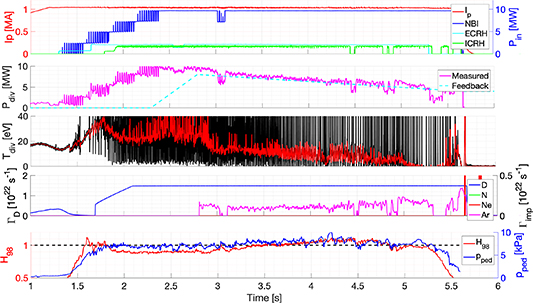
Figure 1. Overview of main plasma parameters of discharge  38 320 with argon seeding regulated by the real-time control system on
  .
.
Download figure:
Standard image High-resolution imageNote that  measurement is based on the assumption that the SOL current reaching the divertor plates is of thermoelectric origin, driven by the difference in electron temperature at the inner and outer targets. During detachment, this mechanism is significantly weakened (as the temperature is low on both targets) and other SOL current contributions (such as Pfirsch-Schlüter currents) may become dominant. In this case, the proxy can yield negative values and naturally ceases to be related to the electron temperature by means of a linear proportionality.
3. Divertor ELM impact analysis
3.1. ELM energy
The power dissipated during ELMs  was computed as the difference between (i) the energy released during the ELM
  and (ii) the energy deposited at the divertor target

While the former was derived from the changes of plasma stored energy  evaluated from a magnetic equilibrium reconstruction code during the course of each ELM, the later was obtained from the measurements of the infrared (IR) camera [16]. Since only IR measurements from the outer target were available, the power fraction flowing towards the outer target
  had to be determined:

Due to diagnostic limitations it was not possible to determine  directly. Instead, it was assumed that in the absence of extrinsic impurities
  =
=  (neglecting the role of intrinsic impurities and the power deposited onto first wall elements) and so the initial phases of discharges were used to determine
  (with typical values 0.6–0.7). Note that it is expected that the determination of the ELM energy using different diagnostics may be prone to systematic errors, which would propagate in this estimate of
  , therefore this quantity may not be a good representative of power sharing between the outer and inner divertor targets. It was also assumed that impurity injection does not influence the power sharing between the inner and outer divertor targets during the discharge.
Two methods of analysis of IR data were attempted. The first one used directly the measurements of surface temperature  and computed the energy required to achieve a given increase of
  during an ELM using a simple 1D model of heat conduction [17]:
where  is the fraction of tile surface exposed to plasma fluxes (equal to 0.8 for the AUG lower outer divertor) and cv
and κs
are heat volumetric capacity and heat conduction of tungsten respectively with weak dependence on temperature, which was approximated as:
is the fraction of tile surface exposed to plasma fluxes (equal to 0.8 for the AUG lower outer divertor) and cv
and κs
are heat volumetric capacity and heat conduction of tungsten respectively with weak dependence on temperature, which was approximated as:
Since the IR camera measures the entire poloidal profile of  the total ELM energy is calculated as a sum of energies corresponding to each pixel.
The duration of the ELM was determined by a combination of the measurements of IR and shunt currents. The shunt current measurements [13] were used to determine the ELM start and ELM end. However, in order to obtain  (which corresponds to the ELM rise time), the time evolution of peak surface temperature measured by the IR was used and
  was determined as a difference between time frame of minimum and subsequent maximum temperature within the ELM time window for each pixel separately (as shown in figure 2). The corresponding temperature difference for a given pixel is used as
  in equation (3).
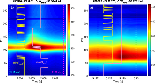
Figure 2. Measurements of  [∘C] during ELMs without seeding (a) and during argon seeding (b) in
  38 320. Yellow line indicates time frame with minimum temperature, pink line the time frame with a subsequent maximum of temperature. Blue and red dashed lines indicate the beginning and end of an ELM as measured by the shunt currents.
Download figure:
Standard image High-resolution imageThe second method of ELM energy determination is based on the output of THEODOR code [18], which converts the measurements of surface temperature into time evolution of impacting heat fluxes. The heat flux is then integrated along the target and for the duration of the ELM.
Both methods relied on the detection of ELM start and end times, which were based on measurements of shunt currents. Since these were also affected by impurity seeding, an adaptive threshold method was employed. The ELM was detected when the shunt current flowing in the outer divertor  exceeded a value of
  kA, where
  is the value of inter-ELM shunt current (obtained by rescaling of the
  signal as
 ![$I_\mathrm{inter-ELM} [A] = T_\mathrm{div}/0.02$](https://content.cld.iop.org/journals/0029-5515/63/12/126018/revision2/nfacf4aaieqn45.gif) ).
).
A comparison of the two methods for estimating the ELM energy is shown in figure 3(a). The agreement was satisfactory in most cases; however, during impurity seeding, in some cases the  yielded negative values, which were clearly unphysical due to volumetric radiation increasing the measured photon flux and leading to an overestimation of the surface temperature for some time slices [19]. This excess energy leads to an underestimation or even negative heat flux in consecutive time windows. In such cases
  provided larger values of ELM energy, representing a more conservative estimate of ELM buffering. This made
  a preferred quantity for further analysis.
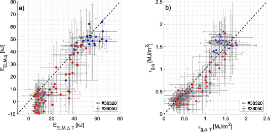
Figure 3. Comparison of ELM energy (a) and peak ELM energy fluence (b) deposited at the target by two different methods of IR analysis.
Download figure:
Standard image High-resolution image3.2. Peak ELM energy fluence
While the ELM energy is an important quantity for considerations of physics processes occurring in intra-ELM SOL plasmas, the magnitude of the peak ELM energy fluence  [3] is decisive for the interaction with divertor PFCs. Similarly to the calculation of the ELM energy,
  can be also obtained (i) using the increment of
  during ELMs or (ii) by integration of the heat flux obtained by the THEODOR code:
where  is the angle of impact of the magnetic field onto the divertor target (
 ). The agreement between these two methods is shown in figure 3(b). For consistency with ELM energy measurements,
  is used for further analysis.
In the following analysis, the ELM energy and energy fluence will be treated from different perspectives, however it is instructive to cross-check their correlations. As shown in figure 4(a), the values of  and
and  which are measured by IR at the outer target are reasonably well correlated. It would also be natural to expect that the measurements based on upstream or core measurements (
 and energy fluence model by Eich
  equation (8) in [3]) will exhibit a similar level of correlation, however this is clearly not the case, as shown in figure 4(b). One possible explanation for this poor correlation is that
  does not capture some hidden parameter. Indeed, previous experimental validations of this model have reported that most measurements are located between 1:1 and 3:1 multiples with respect to the model—apart from the original dataset used by Eich (which included data from AUG, JET and MAST), this behaviour was also confirmed at HL-2A [20], COMPASS [21] and to lesser degree in DIII-D [22]. Since the effect of buffering on ELM energy and fluence cannot be characterised jointly due to a weak correlation between
  and
and  , separate analysis for each of these quantities is presented in the following sections.
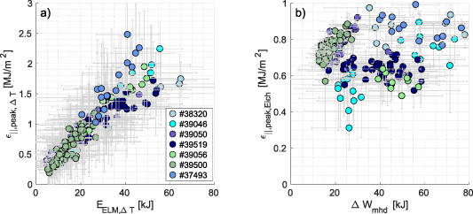
Figure 4. Correlations between ELM energy and fluence as measured at the outer target (a) and the ELM released energy measured by  and the predictions of peak ELM energy fluence using the Eich model (b).
Download figure:
Standard image High-resolution imageIn order to reduce scatter due to the individual differences between ELMs, data from 10 consecutive ELMs in a given discharge were combined, using the median for the representative value and standard deviation as an estimate of error.
3.3. ELM energy proxy
The divertor shunt current measurements  exhibited a convenient correlation with the ELM energy derived from the IR measurements (even during the impurity seeded phases of the studied discharges). This allowed for a construction of an ELM energy proxy
  , using the integral of this shunt current over the duration of the ELM (as shown in figure 5)
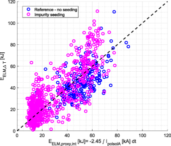
Figure 5. Comparison of ELM energy measured by the IR camera with a proxy based on shunt current measurements. Each point represents an individual ELM.
Download figure:
Standard image High-resolution imageThe correlation is not coincidental—the shunt current during ELMs occurs due to the thermoelectric effect [23], which is driven by the electron temperature difference between the inner and outer target. The ELM electron temperature is expected to be related to the ELM energy. This proxy allowed to obtain an estimate of ELM buffering even in discharges in which the IR camera did not yield useful data. This has the potential to be used in future real-time systems for the control of impacting ELM energy, similarly to the  control already used at ASDEX Upgrade. The correlation also indicates that the majority of ELM energy deposited at the outer divertor target is carried by charged particles and not by neutrals or photons.
4. Characterisation of ELM buffering
An example of ELM buffering measurement is shown in figure 6. In a reference discharge  39 487, where impurity seeding was not applied, the ELM energy measured at the outer target agrees with the energy released from the plasma (using
  0.8) and also with the energy estimated using an ELM energy proxy. An argon seeded discharge
  38 320 exhibits a large difference between
  and
and  at t
at t
 4.5 s, indicating significant energy dissipation of ELM energy, however the amount of impurity was not optimal, which caused an unintended increase of
  at t = 3.5–4.5 s and also eventually resulted in a disruption at t ∼ 5.5 s. Note that
  for highly buffered ELMs was ∼40 kJ, similar to the reference part of discharge prior to seeding, which indicates that also the ELM type was not affected by impurity injection. Finally, when both argon and nitrogen were injected in
  39 050, the discharge remained stable with good confinement.

Figure 6. Evolution of ELM energy in reference discharge without seeding  39 487 (a), argon seeded discharge
  38 320 (b) and discharge with combined argon and nitrogen seeding (c). ELM quantities are averaged over 10 consecutive ELMs.
Download figure:
Standard image High-resolution imageThe buffered fraction  defined as:
reached up to 80 in
in  38 320. However, at this point, the confinement and pedestal pressure were already degraded. Combined seeding in
  39 050 produced
  60
60 . Similar experiments were executed also with neon seeding, however these had to be accompanied by injection of nitrogen in order to maintain a stable discharge [24].
A comparative study using different impurities is summarised in figure 7. All discharges started with similar pre-seeding conditions and ELM frequency around 100 Hz. Despite numerous attempts, it was not possible to achieve significant ELM buffering ( 40
40 ) with nitrogen seeding only (figure 7(a)). However, injection of nitrogen typically leads to an increase in ELM frequency and reduction of ELM released energy (leading to the smallest ELM energies registered at the divertor target from all studied discharges). Pure argon seeding resulted in a decrease in ELM frequency and can produce large ELM buffering (up to 80
 ), however this was typically associated with a degradation of confinement (figure 7(b)). Combined nitrogen and argon seeding produces stable discharges with good confinement, high ELM frequency and significant ELM buffering (figure 7(c)). Finally, a combined neon and nitrogen seeding also resulted in significant ELM buffering. Unfortunately, there is only an indirect evidence of it (using ELM energy proxy, square symbols) since there were no useful IR measurements in any of the executed discharges with this impurity. Moreover, neon seems to have a long-lasting deteriorating effect on the plasma confinement, which escaped the simple characterisation used here (black outline for measurements with
  0.8 and magenta outline for
  0.8).
0.8).
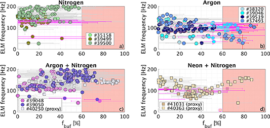
Figure 7. Dependence of buffered fraction on ELM frequency in case of nitrogen (a), argon (b), argon + nitrogen (c) and neon + nitrogen seeding (d). The red area indicates highly efficient ELM buffering. Square symbols represent measurements obtained using ELM energy proxy. Magenta outline indicates measurements with  0.8.
0.8.
Download figure:
Standard image High-resolution image5. ELM cooling model
A simplified model of ELM cooling is constructed in order to predict the magnitude of buffered energy. This model treats the ELM as an assembly of plasma particles having an initial Te
= Ti
equal to the pedestal electron temperature  . As such, the energy of the ELM is a sum of the energies of all its particles:
where  is the ion mean charge. The absolute number of ELM electrons
  can be determined at the point of ELM formation using the knowledge of the ELM released energy
  :
:
We assume that impurity cooling is the only loss channel of the ELM and we ignore the transport effects which may impact the cooling. All other interactions with the SOL plasma are also ignored (including the effect of the target sheath [25]) as well as energy transfer between ions and electrons, which was estimated by the free streaming model [26] to account for up to  of the electron energy (this magnitude of energy transfer was later confirmed experimentally at COMPASS [27] and measurements consistent with these predictions were also reported at JET [28]). In this greatly simplified picture the energy of the ELM changes as:

where  is the volume occupied by the ELM particles and
  is the cooling power due to the action of impurities in this volume. Using equation (10) and assuming the ion temperature remains constant, the change of ELM Te
can be expressed as:
is the cooling power due to the action of impurities in this volume. Using equation (10) and assuming the ion temperature remains constant, the change of ELM Te
can be expressed as:
Due to complex dependence of Lz
on Te
[29] this equation cannot be solved analytically but numerical solution can easily provide time evolution of Te
. Using the knowledge of the time  the ELM particles need to travel from upstream towards the target, the energy deposited at the target can be calculated as:

Subsequently, the buffered fraction can be expressed as:
The maximum buffered fraction predicted by this model ( ) is therefore equal to
  , ranging between 50
 (
( ) and 60
 (
( ). The predictions of this model using the divertor spectroscopy measurements [30] of argon and nitrogen impurity densities nAr
and nN
(assuming fixed
). The predictions of this model using the divertor spectroscopy measurements [30] of argon and nitrogen impurity densities nAr
and nN
(assuming fixed  = 1.1 in absence of direct measurements of this quantity) are shown in figure 8. In discharges
  38 320,
  39 046,
  39 056 the model has good quantitative agreement with the experiment, which is a splendid result, given the fact that the model has no tuning parameters and is therefore fully predictive. However, in other discharges, the model underestimates the amount of buffering by up to factor 50. There are a number of reasons why this could occur, most probably because the location of the impurity concentration measurements is not representative of the impurity concentration used in the model or the omission of ELM interaction with neutrals. The model is non-linearly sensitive to impurity concentration, as demonstrated in figure 9(a), where the ELM cooling model was calculated for a selected ELM in
  38 320 using the measured value of nAr
as well as its 0.5 and 1.5 multiple (indicating the uncertainty of the measurement). This is a result of the strongly varying magnitude of Lz
with Te
(see figure 9(b)): as soon as ELM Te
cools down to ∼300 eV, the subsequent cooling is greatly accelerated and in some cases the Te
is reduced practically to zero. Unfortunately, this strong dependence is interfering with the actual precision of the impurity concentration measurements, which was estimated to be 50
38 320 using the measured value of nAr
as well as its 0.5 and 1.5 multiple (indicating the uncertainty of the measurement). This is a result of the strongly varying magnitude of Lz
with Te
(see figure 9(b)): as soon as ELM Te
cools down to ∼300 eV, the subsequent cooling is greatly accelerated and in some cases the Te
is reduced practically to zero. Unfortunately, this strong dependence is interfering with the actual precision of the impurity concentration measurements, which was estimated to be 50 .
.

Figure 8. Comparison of the heuristic model for ELM buffering with experimental observations.
Download figure:
Standard image High-resolution image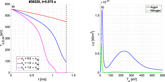
Figure 9. Time evolution of ELM electron temperature with varying impurity density (a), the temperature dependence of the cooling factor Lz (b). The values of Lz were obtained from [29].
Download figure:
Standard image High-resolution imageHowever, there are probably other factors influencing the magnitude of buffering, as suggested by a comparison of similar discharges  38 320 and
  37 493 (both argon seeded). While the argon density and concentration were systematically lower in
  37 493 (see figures 10(a) and (b), the buffered energy devised from IR measurements was actually higher even though the initial ELM energies were similar in both discharges, as shown in figure 10(b). At the time of writing, these factors have not yet been identified.
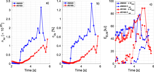
Figure 10. Argon densities (a), concentrations (b) and ELM buffering (c) in discharges  38 320 and
  37 493.
Download figure:
Standard image High-resolution image6. Peak ELM energy fluence
The peak ELM energy fluence  was compared to a model developed by Eich et al [3] (see figure 11)
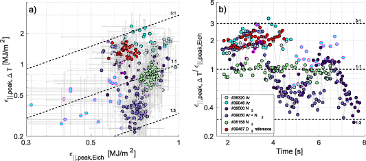
Figure 11. Measurements of peak ELM energy fluence  compared to the predictions of ELM model [3] (a) and the evolution of the normalised fluence in time for selected discharges (b).
Download figure:
Standard image High-resolution imagewhere a is the plasma minor radius, κ plasma elongation,  a geometrical factor (assuming ∼2.0 for AUG) and
  = 4.2 is the ratio of toroidal and poloidal magnetic fields in the outer midplane. The reference discharge
  39 487 and the measurements prior to seeding in other discharges are located between 1:1 and 3:1 line, similarly to previously reported measurements at AUG. It can be seen that impurity seeding leads to a significant reduction of
  , eventually reaching the 1:3 line. At this level, their impact is comparable to the I-mode pedestal relaxation events [31]. The trajectory of such discharges in figure 11(a) is almost vertical, so unlike other ELM mitigation techniques, impurity seeding evades Eich's model. In case of discharges with confinement degradation (such as
  39 046) the discharge trajectory is better correlated with the predictions of the model.
The ratio  can be reasonably well parametrised using the ELM frequency
  , as shown in figure 12(b). In these discharges, where the injection of impurities resulted in an increase of
  , the changes in peak ELM energy fluence can be characterised by the following model:

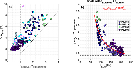
Figure 12. Comparison of the peak ELM energy fluence and the ELM size (a) and the dependence of the peak ELM energy fluence on ELM frequency (b).
Download figure:
Standard image High-resolution imageThis scaling describes the evolution of  within the boundaries of validity of the Eich model (between 1:1 and 3:1 lines) but also measurements below the 1:1 line. It is natural to suspect that
  is not the real driving parameter but perhaps a proxy which is correlated with other undetected parameters with some link to the concentration of impurities and neutrals. However, at the time of writing these parameters have not been resolved. On the other hand,
  is a convenient parameter for practical purposes, with a potential for implementation in real-time control systems.
It can be seen that the variation of  is significantly larger (factor 8 in
  39 056) than that of
  , which may be surprising since the energy and peak ELM energy fluence of the ELMs are tightly correlated (as demonstrated in figure 4(a)). As mentioned earlier, the additional dynamic range of
  stems from the precision of Eich's model—as reported by Eich the experimental values even without any effect of impurities vary between 1:1 and 3:1 line.
As demonstrated in figure 12(a), the largest reduction of  is achieved for ELMs of small size (
 2
2 ), which is consistent with the favourable scaling with
  .
.
Note that the Eich model presented in equation (16) was verified only for Type I ELMs. While the ELMs in prior to the beginning of the seeding are clear Type I ELMs, it is in practice impossible to verify the nature of the buffered ELMs due to the dynamic evolution of the discharges. However, since significant reduction of  can be achieved without confinement degradation, it is still assumed that these buffered ELMs are relevant to ITER.
7. ELM buffering relation to detachment and plasma confinement
The use of impurities to dissipate power in the SOL draws its inspiration from the physics of detachment, which is relevant to inter-ELM plasma conditions. However, a comparison of the ELM buffering fraction with the proxy for inter-ELM temperature  (see figure 13) shows a complex relationship between the impact of impurities in intra- and inter-ELM plasma conditions.

Figure 13. Divertor temperature proxy  versus the buffered fraction. Magenta outline indicates degraded confinement (H98(y,2)
  0.8).
0.8).
Download figure:
Standard image High-resolution imageThe reference discharge  39 487 is clearly attached, with
  30 eV. In case of argon-seeded discharges there is a notable drop in
  to ∼5 eV even when
  is small. For high
  there is a clear anti-correlation between the two quantities, meaning that with high
  the discharge approaches partial detachment. However, reaching
  0 eV was only possible at the cost of a degraded confinement.
In the case of nitrogen-only seeding, the  and
and  appear to be de-correlated—the discharge
  35 158 reaches negative
  (which is considered as an indication of partial detachment) without a significant ELM buffering. This suggests that a mixture of different impurities may be required to achieve simultaneously inter-ELM detachment (using light impurities) and ELM buffering (using heavier impurities). This strategy is consistent with the idea of significantly different electron temperatures being relevant in the two phases of the ELMy H-mode.
When considering the suitability of impurity seeding for future thermonuclear reactors, it is essential to assess the effect of injected impurities on the confinement, here represented by the H-factor H98(y,2). The relation between the buffered fraction and the quality of confinement is shown in figure 14(a). The pre-seeded phases of discharges and the reference discharge  39 487 are characterised by H98(y,2) = 0.9.

Figure 14. Confinement quality expressed using  versus the buffered fraction
  (a) and relation between
  and the buffered fraction (b).
Download figure:
Standard image High-resolution image
Argon seeding was initially allowed to reach H98(y,2) = 1. However, then confinement typically deteriorated to H98(y,2) ∼ 0.8 for high buffered fractions. Nitrogen seeding was not capable of producing strong buffering, however it helped to improve the H-factor up to 1.1 (this behaviour has already been reported at ASDEX Upgrade [32]). The optimal results were achieved by a combination of argon and nitrogen seeding with high buffered fraction (∼60 ) and reasonable H-factor of 0.95 (discharge
  39 050). Obtaining higher buffering fractions (
 60
60 ) was always only intermittent and typically already followed by a strong degradation of confinement or even a disruption. This appears to be consistent with the simple model for the limit of ELM buffering presented in section 5—
 above
above  would require a reduction of ion temperature during the ELM transport in the SOL. Figure 14(b) shows clearly that increased
  always correlated with an increase of
  .
.
8. Conclusions and outlook
Experiments with argon, neon and nitrogen seeding were used to investigate the ELM buffering phenomena at AUG. It was observed that argon is necessary to achieve significant buffering fraction  40
40 , however argon-only seeded discharges suffered from degradation of confinement to
  0.8. This shortcoming was resolved by the addition of nitrogen, which on its own was unable to produce significant ELM buffering, however it had a positive role in the confinement of the discharge and also aids in achieving inter-ELM detachment.
A simplified model of ELM cooling using divertor impurity concentration measurements was proposed for the prediction of the magnitude of buffered ELM energy. While some discharges with argon-only seeding seem to be in a reasonable agreement with the model, there is still a large room for its improvements. The model predicts the maximum buffering to be between 50%–60 depending on the
  .
.
The studied discharges were in agreement with Eich's model for the peak ELM energy fluence, except for the case of strong buffering, where the measured  was up to three times lower than the prediction of the model. These results suggest that mitigation of divertor heat loading by a mix of radiative impurities may help to alleviate the potential component damage caused by edge transients. The reduction of
  is large enough to become marginally acceptable for ITER from the point of view of PFC melting risk. Since the buffering is not expected to change the ion energy, there can still be detrimental consequences for PFCs due to increased material erosion during ELMs.
As a next step, the process of ELM buffering will be studied using the 1D3V particle-in-cell code BIT1, which is capable of simulating the temporal evolution of an ELM as well as different collisional processes in the SOL. The modelling will help to improve the simplified model presented in this work.
In future experiments, it would be desirable to develop a real-time control system, which would regulate the impurity seeding rate in order to maintain a desired impacting ELM energy. The ELM energy proxy based on divertor shunt current measurements represents an example of a sensor which could be implemented in such a system.
Acknowledgments
Authors would like to thank Thomas Eich for valuable discussions on the model for peak ELM energy fluence and Thomas Pütterich for kindly providing data on the cooling factors. This work has been carried out within the framework of the EUROfusion Consortium, funded by the European Union via the Euratom Research and Training Programme (Grant Agreement No. 101052200 - EUROfusion). Views and opinions expressed are however those of the author(s) only and do not necessarily reflect those of the European Union or the European Commission. Neither the European Union nor the European Commission can be held responsible for them. This work has been supported by MYES Project CZ.02.1.01/0.0/0.0/16 013/0001551 and Czech Science Foundation Project GA20-28161S.