


Abstract
Reliable modeling of macroscopic melt motion induced by fast transients requires the accurate and computationally efficient description of the emitted current density that escapes to the pre-sheath. The ITER sheaths that surround hot tungsten surfaces during edge-localized modes are characterized by important contributions from secondary electron emission and electron backscattering as well as by the coupling between thermionic emission and field electron emission. Under the guidance of systematic particle-in-cell simulations that incorporate a comprehensive analytical electron emission model, a highly accurate semi-empirical treatment of the escaping electron current has been achieved.
Export citation and abstract BibTeX RIS

Original content from this work may be used under the terms of the Creative Commons Attribution 4.0 license. Any further distribution of this work must maintain attribution to the author(s) and the title of the work, journal citation and DOI.
1. Introduction
The narrow interface between plasma-facing components (PFCs) and standard scrape-off-layer plasmas can be accurately described by the classical model of quasi one-dimensional ion sheaths [1–5]. Regardless of the magnetic field line inclination with respect to the local surface normal, the plasma region closest to the material boundary is the non-neutral Debye sheath; an ion-rich strongly inhomogeneous region where the electrostatic field points from the plasma to the boundary with monotonically increasing magnitude. Various conditions need to be satisfied for the standard description to be applicable such as negligible cross-field drifts, low plasma collisionality, perfect boundary planarity and weak electron emission [6].
Considerable attention has been recently paid to the violation of the weak electron emission condition owing to intense thermionic emission (TE) from hot tungsten (W) divertor plates [7]. This is of particular significance for ITER, as it is tightly connected with gross topological damage due to macroscopic W melt motion induced by fast transient events such as edge localized modes (ELMs) [8, 9]. More specifically, as a consequence of the localized ELM-wetted area, the incident plasma fluxes can be assumed to remain nearly ambipolar. Thus, a non-ambipolar current density arises that is equal to the thermionic current density which escapes to the Bohm pre-sheath. The bulk replacement current density generated by this escaping current is responsible for a strong volumetric Lorentz force that drives metallic melt motion leading to macroscopic erosion [10]. Dedicated misaligned exposures in JET [11], ASDEX-Upgrade [12], WEST [13] and modeling with the MEMOS-U code [14–16] have confirmed this picture.
In contemporary metallic tokamaks, the weak electron emission condition can be violated in the divertor during intra- and even inter-ELM periods. At very elevated surface temperatures, the nominal emitted current density owing to TE, as described by the Richardson–Dushman formula [17], is so intense that it becomes incompatible with the classical Bohm pre-sheath structure. As a consequence, space charge accumulation in the sheath leads to the formation of a virtual cathode (VC) that limits the escaping thermionic current to a constant value, since the reversal of the electrostatic field direction causes the recapture of a fraction of the emitted thermo-electrons. Thus, there is a transition from a monotonic to a non-monotonic potential profile, with the latter known as the space-charge limited (SCL) regime of the emissive sheath [18, 19]. In the case of oblique magnetic field inclination angles, the SCL transition is still realized [20], but further complications arise due to the suppression of the nominal thermionic current by recapture during Larmor gyration [21, 22]. In present-day tokamaks, the SCL transition generally occurs at surface temperatures below the W melting point, which implies that SCL sheaths nearly exclusively surround molten W PFCs. The SCL regime of thermionic emissive sheaths has been thoroughly studied in our previous works, where an accurate semi-empirical analytical expression for the limited value of the escaping thermionic current as a function of the plasma conditions and magnetic field inclination angle was constructed on the basis of particle-in-cell (PIC) simulations [7, 20, 23].
On the other hand, during ITER intra-ELM periods, the predicted high electron temperature and plasma density in the pre-sheath edge should have strong impact on the emissive sheath established above the hot W PFCs. In particular, it has been demonstrated that the elevated electron plasma temperatures enable significant contributions from electron-induced electron emission (secondary electron emission (SEE) & electron backscattering (EBS)) [EIEE], that the intense normal wall electrostatic fields lead to strong coupling of TE with field electron emission (primarily in the Schottky regime) and that the intense incident plasma particle fluxes push VC formation at much higher surface temperatures, so that the monotonic potential profile regime becomes relevant for W melt motion [24]. To facilitate the exploration of this novel multi-emissive sheath regime, a comprehensive W electron emission model was recently implemented in the 2D3V SPICE2 PIC code that features accurate state-of-the-art analytical descriptions for the yields, the energy distributions and the angular distributions for the processes of field-assisted TE, SEE and EBS [24].
Modern three-dimensional computational models of metallic melt events require the evaluation of the escaping current density at each time step and each grid point of the PFC free surface. Therefore, it is crucial that the description of the current density that escapes from the multi-emissive Debye sheath to the Bohm pre-sheath is as simple and computationally efficient as possible without compromising the accuracy. Here, we address the ITER-relevant multi-emissive sheath at normal magnetic field inclination; relevant to the worst-case scenario of exposed leading edges that may occur due to tolerance build-up during PFC manufacturing and installation [8, 9]. Highly accurate simple analytical semi-empirical expressions are provided for the SEE, the EBS and the field-assisted thermionic current densities in the monotonic potential regime as well as for the total escaping current density in the SCL regime. The semi-empirical expressions have been guided by and benchmarked against comprehensive 2D3V SPICE2 PIC simulations. The expressions can be directly introduced in melt dynamics codes as the only non-trivial boundary condition of the boundary value problem for the replacement current density that propagates in the melt layer.
2. Electron emission model
The electron emission model for field-assisted TE, SEE and EBS from pure W has been described in [24]. In what follows, we summarize the main expressions to keep the manuscript self-contained.
The analytical treatment of field-assisted TE within the so-called extended Schottky regime is based on the established current density formula [25, 26]
where  is the surface temperature,
  is the normal electrostatic field strength at the wall,
  eV is the work function of polycrystalline W at room temperature [27–29],
  [28–30] is the effective Richardson constant of W,
  (in cgs units),
  is the reduced Planck constant,
  the electron mass, e the elementary charge and
  the Boltzmann constant. The standard Schottky regime naturally emerges when
  [25], which leads to
where  stands for the Schottky correction to the material work-function [31], with
  leading to the Richardson–Dushmann formula [17, 31]
The velocity distribution of thermionic electrons follows a half-Maxwellian distribution of temperature  [17, 31].
The analytical treatment of the SEE W yield is based on the Young–Dekker formula for the normal yield with optimized range energy exponents based on the Walker et al experiments [32–34] combined with a power secant law for the oblique yield which strongly saturates at near-grazing incidence and features an optimized energy dependent exponent  based on the Bronshtein–Fraiman experiments [35]. It reads as

where  is the incident electron energy, θ the incident electron angle with respect to the surface normal,
  ,
,  eV, k = 1.38,
  ,
,  and
and  . The energy and angular distributions of the secondary electrons follow the Chung–Everhart [36] and Lambertian [37] distributions
with E the exit kinetic energy,  the solid angle and Θ the exit angle with respect to the surface normal.
The analytical treatment of the EBS W yield is based on the empirical half-sigmoid description for the normal yield [38] with optimized coefficients based on the El Gomati et al experiments [39] combined with the general observation that the yield logarithm is a linear  function [40, 41] and assuming an empirical half-sigmoid form for the asymptotically tangential incidence yield with optimized coefficients based on the Bronshtein–Fraiman [35] and Neubert–Rogaschewski experiments [42]. It reads as


where  ,
,  ,
,  ,
,  ,
,  and
and  . The energy distribution of backscattered electrons follows the Jablonski–McAfee distribution [43, 44], while the angular distribution assumes
  diffusive Lambert contribution and
  specular reflective contribution [45]
where  is the reduced exit kinetic energy and
  is the Everhart coefficient for W.
3. Problem formulation
The problem comprises the calculation of the total emitted electron current density that escapes from the electrostatic Debye sheaths of multi-emissive character, which surround hot biased W PFCs during ITER ELM periods, to the classical Bohm pre-sheaths. In view of macroscopic melt motion applications, the main objective concerns the formulation of an accurate and computationally efficient analytical treatment of the escaping current density. Thus, a number of assumptions are necessary in order to simplify the problem prior to its numerical implementation in the 2D3V SPICE2 PIC code [7, 20, 23, 24].
The assumptions below are followed in all simulations: (a) Irrespective of the emission strength, the wall is biased with respect to the quasi-neutral plasma with a  magnitude that is determined by the ambipolarity of the incident plasma fluxes. The fixed bias stems from the fact that the W PFC is electrically connected to the grounded vessel and from the assumption that the localized emissive sheath is unable to affect the global plasma potential. (b) Irrespective of the emission strength, the classical Bohm pre-sheath potential structure is unaltered by the escaping emitted electron current. In particular, the ions are injected at the plasma boundary with a parallel to the magnetic field speed distribution satisfying the Bohm criterion [46]. As a consequence, there is no possibility for an inverse sheath formation [47–49]. (c) All the charged species are collisionless. This is well justified for both the plasma species during intra-ELM periods, but might be violated for the cold emitted electron populations. (d) The effects of the plasma neutrals stemming from surface neutralization or from three-body recombination are assumed to be negligible given the high plasma temperatures of interest. The effects of impurity neutrals stemming from material vaporization are also assumed to be negligible given the surface temperatures of interest. Only at extremely elevated surface temperatures, when vaporization is significant and vapor shielding effects are dominant, neutral generation and dynamics should also be included [50]. (e) The material boundary is perfectly planar. Debye-scale surface roughness could potentially affect EIEE by altering the average plasma electron impact angle, affect field-assisted TE by modifying the normal wall electrostatic field and even seed potential non-uniformities in the presence of VCs [51]. (f) The plasma and material boundary conditions are homogeneous. The simulations assume a homogeneous quasi-neutral plasma boundary and an infinite emitting surface boundary with a homogeneous prescribed temperature [7, 24].
Since the objective is the development of a general simple analytical treatment of the multi-emissive sheath, the assumed plasma parameters are not critical, but should still be representative of the ITER intra-ELM period [24]. ITER will need to achieve high levels of ELM suppression with resonant magnetic perturbation fields, pellet pacing and alternative techniques [52]. ELM mitigation mainly concerns the transient heat pulse magnitude on shaped divertor monoblocks in the high heat flux areas of the vertical targets. While substantial experimental effort will be made to develop effective ELM control during the earlier phases of ITER operation, it is inevitable that some unmitigated or partially mitigated ELMs will occur at high performance [9]. These rare cases are the primary target of ELM-induced melt motion studies, whose objective is to scope the heat flux thresholds and allowed ELM numbers before damage occurs at an extend that may threaten long-term power handling capabilities. Hence, such cases should also be targeted in our investigation. An established multi-machine scaling for the peak parallel ELM energy fluence
 , that is based on measurements in ASDEX Upgrade, JET and MAST [53], leads to the ELM energy densities of
  MJ m−2 for the ITER baseline scenario, for which
  MA,
MA,  T [9]. In accordance with a recent systematic investigation of the ITER W monoblock surface melting and toroidal gap melting limits [54], we shall consider partially mitigated
  MJ m−2 ELMs that are deposited as square heat flux pulses of
  GW m−2 at the outer vertical target (OVT) and of
  GW m−2 at the inner vertical target (IVT) over a duration which corresponds to the
  s expected ELM decay time [24]. Given the predicted
  keV pedestal temperature for the ITER baseline scenario [55], kinetic simulations of large JET ELMs [56] and conflicting experimental results [57, 58] as well as the strong spatiotemporal temperature variations during ELMs, the choice of
  eV was deemed as reasonable. Finally, the knowledge of
  ,
,  allows the calculation of the electron density at the sheath entrance from
  , where γ denotes the sheath heat transmission coefficient,
  denotes the sound speed and α is the magnetic field line inclination angle with respect to the surface tangent plane. Utilizing the standard high
  value of the sheath heat transmission coefficient (γ = 7) [3], assuming an isothermal plasma (
 ), employing
  for the average ion mass in deuterium–tritium mixtures and substituting for
  (3.7∘) for the OVT (IVT) inclination angle, one ultimately acquires
  m−3 for the OVT,
  m−3 for the IVT. Note that the magnetic field strengths corresponding to
  T are
T are  T for the OVT,
  T for the IVT. It should be strongly emphasized that, although the above grazing inclination angles have been employed for the prescription of the plasma parameters, we shall exclusively focus on the case of normal inclination angles, i.e. on
  , that corresponds to exposed OVT and IVT leading edges.
4. PIC simulations
Sheath Particle-In-Cell (SPICE2) is a 2D in space and 3D in velocity (2D3V) Cartesian PIC code that calculates the motion of charged particles within a prescribed static magnetic field and their self-consistent electrostatic field. The SPICE2 code has been optimized for the collisionless simulations of the electrostatic sheaths and magnetic pre-sheaths of PFCs oriented at oblique angles with respect to the magnetic field lines [59–61]. In all our simulations, ions are assigned a unique  mass to approximately account for the 50/50 deuterium—tritium burning plasma fuel mixture. Details of the implementation of field-assisted TE and of EIEE have been reported elsewhere [7, 23, 24]. In what follows, we shall present the overall simulations performed and focus on some numerical peculiarities that are associated with the implementation of the Schottky effect in the vicinity of the transition to the SCL regime.
Systematic IVT-focused, OVT-focused and parametric PIC simulations have been performed aiming to construct and to validate the semi-empirical analytical treatment. In the parametric simulations, the electron temperature has been widely varied for constant plasma density given the large respective uncertainty during ITER intra-ELM periods and especially partially mitigated ITER ELMs [52]. The simulations can be categorized in five batches: (a) PIC simulations that only consider EIEE (SEE and EBS). About 16 such simulations have been carried out for  m−3 varying the electron temperature within 500–2000 eV in steps of 100 eV. (b) PIC simulations that only consider TE without complications due to the Schottky effect. About 20 such simulations have been performed for IVT and OVT conditions by varying the surface temperature within 3600–5400 K in steps of 200 K. (c) PIC simulations that only consider TE including the Schottky effect. About 31 such simulations have been carried out for IVT and OVT plasma conditions by varying the surface temperature within 3400–5000 K in steps either of 100 K or of 200 K. (d) PIC simulations that consider TE without complications due to the Schottky effect together with EIEE. About 19 such simulations have been performed by varying the surface temperature within 3600–5200 K (IVT conditions) or 3600–5400 K(OVT conditions) in steps of 200 K. (e) PIC simulations that consider TE including the Schottky effect together with EIEE. About 16 such simulations have been performed for IVT and OVT conditions by varying the surface temperature within 3600–5000 K in steps of 200 K.
The basic post-processed output of these 102 PIC simulations consists of the incident plasma current densities, the emitted electron current densities and their standard deviation, the normal wall electrostatic field, the average plasma electron incident energy, the average plasma electron incident angle w.r.t. the wall normal and the VC depth. These PIC data are available online [62].
The simulation setup is designed in a manner very similar to [24]. However, for the purposes of this investigation, the implementation of the Schottky correction  to the work function
  had to be updated. The SPICE2 code self-consistently calculates the normal electrostatic field strength at the wall in order to determine the magnitude of the Schottky correction
  (in cgs). The effective work function,
  , strongly influences the magnitude of the escaping electron current density, see equation (1) or (2), which in turn affects the entire profile of the sheath electrostatic field. This feedback loop problem has been resolved by a simple iterative procedure where; starting from the material
  , i.e. essentially the Richardson–Dushman equation (3) formula, the
  value is updated in a step-wise manner after every few thousand temporal iterations, based on the current magnitude of the normal wall electrostatic field. In most cases, this algorithm yields satisfactory results. However, for parameters in the vicinity of the transition to the SCL regime, it generates strong oscillations in the escaping current density. This is caused by the fact that, for such parameters, the unimpeded thermionic current density (with the material
  ) is not intense enough for a VC to form. Nevertheless, when the Schottky correction is applied, then the escaping current density is increased so that the VC now emerges. This implies a change in the wall electrostatic field sign, which naturally disables the Schottky correction in the next iteration of the simple algorithm. While these oscillations cannot be completely suppressed, it was found possible to mitigate them efficiently by introducing a damping term β in the calculation of the effective work function
  :
:

where β = 1 corresponds to no damping introduction and β = 0 to no update of the effective work function. The algorithm performance with β = 1 and β = 0.2 is depicted in figure 1. The latter leads to satisfactory precision without significantly extending the simulation duration.
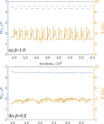
Figure 1. Numerical instability in the work function and total current density near the SCL transition. PIC simulations (TE + SEE + EBS) for OVT conditions at  K. (a) Large oscillations for β = 1.0. (b) Weaker oscillations for β = 0.2.
Download figure:
Standard image High-resolution image5. Results
5.1. Semi-empirical description of the EIEE yields
In case of a constant sheath potential drop  , the realization of TE at high surface temperatures does not affect EIEE (SEE & EBS) even within the SCL regime. This is a direct consequence of the vastly different energy distributions of the emitted electrons. VC formation naturally counteracts the propagation of the most populous emitted species (TE) and thus has a depth that is of the order of
  . Therefore, VC formation cannot affect the dynamics neither of the 10 × more energetic secondary electrons nor of the 1000 × more energetic backscattered electrons. As a result, in order to extract an analytical description of the effective EIEE yields, it is more convenient to perform PIC simulations with SEE & EBS, in absence of TE.
PIC simulations have been performed for varying electron temperatures in the absence of TE and the average SEE (EBS) yields have been extracted from the ratio of the emitted SEE (EBS) current over the incident electron current. In particular, 16 SPICE2 2D3V simulations have been carried out with  500–2000 eV (varying in steps of 100 eV) and
  m−3.
m−3.
As in all standard one-dimensional sheath models, the theoretical effective EIEE yields have been computed by a weighted velocity average of the EIEE particle flux over the Maxwellian velocity distribution [63],
where the perfectly planar wall has been assumed to be oriented parallel to the yx plane so that vz
denotes the normal velocity component,  denotes the Maxwellian distribution function and
  stands for either the SEE or the EBS yield. It should be strongly emphasized that the effect of the repelling wall should not be considered in the effective EIEE yield calculation with equation (15). In other words, the spherical coordinate integration domain should simply be
 ![$\phi\in[0,2\pi]$](https://content.cld.iop.org/journals/0029-5515/63/2/026007/revision2/nfacaabdieqn74.gif) ,
,![$\theta\in[0,\pi/2]$](https://content.cld.iop.org/journals/0029-5515/63/2/026007/revision2/nfacaabdieqn75.gif) ,
, . Exploiting the dependence of the SEE, EBS yields solely on the electron kinetic energy and the inclination angle cosine as well as the azimuthal symmetry of the problem, after the variable changes
  and
and  , one easily obtains a form that is particularly convenient for numerical evaluations
The comparison between the numerical and the theoretical effective SEE and EBS yields is featured in figures 2 and 3, where it is evident that the results are indistinguishable. To be more specific, the maximum and mean absolute relative deviations are  ,
,  for the effective SEE yield and
  ,
,  for the effective EBS yield. Such deviations are well within the PIC error bars.
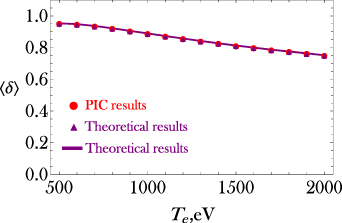
Figure 2. The effective SEE yield according to SPICE2 2D3V PIC simulations (red circles) and one-dimensional sheath theory (purple triangles and purple solid line), see equations (15) and (16) with  , as a function of the electron temperature. The PIC simulations were carried out for 16 electron temperatures that are equally spaced within 500–2000 eV and for constant plasma density of
  m−3. It is apparent that the results are indistinguishable.
Download figure:
Standard image High-resolution image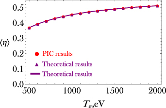
Figure 3. The effective EBS yield according to SPICE2 2D3V PIC simulations (red circles) and one-dimensional sheath theory (purple triangles and purple solid line), see equations (15) and (16) with  , as a function of the electron temperature. The PIC simulations were carried out for 16 electron temperatures that are equally spaced within
  eV and for constant plasma density of
  m−3. It is apparent that the results are indistinguishable.
Download figure:
Standard image High-resolution imageIn spite of the near-perfect agreement with PIC simulations, the computation of the double integral of equation (16) at every time step and in the entire free surface domain is computationally costly for melt motion codes. Thus, it is preferable to fit the theoretical result to a simple semi-empirical analytical expression. Since the effective yield as a function of the electron temperature is a smoothed version of the yield as a function of the incident energy, a single maximum function is sought for the effective SEE yield and a half-sigmoid function is sought for the effective EBS yield. The effective SEE yield was numerically computed from equation (16) for 500 different electron temperatures within the range of 10–5000 eV and was then least square fitted into ![$\langle\delta(T_{\mathrm{e}})\rangle = a(T_{\mathrm{e}}^{\,b}+cT_{\mathrm{e}}^{\,d})[1-\exp{(-f\,T_{\mathrm{e}})}]$](https://content.cld.iop.org/journals/0029-5515/63/2/026007/revision2/nfacaabdieqn88.gif) with
with  the unknown parameters. This procedure led to the analytical expression
with  expressed in eV. As illustrated in figure 4, there is near perfect agreement between the theoretical and semi-empirical results for the effective SEE yield, with the mean absolute relative deviations being merely
  . In a similar fashion, the effective EBS yield was also numerically computed from equation (16) for 500 different electron temperatures within the range of
  eV and was then least square fitted into
 ![$\langle\eta(T_{\mathrm{e}})\rangle = a[1-\exp{(-bT_{\mathrm{e}}^c)}]$](https://content.cld.iop.org/journals/0029-5515/63/2/026007/revision2/nfacaabdieqn93.gif) with
with  the unknown parameters. This procedure led to the analytical expression

with  again expressed in eV. As illustrated in figure 5, there is a near perfect agreement between the theoretical and semi-empirical effective EBS yield results, with the mean absolute relative deviations being merely
  .
.
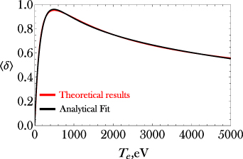
Figure 4. The effective SEE yield according to one-dimensional sheath theory (red solid line), see equation (16) with  , and according to the analytical expression (black solid line), see equation (17), as a function of the electron temperature in the range 10–5000 eV. The results are nearly indistinguishable.
Download figure:
Standard image High-resolution image
Figure 5. The effective EBS yield according to one-dimensional sheath theory (red solid line), see equation (16) with  , and according to the analytical expression (black solid line), see equation (18), as a function of the electron temperature in the range
  eV. The results are nearly indistinguishable.
Download figure:
Standard image High-resolution imageFinally, it should be strongly emphasized that the effect of the repelling wall that was excluded in the computation of the effective SEE, EBS yields should be included in the computation of the SEE, EBS current densities. The incorporation is through the incident electron current density that is calculated as  in the integration domain of
 ![$\phi\in[0,2\pi]$](https://content.cld.iop.org/journals/0029-5515/63/2/026007/revision2/nfacaabdieqn101.gif) ,
, ![$\theta\in[0,\theta_{\mathrm{M}}]$](https://content.cld.iop.org/journals/0029-5515/63/2/026007/revision2/nfacaabdieqn102.gif) ,
,  where
where  and
and  with
with  the sheath potential drop. The above calculation leads to the well-known expression for the electron current density that reads as
  . Thus, overall, we have
5.2. Semi-empirical description of the Schottky effect
The Schottky correction to the work-function  emerges only for monotonic potential profiles, i.e. outside the SCL regime, and it depends solely on the normal electrostatic field at the wall
  , which should itself depend on the plasma conditions and total effective electron emission yield
  that includes TE with the Schottky effect, SEE and EBS. Owing to the dependence solely on the total
  value and not on the distinct
  ,
,  and
and  values, in order to extract an analytical description of the wall normal electrostatic field, it is more convenient to perform PIC simulations with TE including the Schottky effect, in absence of SEE & EBS.
PIC simulations have been performed for the aforementioned OVT and IVT electron temperature—plasma density combinations and for varying surface temperatures in absence of EIEE (SEE & EBS). The latter variations lead to variations of the total effective electron emission yield through control of the TE current. In particular, 13 SPICE2 2D3V simulations have been carried out with  3400–4600 K (varying in steps of 100 K) and
  eV,
eV,  m−3 (IVT conditions) while 11 SPICE2 2D3V simulations have also been carried out with
  3400–4400 K (again varying in steps of 100 K) and
  eV,
eV,  m−3 (OVT conditions). The upper surface temperature limits in the IVT, OVT simulations are imposed by the transition to the SCL regime.
The strategy for the determination of a semi-empirical analytical expression of the normal wall electrostatic field  via the plasma parameters and the total effective electron emission yield
  is summed up in the following. (a) The scaling properties of Poisson's equation in the sheath lead to the expectation that
  should depend on the plasma conditions solely through a
  pre-factor, regardless of
  , as confirmed in figure 6. (b) As the effective electron emission yield increases, the reduced wall electrostatic field
  should monotonically decrease from
  at
at  , as dictated by classical sheath theory [3], to
  at
at  , as dictated by emissive sheath theory [18, 19]. There is no reason to expect any extrema in-between, thus a polynomial representation of
  should be appropriate. (c) A
  dataset is generated, that is based on the PIC simulations and theoretical results, which consists of
  data points. The dataset is then least square fitted into the cubic polynomial
  with
with  the unknown parameters. This procedure leads to the analytical expression
As illustrated in figure 7, there is an excellent agreement between the PIC simulations and the semi-empirical analytical expression for the wall electrostatic field as a function of the total effective electron emission yield, with the mean absolute relative deviations being merely  .
.
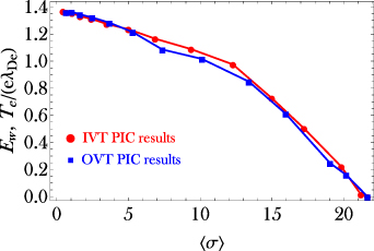
Figure 6. The reduced normal electrostatic field at the wall as a function of the total effective electron emission yield. Results from SPICE2 2D3V PIC simulations for IVT plasma conditions (red circles) and OVT plasma conditions (blue squares). The red and blue solid lines have been added to guide the eye. It is apparent that the two curves collapse on each other upon normalization with respect to  .
.
Download figure:
Standard image High-resolution image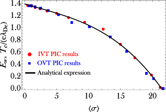
Figure 7. The reduced normal wall electrostatic field as a function of the total effective electron emission yield. Results from the semi-empirical analytical expression (black solid line), see equation (21), as well as from the SPICE2 2D3V PIC simulations for IVT plasma conditions (red circles) and OVT plasma conditions (blue squares). The high accuracy level of the proposed analytical expression is apparent.
Download figure:
Standard image High-resolution imageGiven the strong exponential dependence of the field-assisted TE on the normal wall electrostatic field, it is possible that these small deviations are strongly augmented in the course of their propagation to the thermionic current density, thus leading to large errors in the respective estimates. In order to elucidate this specific aspect, the predictions of the semi-empirical equation (21) for the emitted current density should be compared to the respective results from the PIC simulations. It should be pointed out that the  dependence leads to a strongly non-linear equation for the determination of the emitted current, given the
  definition and the
  dependence via the Schottky effect. Hence, we have
The complete non-linear problem consists of the two coupled equations (21) and (22). In particular, the emitted or escaping electron current density  is computed as follows for any plasma conditions and
  : equation (21) is substituted in the middle expression of equation (22), the rhs of equation (22) is solved numerically for
  and the solution is substituted back into the lhs of equation (22).
A detailed comparison between the semi-empirical and PIC simulation results for the escaping electron current density is featured in figure 8. It is evident that, under the IVT and OVT conditions, our semi-empirical treatment exhibits an excellent agreement with the PIC simulations. Regardless of the plasma conditions, very small deviations are only observable at the highest surface temperatures that lie near the transition to the SCL regime. At such temperatures, the total effective electron emission yield is very high and the wall electrostatic field is close to zero, thus the Schottky effect is almost negligible.
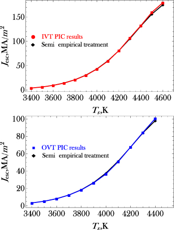
Figure 8. Escaping electron current density as a function of the surface temperature. Results from the semi-empirical treatment (black diamonds and solid line), see equations (21) and (22), as well as from SPICE2 2D3V PIC simulations for IVT plasma conditions (red circles and solid lines, top) and OVT plasma conditions (blue squares and solid lines, bottom). The solid lines have been added to guide the eye. The high accuracy level of the semi-empirical treatment is apparent.
Download figure:
Standard image High-resolution image5.3. Semi-empirical description of the limited escaping current density
In the absence of EIEE, it has been numerically demonstrated, on the basis of the analytical model developed by Takamura et al [19], that the limited value of the escaping thermionic current density in the SCL regime exhibits a very weak dependence on the thermionic electron energy distribution [20, 23]. In the present case where TE, SEE and EBS all contribute to the electron emission, the aforementioned fact implies that the limited value of the escaping thermionic current density should remain nearly the same for multi-emissive SCL sheaths as for pure thermionic SCL sheaths. The only difference between these two cases concerns the surface temperature at which the SCL transition takes place, which should be shifted towards lower surface temperatures due to the  -independent contribution from SEE & EBS. Therefore, the established semi-empirical expression for the limited escaping current density should still be highly accurate [23, 24], but it now refers to the total escaping emitted current density (TE+SEE+EBS) and not to the escaping thermionic current density. This discussion is only valid for normal inclination angles, since there should be a strong energy distribution dependence of prompt re-deposition on the magnetic field inclination angle [21]. At normal inclinations, the semi-empirical expression of interest has the simple form [23, 24]

where  denotes the plasma electron thermal velocity.
In the course of our first investigation of ITER-relevant multi-emissive sheaths [24], it was already revealed that equation (23) remains very accurate. In the present study, we shall further substantiate this claim with additional computational evidence. In particular, 8 SPICE2 2D3V simulations (TE+SEE+EBS) have been carried out within the ITER-relevant SCL regime; 3 simulations for  eV,
eV,  m−3 and
  K (IVT conditions) plus 5 simulations for
  eV,
eV,  m−3 and
  K (OVT conditions). All the results for the limited escaping current density have been plotted in figure 9. It is clear that the semi-empirical expression remains very accurate, but still falls outside the 5σ range. The level of accuracy is higher for OVT conditions, whereas there seems to be a consistent overestimation for IVT conditions.
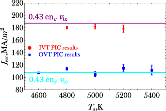
Figure 9. Escaping electron current density as a function of the surface temperature within the space-charge limited regime. Results from SPICE2 2D3V PIC simulations for IVT plasma conditions (red circles) and for OVT plasma conditions (blue squares) together with the predictions of the semi-empirical expression of equation (23) for IVT plasma conditions (purple solid line) and for OVT plasma conditions (blue solid line). The error bars denote ± five standard deviations of the total escaping electron current density, which is calculated from the distinct standard deviations of the escaping TE, SEE and EBS current densities. The latter are computed from the fluctuating PIC output after convergence.
Download figure:
Standard image High-resolution image5.4. Benchmarking of the semi-empirical descriptions
In section 5.1, the semi-empirical description of the SEE and EBS escaping current densities, valid for both monotonic and non-monotonic sheath potential profiles, was introduced and benchmarked against PIC simulations in absence of TE. In section 5.2, the semi-empirical description of the field assisted TE escaping current density, that is valid only for monotonic sheath potential profiles, was introduced and benchmarked against PIC simulations in absence of EIEE. In section 5.3, the semi-empirical description of the overall limited escaping current density, that is valid only in the SCL regime, was introduced and benchmarked against TE+SEE+EBS PIC simulations. In the present section, the semi-empirical expressions for the SEE, EBS and field assisted TE escaping current densities will be benchmarked against TE+SEE+EBS PIC simulations of the monotonic sheath potential regime, completing the validation of our approach. This final validation exercise is of particular importance, since it concerns independent PIC results that have not been utilized during the construction of the semi-empirical treatment.
In this case, the non-linear equation for the total effective electron emission yield  should also consider the SEE and EBS contributions. In particular, equation (22) is no longer valid and should be substituted with
The difference between equations (22) and (24) lies in the rhs term. It originates from the fact that the normal wall electrostatic field depends on the total effective electron emission yield  , while the field assisted TE escaping current density depends on the effective TE electron emission yield that is defined by
  in the presence of EIEE, see the rhs of equation (24), and by
  in absence of EIEE, see the rhs of equation (22).
The complete non-linear problem consists of the two coupled equations (21) and (24). For any plasma conditions and any surface temperature, the calculation proceeds as follows. The effective SEE and EBS yields are first computed from equations (17), (18) and the respective escaping current densities are computed from equations (19) and (20). The total effective electron emission yield is then computed by substituting for equation (21) in the middle expression of equation (24) and numerically solving the rhs of equation (24). Finally, this enables the computation of the effective TE electron emission yield either from the Schottky expression or the yield budget.
PIC simulations of the multi-emissive ITER-relevant sheath (TE+SEE+EBS) in the monotonic sheath potential regime have been carried out for the aforementioned OVT and IVT electron temperature—plasma density combinations and varying surface temperatures. In particular, six SPICE2 2D3V simulations have been performed with  3600–4600 K (varying in steps of 200 K) and
  eV,
eV,  m−3 (IVT conditions) while five SPICE2 2D3V simulations have also been carried out with
  3600–4400 K (again varying in steps of 200 K) and
  eV,
eV,  m−3 (OVT conditions). As per usual, the upper surface temperature limits in the IVT and OVT simulations are imposed by the transition to the SCL regime.
The comparison between the semi-empirical treatment and the PIC simulations is featured in figure 10 for the three partial escaping current densities (SEE, EBS, TE) and the normal wall electrostatic field as well as in figure 11 for the total escaping electron current density. In all cases and for all quantities, the agreement is truly excellent lending confidence to our simple practical approach. As far as the total escaping current density is concerned, which is the most important quantity in view of metallic melt motion applications: the maximum and mean absolute relative errors are  and
and  for the IVT conditions, while the maximum and mean absolute relative errors are
  and
and  for the OVT conditions. Figure 11 also demonstrates the large total escaping current density errors that would have been introduced, had the multi-emissive ITER intra-ELM sheath been treated similar to the pure thermionic intra-ELM sheath. In the IVT case, at 3600 K, the full multi-emissive treatment leads to a 6.1 × larger escaping current density than the pure thermionic treatment. This ratio monotonically decreases with the surface temperature and becomes 1.3 × at 4600 K. In the OVT case, at 3600 K, the multi-emissive treatment leads to a 4.3 × larger escaping current density than the pure thermionic treatment. The ratio again decreases with the surface temperature and becomes 1.4 × at 4400 K. This monotonic decrease with increasing surface temperature, reflects the respective monotonicity of the normal wall electrostatic field. As discussed in 5.3, the difference between the multi-emissive and thermionic treatment becomes negligible, only once the SCL regime is reached.

Figure 10. (a) Escaping SEE current density, (b) escaping EBS current density, (c) wall electrostatic field & (d) escaping thermionic current density as a function of the surface temperature  or the total effective electron emission yield
  within the monotonic potential profile regime of the multi-emissive sheath. Results for IVT plasma conditions (top panel) and OVT plasma conditions (bottom panel) from SPICE2 2D3V PIC simulations (red circles—IVT and blue squares—OVT) together with the predictions of the semi-empirical treatment (black solid line). The agreement is excellent.
Download figure:
Standard image High-resolution image
Figure 11. Escaping electron current density as a function of the surface temperature  within the monotonic potential profile regime of the multi-emissive ITER-relevant sheath. Results from SPICE2 2D3V PIC simulations for IVT plasma conditions (red circles, top panel) and for OVT plasma conditions (blue squares, bottom panel) together with the predictions of the semi-empirical treatment (black solid lines) and the predictions of the Richardson–Dushman formula (black dashed lines). There is a truly excellent agreement between our treatment and the simulations.
Download figure:
Standard image High-resolution image
In stark contrast to the effective SEE and EBS yields that only depend on the electron temperature and have been fitted to simple analytical expressions, the solution of the full non-linear problem for the effective TE electron emission yield depends on the plasma density, the electron temperature and the surface temperature. Thus, it cannot be fitted to a practical closed-form expression. As a consequence, the introduction of multi-dimensional tabulations is rather inevitable for the cost-effective numerical implementation of the effective TE yield in melt dynamics codes.
6. Discussion and future work
The multi-emissive sheaths that surround hot W surfaces during ITER intra-ELM periods are characterized by the importance of EIEE (SEE and EBS) and the strong entanglement between TE and field electron emission (primarily within the Schottky regime). In addition, in the case of normal magnetic field inclination that is relevant for exposed leading edges, the transition to the space-charge limited regime takes place at surface temperatures much higher than the W melting point. This implies that the monotonic potential profile regime is most relevant for melt motion applications, in contrast to contemporary devices where the space charge limited regime is typically reached prior to the W melting point. The escaping electron current density in the monotonic potential profile regime has strong dependence on the electron emission model and especially on the rather uncontrollable surface conditions of the plasma-facing components. Hence, this could lead to potentially large unavoidable uncertainties in the output of macroscopic melt motion codes that will be evaluated in the future for concrete ITER scenarios.
On the basis of systematic PIC simulations with the 2D3V SPICE2 PIC code, recently equipped with a state-of-the-art W electron emission model, a highly accurate semi-empirical analytical treatment has been constructed that describes the escaping electron current density from multi-emissive ITER sheaths. The description consists of analytical expressions for the effective SEE yield and for the effective EBS yield as functions of the electron temperature as well as an analytical expression for the normal wall electrostatic field as function of the total effective electron emission yield. The stabilizing negative feedback loop, that is generated by the dependence of the Schottky effect on the electrostatic field, is ultimately translated to a non-linear system of equations that can be easily solved numerically. Extensive validation against additional PIC simulations confirmed the remarkable accuracy of the proposed semi-empirical treatment.
It should be emphasized that the applicability of the proposed semi-empirical treatment is dictated by the validity of the underlying W electron emission model [24]. The treatment of W EIEE is strictly applicable to electron temperatures above 100 eV, but it can be applied down to 50 eV without introducing substantial errors. This lower bound stems from the emergence of the neglected low-energy quasi-elastic electron reflection at the W interface [35, 64, 65]. The treatment of field-assisted TE is only applicable for  where the field is measured in V m−1 and the temperature is in K. For stronger electrostatic fields, the quantum tunneling contributions start to dominate the classical over-the barrier contributions ultimately passing over to the regime of thermally-assisted field emission [66, 67].
Future investigations will focus on the following directions. First, the collisionless picture of the multi-emissive ITER-relevant sheaths needs to be extended from normal to arbitrary (including grazing) magnetic field inclination angles. The prompt geometric re-deposition of the emitted electrons in the course of their first Larmor gyration should lead to complications in the monotonic potential profile and space-charge limited regimes, especially when taking into account the vastly different energy distributions of the three emitted electron populations as well as the strong dependence of the SEE and EBS yields on the incident plasma electron angle. Second, the effect of the finite collisionality on both multi-emissive and thermionic sheaths needs to be explored. This effect mainly concerns the Coulomb collisions of the very cold thermionic electrons regardless of the surface temperature [68] and the plasma collisions with neutrals at very elevated surface temperatures. Finally, the possible importance of other electron emission mechanisms, such as photoelectric emission for intense radiation fluxes [69] and ion-induced electron emission for very hot plasma ions or highly charged impurity ions [70], needs to be evaluated for concrete ITER scenarios.
Acknowledgment
P T and S R acknowledge the financial support of the Swedish Research Council under Grant No. 2021-05649. The present work was supported by the MEYS project CZ . This work has also been carried out within the framework of the EUROfusion Consortium and has been funded by the European Union via the Euratom Research and Training Programme (Grant Agreement No. 101052200 EUROfusion). Views and opinions expressed are however those of the authors only and do not necessarily reflect those of the European Union or the European Commission. Neither the European Union nor the European Commission can be held responsible for them. The PIC simulations reported herein have been performed at the National Computational Center IT4Innovations and Marconi-Fusion.