


Abstract
The COMPASS upgrade tokamak (Panek et al 2017 Fusion Eng. Des. 123 11–16) will be a tokamak of major radius R0 = 0.894 m with the possibility to reach high field (Bt ∼ 5 T) and high current (Ip ∼ 2 MA). The machine should see its first plasma in 2023 and H-mode plasma will be obtained from 2025. The main auxiliary heating system used to access H-mode will be 4 MW of neutral beam injection (NBI) power. The NBI will have a nominal injection energy of 80 keV, a maximum injection radius Rtan = 0.65 m and will create a population of well-confined energetic D ions. In this contribution, our modelling studies the NBI deposition and losses when a significant edge background density of neutrals is assumed. We follow the fast ions in the 3D field generated by the 16 toroidal field (TF) coils using the upgraded EBdyna orbit solver (Jaulmes et al 2014 Nucl. Fusion 54 104013). We have implemented a Coulomb collision operator similar to that of NUBEAM (Goldston et al 1981 J. Comput. Phys. 43 61) and a charge-exchange operator that follows neutrals and allows for multiple re-ionizations. Detailed integrated modelling with the METIS code (Artaud et al 2018 Nucl. Fusion 58 105001) yields the pressure and current profiles for various sets of achievable engineering parameters. The FIESTA code (Cunningham 2013 Fusion Eng. Des. 88 3238–3247) calculates the equilibrium and a Biot–Savart solver is used to calculate the intensity of the perturbation induced by the TF coils. Initial distributions of the NBI born fast ions are obtained from the newly developed NUR code, based on Suzuki et al (1998 Plasma Phys. Control. Fusion 40 2097). We evolve the NBI ions during the complete thermalization process and we calculate the amount of NBI ions loss in the edge region due to neutralizations. Results indicate the NBI losses for various injection geometries, various engineering parameters and various assumptions on the magnitude of the background neutral densities.
Export citation and abstract BibTeX RIS

Original content from this work may be used under the terms of the Creative Commons Attribution 4.0 licence. Any further distribution of this work must maintain attribution to the author(s) and the title of the work, journal citation and DOI.
1. Introduction
As progress is made towards the concept of a fusion reactor, it is increasingly important to monitor the various channels of heat loss of the plasma. NBI-born fast ions are usually considered well-confined. However, when the plasma reaches large densities, a significant amount of these particles can have orbits that will explore the edge (pedestal-separatrix-near SOL) region where the neutral density can be significantly higher than in the confined plasma. When the thermalization time τs becomes greater than the characteristic charge-exchange (CX) collision time τCX, a large fraction of deposited ions are neutralized. This was observed in particular in the TCV tokamak early NBI experiments [1]. The understanding of the edge content in fast ions is also relevant of resonant magnetic perturbation experiments ([2–4]) and the induced losses.
Furthermore, beam-ion acceleration during ELMs was found through direct time-resolved velocity-space measurements of fast-ion losses in the ASEDEX-upgrade tokamak [5]. A simple model suggests that the acceleration could be explained in terms of a resonant interaction between the fast-ion orbits and the parallel electric field emerging during the ELM, when magnetic reconnection is believed to take place. The finding motivates the incorporation of a kinetic description of fast particles in ELM models and may shed light on the possible contribution of fast ions to the ELM stability.
The CX-born fast neutrals can randomly end up either on the plasma facing components or be 're-ionized' as they move deeper into the plasma. These 'reborn' ions can contribute to additional core heating or end up on a loss orbit. The two fundamental times τs and τCX mentioned above can be evaluated in the pedestal region as follows (based on [6]):
with
where mD is the background plasma ion mass, mf = mD is the NBI deuterium ion mass, me is the electron mass, νe is the electron collision frequency,  is the injection energy of the fast ion (at velocity v0),
  is the critical energy (the energy at which the collision frequencies of the fast ion against background electrons and background ions are equal, Te being the temperature of the background electrons). The dependence of τs on the effective charge of the plasma Zeff was neglected. In the transport simulations, we have assumed Zeff = 1.3. The other characteristic time is expressing the lifetime of the ion before a probability of CX of 63%:
where σD(vf) is the CX cross section of the fast ion against a cold background of neutrals (for which analytical fit are found in [7]), vf is the velocity of the fast ions, n0 is the background neutral density. The average refers to the average velocity of the fast ions during their slowing down process. During simulations, it is found that the typical fast ion population originating from the NBI has an average energy of about 44 keV. To evaluate the expression, we thus use an average overall beam ion energy during slowing down of 44 keV: this yields the given numerical estimate since σD
vf (44 keV) ≃ 8.2 × 10⁻¹³ m3 s−1 as seen in appendix
Table 1. Comparison of some COMPASS upgrade predicted parameters using the 0.5D transport solver METIS and the neutral 1D transport code KN1D [8]. The top lines refer to input parameters of the codes: Bt, Ip and  (the line averaged electron density) are inputs in METIS and the boundary neutral density values
  is obtained from equation (3) and used as input in KN1D.
  is the plasma volume average density. λT
is the temperature decay length in the SOL. n0,D,ped is the neutral density at position ρpol ≃ 0.95 (pedestal top). ne,ped and Te,ped are electron density and temperature at the pedestal top. The characteristic times τs,ped (thermalization time) and τcx,ped (63% probability to undergo CX) are based on equations (1) and (2).
is the plasma volume average density. λT
is the temperature decay length in the SOL. n0,D,ped is the neutral density at position ρpol ≃ 0.95 (pedestal top). ne,ped and Te,ped are electron density and temperature at the pedestal top. The characteristic times τs,ped (thermalization time) and τcx,ped (63% probability to undergo CX) are based on equations (1) and (2).
| Main scenarios | Density scan | |||||
| A (#3400) | B (#4400) | C (#6400) | D (#13 400) | E (#13 430) | F (#13 450) | |
| Bt (T) | 2.5 | 4.3 | 5.0 | 5.0 | 5.0 | 5.0 |
| Ip (MA) | 0.8 | 1.4 | 2.0 | 0.8 | 0.8 | 0.8 |
 (1020 m−3) (1020 m−3) | 1.1 | 1.7 | 2.2 | 1.1 | 1.7 | 2.2 |
 (1018 m−3) (1018 m−3) | 1 | 2 | 4 | 1 | 2 | 4 |
 (1020 m−3) (1020 m−3) | 1.0 | 1.5 | 2.0 | 1.0 | 1.5 | 1.8 |
| Te,core (keV) | 3.2 | 4.4 | 4.7 | 5.2 | 4.2 | 2.3 |
| λT (mm) | 3.6 | 2.7 | 2.1 | 5.0 | 5.1 | 5.1 |
| n0,D,ped (1015 m−3) | 5.5 | 5 | 7 | 5.2 | 5.5 | 8 |
| ne,ped (1020 m−3) | 0.8 | 1.23 | 1.4 | 1.0 | 1.0 | 1.7 |
| Te,ped (keV) | 0.5 | 1.0 | 1.0 | 0.6 | 0.6 | 0.1 |
| τs,ped (ms) | 23 | 19 | 16 | 16 | 15 | 2.2 |
| τcx,ped (ms) | 2.2 | 2.4 | 3.0 | 2.3 | 2.2 | 1.5 |
The COMPASS upgrade tokamak [9] will be a tokamak of major radius R0 = 0.894 m with high toroidal field (Bt ∼ 5 T) and large plasma currents (Ip ∼ 2 MA). The machine will operate in H-mode from 2025. The most exposed surfaces of the plasma facing components will be tungsten-based. The main auxiliary heating system used to access H-mode will be neutral beam injection (NBI) with power up to 4 MW and a nominal injection energy of 80 keV. Whilst one of the injector box (representing 2 MW of power) will have a fixed geometry designed to inject the fast ions in the co-current direction, the other one will be stearable and able to reach typical tangency radii between Rtan ≃ −0.65 m (counter-current) and Rtan ≃ 0.65 m (co-current). Another 2 MW of additional ECRH heating will be considered in order to prevent the accumulation of heavy impurities. This overall heating power will correspond to a rather large power density (∼3 MW m−3) because of the relatively small size of the machine. At low plasma densities and in sheath limited regimes, the divertor plasma temperature could reach values of hundreds of eV. This large heat flux and temperature would cause significant damage to the tungsten-based material used for the divertor. Therefore, the tokamak will be used to establish sustainable divertor operation in conduction limited or partially detached regimes. This type of regimes are obtained at higher collisionality and separatrix densities and thus the line average plasma densities will be increased to values in the range 1–2.5 × 10²⁰ m−3. This implies the presence of a large neutral density in the scrape-off layer (SOL) [10] and thus potentially a large neutralization of fast ions in the edge region because of CX processes. Our first objective is to quantify the induced heat loads on the vessel components for planned scenarios and tangential NBI injection (Rtan ≃ 65 cm).
Another motivation for our study is to consider scenarios involving low torque induced by the NBI system, using either perpendicular or balanced (e.g. Rtan = −30 cm and Rtan = 30 cm) injection geometries. The resulting lowered plasma rotation would bring the overall experimental conditions closer to those relevant for a nuclear fusion reactor and hopefully access to an improved quiescent H-mode [11] (QH-mode). More perpendicular injection will also contribute to the reduction of the passing fast ions. This will lead to the avoidance of the excessive internal kink mode stabilization ([12, 13]) and hopefully shorter sawtooth period [14]. Finally, some experimental evidence and simulations show that there is a potential interest in developing an SOL with large neutral density: such conditions would help reduce shear flows in the SOL and thus increase the length of the footprint of the heat flux deposition on the divertor [15]. As such, in this contribution, we assess the feasibility of a large range of plasma parameters, background neutral density and NBI geometries (values of Rtan). We evaluate them in terms of power deposition efficiency and heat load on the plasma facing components.
Our estimate for the neutral background relies on existing modelling as obtained from 1D transport, using the KN1D code [8]. As boundary condition, we consider the experimental data that were obtained during the operation of the ALCATOR C-mod tokamak [16], which had similar engineering parameters to COMPASS upgrade [17]. Based on these references, the following empirical rule of thumb is used for the neutral density at the outer limiter position:

where  is the volume average density of electrons (in 1020 m−3) and
  is the molecular deuterium density at the outer mid-plane limiter (in 1019 m−3). The dividing factor of 2 was added compared with C-mod data to account for the fact that the original pressure measurement was done in a far-SOL shadowed region. Resulting values are in the range
  5 × 10¹⁸ m−3 in our study. Preliminary calculations show that no significant number of re-ionizations will occur in the beam duct in this range of neutral densities. However, higher values could compromise the access of the fast neutrals to the plasma and cause beam-blocking: this is beyond the scope of this publication.
In this paper, we focus on the consequences of the presence of this large neutral densities on the fast ions born from the NBI heating. In particular, we consider the extension of the orbit of the fast ions in the SOL with realistic values of the magnetic ripple. This paper is structured as follows. The models for the transport, equilibrium reconstruction and full-orbit evolution of the fast ions are introduced in section 2. An analysis of the effect of the NBI tangency radius is discussed in section 3 and shows the importance of the toroidal ripple in more perpendicular injection configurations. The overall results regarding the CX losses in various plasma conditions are given in section 4. Finally, section 5 summarizes the conclusions of this study.
2. Modelling of the motion of fast ions in the 3D field in the COMPASS upgrade tokamak
2.1. COMPASS upgrade plasma conditions
Detailed integrated transport modelling with the METIS code [18] yields density and temperature profiles during the flat-top with 4 MW of NBI heating and 2 MW of ECRH heating. We consider a set of equilibria covering magnetic fields and current ranging from 2.5 T to 5 T and 0.8 MA to 2 MA, respectively. The pressure and current function (RBφ ) radial profiles as obtained from the transport simulations in METIS are used as inputs for the free boundary code FIESTA [19]. The minor radius is approximately a ≃ 0.27 m.
Table 1 summarizes the relevant plasma parameters for the equilibrium considered in this study. The energy confinement time used is the one from [20] (ITERH98P(y,2)). Heat diffusion profile shapes are obtained from a Bohm gyro-Bohm scaling. The ratio of heat transport between electrons and ions is based on the ITG-TEM (ion temperature gradient-trapped electron mode) diagram. The value we retained for the temperature decay length is (based on [21]):

Here qcyl = aBt/(R0 Bpol) where Bpol is the average value of the poloidal field at the separatrix. The density decay length in the SOL is taken as λn = 1.35λT .
In this publication we refer to two categories of scenarios: the baseline scan: A, B and C (magnetic field scan at low safety factor) and the density scan: D–F (scan in increasing line-average density at 5 T and lower current).
Typical profiles obtained during the main heating phase are represented for both categories of scenarios in figure 1. These were calculated for the most tangential injection of the NBI.
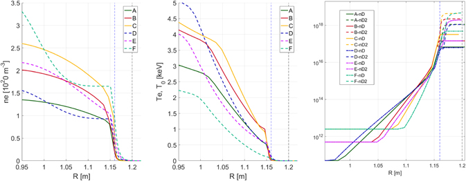
Figure 1. Left and middle: compared electron density and temperature profiles for different scenarios in COMPASS upgrade (METIS calculations). The engineering parameters of each scenarios are given in table 1. Right: resulting neutral density background profiles as obtained from KN1D [8].
Download figure:
Standard image High-resolution imageNeutral gas arises in the boundary region of tokamak plasma either because of recycling from the walls or by external gas puffing, which is often used to control the plasma density. The neutral gas in this region can be either molecular or atomic in form. Our modelling is using simple results from the KN1D code [8] that covers a large range of physical processes but only gives solution for a profile in the mid-plane. We have extrapolated to the whole poloidal plane these profiles of neutral densities by arbitrarily making them a flux surface quantity. Furthermore, we have neglected local toroidal asymmetries induced by the beam deposition (known as halo neutrals [22]).
2.2. Neutral beam injector parameters and calculation of shine-through and deposition with the NUR code
Due to geometric constrains and limited space in the openings around the torus, we are limited in tangency radius to about Rtan ≃ 0.65 m which does not allow for on-axis injection (Raxis ≃ 0.9 m). The NBIs will be located by pairs, on top of each other in each injector box (2 units of 1 MW of injection power per box). As such, they will have a vertical tilt. For simplicity, we have only considered the downward ≃5° inclination in our study. Results do not differ significantly for the paired ≃−5° upward inclination.
The neutral beam injector launches fast neutrals into the plasma. Most of them become fast ions as they collide with the plasma. The newly-developed ray-tracing code NUR calculates the initial ionization positions and velocity vector of the ions using data from [23]: its principle is given in appendix

Figure 2. Left: fraction (in%) of beam power lost to shine-through for the 6 scenarios of table 1, as a function of tangency radius (Rtan). Middle: top view of the co-current injection deposition in the case of scenario B and Rtan = 0.65 m. Right: corresponding poloidal view with the position of the markers. The total number of markers in simulations was set to 3 × 10⁵.
Download figure:
Standard image High-resolution imageBesides the tangency radius, the main beam geometry parameters used for the calculation of the deposition are the distance from the source to the tangency point (ds ≃ 5.67 m), and the elevation of the source over the mid-plane (Zs ≃ 0.425 m). We are considering a circular source grid of radius 10 cm as the source. According to the beam technical specifications, the beamlet source divergence is taken as 6.5 mrad. The beamlets are then converging at the focal point, located 5 m away from the source. This implies that the overall beam divergence will likely be higher than that of each individual beamlet. We also consider an aperture (at the narrowest part of the port) that can clamp the edges of the Gaussian distribution of the beam.
The NBI has injection energy fractions (expressed in number of deposited ions) of about 46% at 80 keV, 39% at 40 keV and 15% at 27 keV. Figure 2 illustrates the NBI deposition for the scenario with typical operational parameters (4400, scenario B). In that case, the plasma has a density of about  1.5 × 10²⁰ m−3: the shine-through is negligible and the deposition of the NBI generates a majority of passing particles with negligible first orbit losses (in an axisymmetric field).
The NUR code passes the distribution of newly born NBI ions as input to the orbit following code EBdyna in a format referred to as ion markers (corresponding for each ion to a given energy, velocity vector and position).
2.3. Biot–Savart modelling of the toroidal field and validation of EBdyna collisionless 3D orbit algorithm
Coils are described as 3D wire filaments, i.e. without thickness. The current (at least during the first second of the flat-top) is considered to be mostly localized in the inner part of the coil, as anticipated by more sophisticated ANSYS modelling. A sketch of the 3D TF wire is shown in figure 3, next to the more realistic drawing as used in ANSYS modelling. The Biot–Savart modelling discretizes a wire as a combination of very small (∼1 mm) current elements. The Biot–Savart law yields:


with B = ∇ × A, I the current (oriented along the wire) in the coil and dl the current element length. The vector r is representing the position where the field is calculated. The average value of the vacuum perturbed field is subtracted and then the axisymmetric field from the equilibrium is added in order to get the total 3D magnetic field. The solution obtained from the Biot–Savart solver is compared with a more elaborate ANSYS calculation and yields similar results. The ripple δr = (Bmax − Bmin)/(Bmax + Bmin) is evaluated to be about 0.55% at the separatrix in the mid-plane, as illustrated in figure 3.
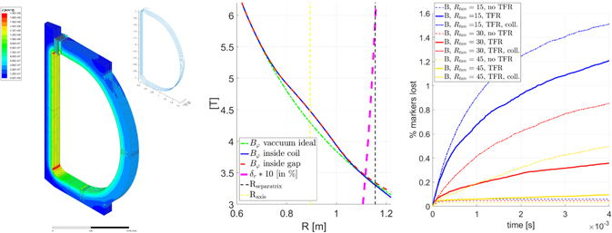
Figure 3. Left: current density distribution in the TF coil (obtained from ANSYS calculation) at the beginning of flat-top: one can notice the inhomogenous distribution on the inner side of the conductor. Insert: simplified modelling used in the vacuum Biot–Savart 3D solver, reflecting the TF current inner distribution at the beginning of the flat-top. Middle: calculation of the toroidal field and TF ripple δr = (Bmax − Bmin)/(Bmax + Bmin) for scenario B (4400). Current in the TF coil wire was then ≃0.17 MA. Right: cumulated losses (in percentage of the total number of initial markers) w.r.t. simulation time (without and with TFR; with and without Coulomb collisions) for various injection geometries in scenario B.
Download figure:
Standard image High-resolution imageEach NBI initial distribution is represented by 3 × 10⁵ markers as obtained by the NUR calculation. These markers are injected at regular time interval in the full-orbit simulation. The integrated evolution of the position of NBI D ions in the 3D TFR field is done using a grid in (R, Z, φ) repeated 16 times (the number of TF-coils). The algorithm used within the EBdyna code is given in appendix
An illustration of the evolution of the losses induced by the ripple is given on the right in figure 3. The initial distribution of the fast ions is the axi-symmetric NBI steady-state. Various parametrization of the simulation are considered. In particular, the TFR is switched off and on and the impact on the overall losses is clearly seen. When moving to collisional TFR simulation, one can notice, especially in the case of more tangential injection (Rtan = 45 cm), that the overall losses are increased due to refueling of the loss region in velocity space.
2.4. Radial ion transport due to TFR
Radial transport of trapped fast ions shows a strong correlation to the ratio of the bounce (ωb) and precession (ωφ ) frequencies [24]. In particular, significant radial excursions are found at ωb/ωφ ≃ [16/1; 16/2; 16/3] ratios. On figure 4 the collisionless motion of the trapped particles injected with Rtan = 15 cm has been studied during 1 ms in terms of losses to the wall and also their rate of change of radial position δpφ /δt (pφ being the toroidal canonical angular momentum defined in expression (B.7)). The initial distribution of markers was the steady state fast ion distribution.
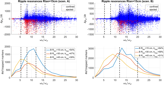
Figure 4. Left, top: evidence of ripple resonances in ωb/ωφ (vertical dashed lines) for trapped particles in the edge region (ρt ≳ 0.75) for the case of Rtan = 15 cm for scenario A. The simulation was without collisions and lasted 1 ms. Each dot represents the radial displacement at one of the 10 time stamps of the simulations. Left, bottom: distribution of number of trapped particles near the edge for each integer value of ωb/ωφ for various tangency radii (scenario A). The legend indicates the overall fraction of NBI-born trapped ions for each configuration. Right: same as left but comparing with scenario B.
Download figure:
Standard image High-resolution imageThe interaction of the NBI particles born from co-perpendicular injection geometry (e.g. Rtan = 15 cm) is complex: overlap of resonances seems to be causing enhanced stochastic losses. The increased losses at lower tangency radius are also explained by the larger amount of markers existing close the main resonances in ωb/ωφ ≃ [16/1; 16/2; 16/3], especially in the near-edge region (ρt > 0.75). The results of the TFR simulations are not changed significantly when we include the Coulomb collisions. The most noticeable effect is the enhancement of the losses due to the refilling of the loss region in velocity space (as was shown in figure 3, right).
A summary of the effect of the TFR for each scenario and injection geometry is given in the next section in table 2.
Table 2. Comparison of COMPASS upgrade predicted prompt losses (in% of beam power) and ripple-induced losses for low tangency radii (co-perpendicular injection geometry). The density scan (scenarios D–F) shows the advantage of shorter thermalization time: at lower temperatures (scenario F), slowing down is much shorter and the spread in pitch of the beam is reduced, resulting in better overall confinement of the fast ions. The comparison between scenario C (IP = 2 MA) and F (IP = 0.8 MA) shows the importance of increased plasma current in the reduction of the ripple losses.
| Main scenarios | Density scan | |||||
|---|---|---|---|---|---|---|
| 3400 (A) | 4400 (B) | 6400 (C) | 13 400 (D) | 13 430 (E) | 13 450 (F) | |
| Rtan = 15 cm (no TFR) | 2.3 | 0.5 | 0.2 | 1.5 | 0.6 | 0.1 |
| Rtan = 15 cm (TFR) | 24 | 13.2 | 0.7 | 7.6 | 15.4 | 14 |
| Rtan = 30 cm (no TFR) | 1.8 | 0.5 | 0.3 | 1.4 | 0.3 | 0.1 |
| Rtan = 30 cm (TFR) | 10 | 3.3 | 0.1 | 3.6 | 4.8 | 2.8 |
| Rtan = 45 cm (no TFR) | 1.4 | 0.6 | 0.4 | 0.9 | 0.3 | 0.02 |
| Rtan = 45 cm (TFR) | 3.4 | 0.5 | 0.0 | 1.3 | 0.9 | 0.1 |
2.5. Coulomb collisions description and comparison with NUBEAM
Expressions for the Coulomb logarithm derived from [25] for the ions and [10] for the electrons are used:

where Te is the electron temperature in eV, vthe the corresponding thermal electron velocity and vf the fast ion velocity. The saturation on velocity used on the ΛDe is a crude approximation that reflects the fact that the relative velocity of collisions remains constrained by the highest velocity of the reactants considered.
In order to completely describe the range of electron velocities available in the SOL, we use the formulas derived in [6] to express the collision rates on electrons (νb e) and on ions (νb i):

where ni indicates the background deuterium ion density,  ,
,  (vthe and vthi being the electrons and ions thermal velocities). The Maxwell integral ψ(x) and its derivative ψ'(x) are expressed as:

and for which relevant Taylor expansions can be used as given in [6]. Combined with the equation (8), this allows to express continuously the transition from vf < vthe to vf > vthe. The latter can occur in the SOL region.
Of course, the usual expression for the most common case regarding νb e is that of electrons verifying vf < vthe.
The average momentum loss is simply expressed as:

where δve = νbe vf and δvi = νbi vf refer to the norm of velocity lost during the small time δt to the electrons and the ions respectively. For completeness—as derived for the NUBEAM code in [26]—the standard deviation related to the variation of the norm of velocity during the small time δt is included as:
with

and we arbitrarily separate this spread on electrons and ions (for power deposition calculations) according to:
and
The change in norm of velocity vector after the small time δt is thus:

where  and
and  refer to random numbers following the normal distribution of mean 0, variance 1 and standard deviation 1. The energy given to the electrons and the ions are then respectively:
and

where the fluctuations related to the standard deviation have been omitted for conciseness.
In addition to energy loss, the fast ions experience perpendicular diffusion in velocity space during their thermalization (pitch angle diffusion). We can neglect the change of direction induced by the electrons (lower by a factor me/mD). The deviation of the velocity vector due to the collisions with ions is based on the characteristic time for a π/2 deviation given in [6] and is obtained by applying at each time step the change in solid angle:

with

with the remaining degree of freedom being taken randomly in a uniform distribution between 0 and 2π.
The slowing down process due to Coulomb collisions is applied to the injected markers until they reach the energy of 1.5Ti when they are then considered 'thermalized' and removed from the simulation. Their remaining energy is however still considered 'given' to the plasma ions in the total power balance. In order to be computationally efficient, we only apply the collision operators every 1 × 10⁻⁸ s which is found to be enough to reflect the local values of density and temperature along the particle orbit. A typical simulation of the 3 × 10⁵ markers lasts a few hours on a hundred processors. Once a steady-state of the beam distribution is obtained after the time τs, one can average a few subsequent outputs of the code in order to obtain a detailed map of the velocity space and density of particles. This average is typically taken over an extra ∼1.5 ms of simulation.
An illustration of the EBdyna output in the axisymmetric case is given in terms of deposited power and velocity space distribution and compared with the output from the NUBEAM code in figure 5 for scenario B. The velocity space distributions have very similar patterns in this specific example as well as in all other scenarios. The NBI density and power deposition radial profiles are in excellent agreement except in the pedestal region where it is found that the full orbit code EBdyna predicts a larger heating contribution to electrons than NUBEAM.
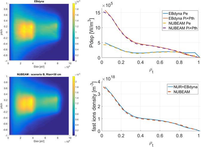
Figure 5. EBdyna and NUBEAM comparisons for scenario B, Rtan = 30 cm. No TFR or CX processes where considered. Left column: comparison of velocity space distribution of all particles between EBdyna (top) and NUBEAM outputs (bottom). Right: comparison of deposited power to electrons and ions (top) and comparison of the overall density of fast ions (bottom) after more than one thermalization time. The main qualitative difference is the difference in electron heat deposition close to the separatrix.
Download figure:
Standard image High-resolution image2.6. Charge exchange processes modelling
The charge exchange processes we have considered in our study are:

where the neutral reactants are in the ground (not excited) state. We denote σD and  respectively the cross sections corresponding to these reactions : the equations found in [7, 27] are used to model the cross section as a function of reactants relative energy is given in appendix
where  is the relevant background neutral density that are evaluated at successive instant t = jδt and v is the velocity of the ion at time t.
  refers to the reaction rate obtained by averaging the cross section values against a Maxwell–Boltzman distribution in velocities of the background neutrals or ions (see appendix
Conversely, the probability for a neutral to become ionized because of charge exchange is obtained by replacing  with the local ion density. Furthermore, a fast neutral can be re-ionized because of the ion impact ionization process:

although this process is less significant than the CX one, as is discussed in appendix
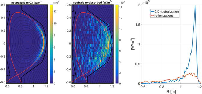
Figure 6. Illustration of the CX processes for scenario A with Rtan = 30 cm (considering only 1 MW). Left: poloidal distribution of CX radiation emission induced by the NBI. This is the density of NBI power that undergoes CX processes (neutralization). Middle: poloidal distribution of power re-deposited in the plasma because of the re-ionization processes. Right: summary figure showing the average power density taken away by neutralizations and given back by ionizations along the horizontal coordinate.
Download figure:
Standard image High-resolution image3. EBdyna outputs without charge-exchange: orbit categorization, power deposition variation with NBI tangency radius
In this section, we have deactivated all CX processes in our modelling.
3.1. Orbit categorization and orbital parameters of trapped particles
Using the steady state distribution of the NBI, we can track the resulting markers on their orbit for about 1 ms in order to discriminate their orbit categories. Such a classification is illustrated in figure 7 for the scenario B (average parameters) and the tangential injection Rtan = 65 cm and Rtan = 30 cm. The resulting classification gives us in particular the fraction of trapped particles for all configurations (scenarios and scan in Rtan). This fraction is plotted in figure 7 where we also indicate the average orbit width δr of the trapped population and their average Larmor radii.

Figure 7. Orbit categories and orbital parameters of steady-state NBI distributions. Left: scenario B: number of markers per orbit categories in several mid-plane horizontal positions. Right: top: percentage of trapped orbit for all scenarios and tangency radii. Middle: average orbit width of the trapped particles. Bottom: average Larmor radius of the trapped particles.
Download figure:
Standard image High-resolution imageIt is important to note that—in the axi-symmetric case—in considered scenarios, promptly ejected particles numbers are negligible when Rtan ⩾ 45 cm when CX processes are ignored. The losses can become however important for 0 ⩽ Rtan ⩽ 30 cm (co-perpendicular injection geometry). Table 2 gives the percentage of collisional steady-state losses for the 6 scenarios in the axi-symmetric case and compares it with the enhanced value obtained when the TFR is applied.
3.2. Power deposition profiles as a function of tangency radius
Before we move on to our detailed study of power deposition and losses when CX processes are introduced, we evaluate the NBI deposition when profiles are only the results of the Coulomb collision process when the TFR is applied. The set of profiles obtained for the total power deposited to plasma (excluding the final thermalization power) is given in figure 8 for all scenarios at Rtan = 0.65 m. We also indicate there the total amount of power deposited in the core (volume integration for positions inside ρt ≃ 0.45) and corresponding total power to the ions for all scenarios and co-injection tangency radii. We identify an optimum geometry at Rtan = 30 cm for scenarios C and E, Rtan = 45 cm for scenarios B, D and F (higher density) and Rtan = 65 cm for scenario A. The total power given to ions overall increases in all cases when we move to more tangential geometries, as core deposition is favorable to ion heating.
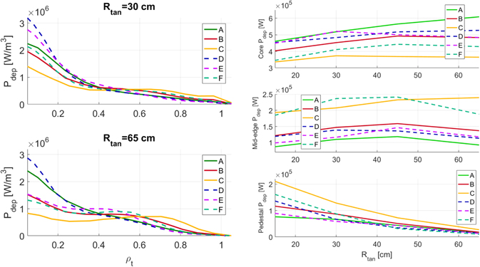
Figure 8. For 1 MW of NBI. Left: set of power deposition profiles for 2 injection geometries: top, co-perpendicular (Rtan = 30 cm) and bottom, tangential Rtan = 65 cm. Right, top: power deposited in the core (ρt < 0.4) for all scenarios as a function of tangency radius. Middle: power deposited in the mid-edge region (around ρt ≃ 0.8). Right, bottom: power deposited in the pedestal (ρt > 0.94) for all scenarios as a function of tangency radius.
Download figure:
Standard image High-resolution imageIt is found that, when we apply the CX reactions (e.g. in figure 11), the core deposited power is almost unchanged in all scenarios, all beam geometries and all realistic values of background neutral densities. As such, the right top panel in figure 8 is a realistic indication of the heating performance of each configuration.
4. NBI charge-exchange induced losses
4.1. CX neutralizations and re-ionizations: characteristic times and influence of neutral density background
Comparing the characteristic time of the CX process τCX with the thermalization time τs of the ions can give us an idea of how deeply the NBI deposition will be affected by the neutrals. This is illustrated in figure 9 where we can see that we can expect all ions with average radial position beyond ρt ∼ 0.85 to be neutralized at least once in scenarios C and F, beyond ρt ∼ 0.8 in scenarios B and E and beyond ρt ∼ 0.75 in scenarios A and D. This position thus tends to move inward with lower density, reflecting the depth of penetration of neutrals (n0 ≳ 1015 m−3). When the ratio τs/τCX is beyond 2, only few NBI fast ions can exist in the considered radial region. Comparing the scenarios, in particular C (Ip = 2.0 MA) with F (Ip = 0.8 MA), we can see the beneficial influence of higher plasma current and thus increased edge plasma density: the amount of neutrals in the edge region is reduced so that τCX is locally increased.

Figure 9. Left, top: thermalization time radial profiles of 80 keV ions. Left, bottom: radial profiles of ratios of characteristic times (τs/τCX) giving an estimate of the amount of CX reactions that can occur during the slowing down of a fast ion. The number in the caption indicates the value in the mid-edge region (ρt ≃ 0.8, corresponding to the power plotted in the right middle plot in figure 8). Right: scenario B, Rtan = 30 cm (top) and Rtan = 65 cm (bottom). Power loss w.r.t. scan in background neutral density. The reference value of boundary neutral density for scenario B is 2 × 10¹⁸ m−3. One can refer to figure 1 in order to get an idea of the neutral density profile. The multiplicative factor applied to the boundary condition corresponds to an overall multiplication of the whole profile.
Download figure:
Standard image High-resolution imageIt is of interest to study the influence of the magnitude of the background neutral density on our results since the value obtained from equation (3) is empirical. Furthermore, the magnitude of the neutral background in SOL has been observed to be correlated to modifications of the SOL transport by changes in the ExB flows (see [15]): it is thus interesting to study what are the consequences of additional content of neutrals in the SOL.
In figure 9, we selected scenario B and the tangency radii of 30 cm and 65 cm in order to do a scan in boundary value of molecular deuterium. The CX induced losses is strongly correlated to the magnitude of the neutral density. However, beyond some value, the dependence becomes weaker due to the disappearance of all fast ions in the edge region and the impossibility for the neutrals to get too deep in the core plasma. We also quantify the change in the ion losses. The tangential injection (Rtan = 65 cm) is found to be more sensitive to a further increase in neutral density: this is partly explained by the larger amount of markers initially deposited in the edge region. Furthermore, re-ionized markers tend to end up on loss orbits: the ion losses also increase with neutral density unlike in the Rtan = 30 cm case.
4.2. Simulation results: losses for each scenario and tangency radii
The CX losses are analysed for all scenario and tangency radii in the range Rtan = 15 cm to 65 cm. The results are plotted in figure 10, on the left. Two trends of CX losses can be separated based on the amount of power deposited respectively in the pedestal and mid-edge region (see figure 8, right):
- Scenarios A, C and F have low values of τs/τCX w.r.t. 1 at ρt ≃ 0.8 (figure 9): their CX losses are dominated by the deposited power in the pedestal
- Scenarios B, D and E have large values of τs/τCX at ρt ≃ 0.8 of 1 or above: their CX losses are dominated by the deposited power in the mid-edge region
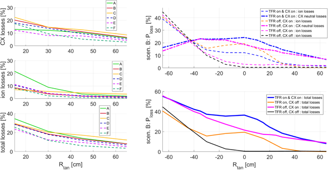
Figure 10. Left: overall losses in all scenarios for co-injection geometries. Right: impact of the TFR and CX processes in scenario B for the complete achievable range of injection geometries: Rtan = −65 cm to 65 cm. As can be derived from the plot, a reasonable choice in terms of losses for a balanced injection scenario would be a combination of Rtan = −30 cm and 30 cm. The ratio of injected power should then be lowered for the co-injection beam in order to compensate for the 38% of losses in the counter-injection case.
Download figure:
Standard image High-resolution imageThe influence of density is seen when one considers the trend within the density scan (scenarios D–F) at the most tangential co-injection geometries (Rtan ⩾ 45 cm) for which there is a low amount of power deposited in the pedestal: the drop of temperature due to the increase of density lowers τs and the lower penetration of the neutrals increases τCX: this contributes to the overall decreasing CX losses with increasing density (τs/τCX at ρt ≃ 0.8 is lowered from 2.2 (scenario D) to 0.1 (scenario F) as seen in figure 9).
On the right of figure 10, we consider a scan in beam geometry. When TFR losses are important, the overall ion orbit losses are found to be reduced by the application of the CX processes (comparing black and red line in the right figure in 10 for scenario B). This is due to the large number of neutralizations in the edge region, preventing them to be lost on longer time scales because of the TFR. The figure indicates an achievable candidate for counter injection at about Rtan = −30 cm (≃38% losses). It is of interest that balanced injection can likely be achieved in COMPASS upgrade. Indeed, the promising QH-mode observed in low momentum plasmas in DIII-D could provide a viable solution to sustaining a pedestal in a fusion reactor [28] (provided its applicability at higher heating power can be extended).
4.3. Transport simulation considering the reduction of edge deposited power
When we consider the impact of the CX losses on the plasma, one might want to know how the significant percentage of power lost (figure 11) will impact the plasma in terms of heating and performances. We have thus implemented a 'toy model' in the transport solver METIS that reproduces the edge loss and core increase pattern of the ratio of deposited power with CX-losses and without (Pdep,CX/Pdep, noCX). We find similarities between our results and those obtained in other simulations (for DIII-D) using the SPIRAL code [29]. As can be noted on figure 11, whilst the power deposited in the edge drops significantly, the power deposited in the core of the plasma is slightly increasing. That is because some of the neutrals originating from the CX processes are re-ionized in a more central location.
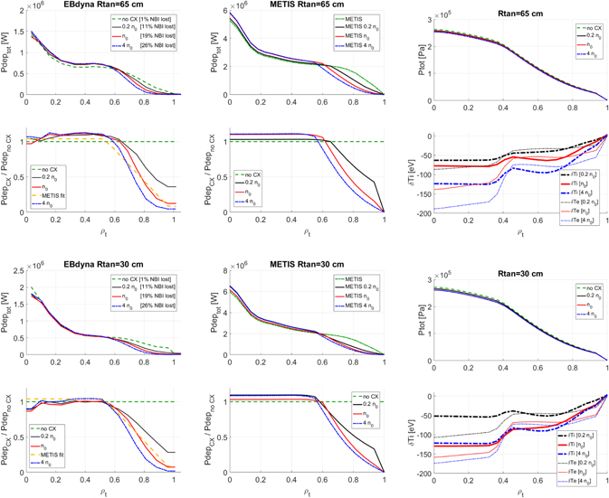
Figure 11. The top set (first and second rows) of figures is for scenario B, Rtan = 65 cm. The bottom set is for scenario B, Rtan = 30 cm. Left: power deposition profiles (top) & relative change of the power density w.r.t. simulation without CX processes (bottom) as obtained from EBdyna simulations. The profiles labelled 'n0' refer to the boundary value given in table 1 from scenario B in which  = 2 × 10¹⁸ m−3. Middle, top: power deposition of 4 MW of NBI in METIS ('toy-model') without and with the correction due to CX losses (only large losses cases were considered). Bottom: same figure as the one from left (EBdyna) but re-calculated within METIS using the model mimicking CX losses. Right: consequences of the drop in edge power deposition, in terms of overall pressure of the plasma (top) and (bottom) change in Ti (thick lines) and Te (thin lines).
Download figure:
Standard image High-resolution imageWe consider the calculation for two NBI geometries in scenario B: one with tangential injection (Rtan = 65 cm) and one with co perpendicular injection (Rtan = 30 cm). The results of this simple simulations are shown in figure 11 in the right panel. We conclude that the overall drop in plasma stored energy and temperature is relatively small, even when a very large neutral density is considered. The simple transport model predicts a uniformly radially distributed drop in ion temperature of about 5%. The losses do not seem to impact significantly the edge temperature: the drop of heat source in the edge where the gradient is constrained by the energy stored in the pedestal is not causing a drop of edge temperature but increases the cooling rate of the edge and thus decreases the core temperature. Both core electron and ion temperatures are observed to drop when increasing the neutral density (which corresponds to an increase of the edge cooling rate). The slight increase in core heating does not compensate for the lost power. As was shown previously in figure 9, the impact of a very large background neutral density (n0D2 = 4n0 ≃ 8 × 10¹⁸ m−3 case) is more problematic in the tangential injection case whilst no further drop in terms of core Ti is obtained for the co-perpendicular (Rtan = 30 cm).
4.4. Radiated power and deposition on plasma facing components
An estimate of the density of power deposited on the wall was calculated using a simplified 2D geometry of a preliminary design of the wall. The results are found in figure 12 where we have separated the incident fast neutrals and ions. Unlike the ions, the CX-born neutrals will mostly not be blocked by the outer wall limiter and will actually spread on a much larger area, that includes all of the openings in the vacuum vessel. A more detailed study of the actual power loss will be done in the future for design purposes using a complete 3D model of the components in the tokamak chamber. This is beyond the scope of this publication. We can however quantify an upper estimate for the heat flux on the limiter generated by 1 MW of NBI heating in scenario B: about 50 kW m−2 (co-injection) and 200 kW m−2 (counter-injection). These values remain well within the acceptable range of heat loads for tungsten based components (less than 1 MW m−2 in total for 4 MW of NBI heating). These heat loads and their energy distribution could be used for modelling the sputtering occurring at the surface of the limiter (and other in-vessel components) in order to evaluate the beam-induced impurity source. The simulations will also support the design of fast ion loss detectors.

Figure 12. Approximate power flux deposited on small wall elements (left and middle), scenario B, for 1 MW of NBI. The histograms on the right indicate the energy distribution of the markers lost to the outer wall limiter during ∼1.7 ms of simulation. The top figures are for co-injection at Rtan = 30 cm. Bottom: the figures are for counter-injection at Rtan = −30 cm. Figures on the left give the density of power emitted by CX processes (recombination radiation) and reflect the density of neutralizations. Figures in the middle give the neutral power flux at the wall (approximate geometry). Figures on the right side indicate the ion power flux at the 2D wall. Most of the losses are located in the mid-plane. The heat flux originating from ion losses is significant in the Rtan = −30 cm case.
Download figure:
Standard image High-resolution image4.5. Shoulder formation impact and modification of neutral density in the scrape-off layer
Shoulder formation is related to a change of filament transport in the SOL from sheath-limited to inertial regime, which is characterized by a substantial increase in density (and to a lesser extent temperature) decay length in the far SOL [30] (meaning by this denomination the region of the SOL away from separatrix by more than one conventional decay length). Increased density decay length leads to increased transport to the first wall, which can in principle lead to higher heat fluxes on the plasma-facing components. It is on the other hand possibly favourable w.r.t. The power deposition length on the divertor [31].
One of the interest of the COMPASS upgrade tokamak will be its ability to study configurations that involve a far-SOL shoulder. We have constructed an approximate shoulder configuration by multiplying the density decay length by a factor 5 in the far-SOL (for SOL positions beyond one conventional decay length as obtained from 4).
We have applied a shoulder to scenario F, which has a large Greenwald fraction of ∼0.5. The resulting profiles are given in figure 13 where we compare them with the configuration that does not have a shoulder. We have applied the KN1D modelling to both configurations and obtained different neutral background profiles.
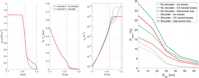
Figure 13. Left: kinetic profiles used to mimic the absence (green) or existence (red) of an SOL density shoulder in scenario F. Right: the shoulder (red curves) reduces the CX losses for all injection geometries but increases slightly the ion losses at perpendicular injection (Rtan < 30 cm).
Download figure:
Standard image High-resolution imageWe can then use the complete full-orbit modelling of EBdyna to study the difference in the CX processes because of the changes in the SOL. When a shoulder is present, the increased plasma density results in an outer ionization front away from the separatrix. This significantly reduces the neutral density in the pedestal. As a result, the edge CX losses are reduced by the presence of the shoulder.
5. Discussion and conclusions
A systematic integrated modelling approach (METIS-FIESTA-NUR-EBdyna) was developed in order to simulate NBI-born particles in a tokamak. This modelling was successfully applied to the—currently under design—COMPASS upgrade and it yielded results regarding the core power deposition, the influence of the TFR and CX induced losses. Using a simple 'toy model' of the CX losses in the fast transport solver code METIS, we have calculated that, despite the fact that the total beam losses can reach ∼20% of the injected power, the reduction of plasma energy content should not be large, since these losses occur mostly in the plasma edge and that a fraction of the CX-born neutrals actually results in increased core power deposition. In terms of the COMPASS upgrade design effort, this implies we should make sure that the PFCs are able to handle the additional heat load (typically 0.2–1 MWm−2), localized essentially on the outer wall limiter(s). Additional pumping of the mid-plane neutral could be used in order to regulate the neutral concentration in the far-SOL.
We have now developed tools in order to evaluate the fast ions and fast neutrals losses of the NBI injectors in a wide range of possible geometries and background parameters. The COMPASS upgrade tokamak will reach reactor-relevant edge plasma condition in terms of magnetic field, plasma density and neutral density. In order to study the accessibility to QH-mode as was observed in DIII-D [28], scenarios investigating low-momentum plasma (using balanced injection) will be designed and the tools described in this contribution will allow to anticipate the heat load on the plasma facing components and the complete 3D structure of the vessel.
At lower plasma current, the increase of the overall plasma density to larger Greenwald fractions will allow to investigate the density shoulder formation and its impact on the edge background neutrals and CX-NBI-losses.
Our code will allow us to accurately describe the fast ion population in the edge region of current medium size devices. As such, it can be used as an input for a detailed MHD study of the pedestal. In particular, when aiming at increasing the ELM frequency in a fusion reactor, one might want to consider a dedicated low energy NBI as a potential ELM trigger actuator: the beam would create a large fast ion beta in the pedestal region and the switch-off of the NBI would be used to destabilize the ELM [5]. Such an innovative actuator can only be efficient when we have assessed that the CX losses allow it to operate (the injection energy of such a beam should be low enough to avoid the CX process but high enough to allow the interaction with the mode). The study published in this paper paves the way to the design of experiments demonstrating the feasibility of such a control system.
Acknowledgments
This work has been carried out within the framework of the project COMPASS-U: Tokamak for cutting-edge fusion research (No. CZ.02.1.01/0.0/0.0/16_019/0000768) and co-funded by European structural and investment funds. This work was supported by The Ministry of Education, Youth and Sports from the Large Infrastructures for Research, Experimental Development and Innovations project 'IT4Innovations National Supercomputing Center—LM2015070'.
Appendix A.: Principle of NBI particle ionization with the NUR code
Electron density and temperature profiles are interpolated along the trajectories of the fast NBI neutrals (straight lines originating at the source) in order to calculate a neutral ionisation probability. The attenuation of the beam current I can be expressed as:

where I is a beam current, l is a distance along the injection direction, ne and Te are the electron density and temperature. σ is a total cross-section that is based on experimental measurements. The cross-section is including stepped ionisation processes and already averaged over the velocities of the background plasmas; it is a function of the electron temperature and electron density. As a cross-section of the ionisation process we use the one described in the paper of Suzuki [23]. Moving to the single particle, expression (A.1) can be seen as an expression for a probability of the particle to stay neutral ( ) on its trajectory.

In order to retrieve the probability one has to integrate the equation. Taking into account that probability to stay neutral in the very beginning of the path is equal to one, we get:

where the integral is taken from the source to the first intersection with the wall of the tokamak. The NUR code integrates the equation using Runge–Kutta 4th order method. Probability for particle to be in ionized state is equal to  . In order to get the ionization position. The following equation is solved:

where  is an evenly distributed random number between 0 and 1. Solving (A.4) corresponds to use a linear interpolation of the invers function of
  . When the ionization position is identified velocity vector is calculated according to the beam trajectory.
Appendix B.: EBdyna full-orbit motion of a charged particle described in tokamak cylindrical coordinates
We describe the position of a particle x in (R, Z, φ) tokamak cylindrical coordinates. In particular, the velocity vector can be decomposed along these coordinates as: v = vR eR + vZ eZ + vφ eφ . The motion of a charge particle of mass m and charge Zi is described by the evolution of velocity vector v as given by the momentum equation:

where e is the elementary charge, E the electric field and B the magnetic field.
In EBdyna, the choice has been made to solve this differential equation with the 'Boris' algorithm ([32, 33]). This algorithm is well known for its stability and performance for particle tracking in magnetic fields [34]. The 'Boris' integration method is a 'leap-frog' method: this means that the velocity is known at half time steps, whilst the position is known at integer time steps. The current time step is indicated with the superscript n. Determining the electric and magnetic fields at time step n provides an estimate for the acceleration between n − 1/2 and n + 1/2. Hence the change in velocity from vn−1/2 to vn+1/2 can be determined. The velocity vn+1/2 is then used to 'push' the particle from xn to xn+1.
We incorporate in the algorithm given below the electric field E although this feature of the code is not used in this publication. The 'Boris' method thus consists of five steps:
1. Apply the electric field E for the initial half of the step:

2. Apply a rotation of the velocity according to the magnetic field B:

with:

3. Apply the electric field E for the second half of the step:

4. Update the positions of the particles accordingly:
5. Note the ∗ symbol used for the velocity components. This has been done to indicate the components are expressed for position xn . Since the coordinate system is toroidal, the unit vectors change with position. Thus after the position update the components need a cylindrical correction to match the unit vectors at position xn+1. The change of eR and eφ during the motion is expressed with the rotation of small angle α:
with:
In order to validate the precision of our algorithm we use the exact formula for the evolution of the toroidal canonical angular momentum (pφ ) as obtained from its definition and compare it to the one obtained by evolving pφ using an exact formulation based on the vector potential. Essentially we compare the output of:

with the integrated time evolution of:

where AR
, AZ
and Aφ
are the components of the magnetic vector potential. The relative error  on the particle evolution remains below 0.1% for all markers during 4 ms collisionless 3D simulations.
Appendix C.: Charge-exchange cross sections and rates
The considered CX process neutralization of fast ions are the ones on background atomic neutrals (cross section σcxD) and molecules (σcxD2):

where we have neglected the reactions with excited states and considered all reactants in their ground state (details in [35] or [7]).
Regarding the re-ionization of CX neutrals, we consider the first two reactions below: the CX with background ions and the impact ionization reactions (cross section σi) on background ions whilst the impact ionization on electrons (third reaction) is neglected since its cross section is at least one order of magnitude lower at the considered energies:

where we have again neglected the reactions with excited states and considered all reactants in their ground state.
The integration of the cross-section on a Maxwellian distribution for given beam velocity vb and background temperature T0 was obtained by integrating twice, first along the Maxwellian in the direction of the collision and then on the Maxwellian in the plane perpendicular to the direction of collision. This writes as:
where  is the relative kinetic energy of the reaction. The integration is easily treated numerically and yields a table that is accessed by the code through a logarithmic scale in beam energy and neutral temperature. The rates of the three above implemented processes (σcxD2
v,
is the relative kinetic energy of the reaction. The integration is easily treated numerically and yields a table that is accessed by the code through a logarithmic scale in beam energy and neutral temperature. The rates of the three above implemented processes (σcxD2
v,  , and
, and  ) are plotted in figure 14 where, regarding the CX process on molecules, only the cold D2 approximation has been considered. These rates are tabulated on a log scale inside the code and interpolated for all markers at each evaluation of the collision processes (every ∼10−8 s).

Figure 14. Rates of the main reactions of neutralizations and ionizations occurring during the NBI slowing down and power deposition as a function of the energy of the fast particle (Eb) in eV. The black curve is the CX rate with molecular deuterium σcxD2
v. The full line coloured curves are for the CX rate  . The dashed coloured curve are impact ionization rates (
 ). The legend indicates the colour of the temperature of the relevant background considered (molecular D or ions). The three vertical green dashed lines indicate the three injection energies of the NBI.
Download figure:
Standard image High-resolution image