
Abstract
Three-dimensional (3D) simulations via molecular dynamics (MD) show that the brittle or ductile behavior of the atomistic samples with the edge crack (001)[110] (crack plane/crack front) depend on size of the self-similar atomistic crystals. Since the basic continuum predictions concerning cracks do not consider the random thermal atomic motion, we are restricted in this study to MD simulations with initial temperature of 0 K. For all samples tested, the crack initiation is brittle. However, the subsequent crack growth can be inhibited by twin formation on oblique planes {112}, crack branching along {011} planes and new dislocation emissions on {123} slip planes and the final fracture can also be then ductile, which depends predominantly on the thickness of the atomistic sample. The representative quantity, the atomistic fracture toughness initially increases with increasing sample thickness and later saturates near Griffith level for plane strain state along the crack front. The tested loading rates are equivalent to a cross head speed of 0.833 · 10−4 m s−1 used in one our previous experiment. These new MD results comply with the stress analysis performed by the anisotropic linear fracture mechanics (LFM) and with some experimental observations.
Export citation and abstract BibTeX RIS

Original content from this work may be used under the terms of the Creative Commons Attribution 4.0 licence. Any further distribution of this work must maintain attribution to the author(s) and the title of the work, journal citation and DOI.
1. Introduction
The brittle versus ductile behavior of materials is continuously investigated - see the regular world international ICF (e.g. ICF15, Atlanta 2023, USA) and European ECF conference on fracture (e.g. ECF23, Madeira 2022, Portugal), since the topic is very important for engineering applications. The studied crack orientation is important as well since the plane (001) is the most common cleavage plane observed in bcc iron based materials, including ferritic steels for nuclear engineering [1]. It is known that the dangerous brittle fast fracture usually occurs at low temperature or higher loading rates. A review concerning the influence of temperature and of loading or strain rate on ductile or brittle behavior of materials and fracture toughness one can find e.g. in [2].
Molecular dynamic (MD) simulations of crack behavior bring important information on how the crack itself can contribute to ductile or brittle behavior under a given external loading. The processes generated by the crack itself (such as dislocation emission, crack initiation, twinning, etc) are very fast (as this study also documents), and therefore information on these crack tip processes is difficult (or impossible) to obtain from experiments. Such information can be gained via three-dimensional (3D) atomistic simulations by molecular dynamics technique [3]. However, the MD simulations have also some limitations. A review on limitations and capabilities of MD simulations is presented in [4]. In relation to experiments, one problem is that there is impossible to realize in MD true strain rates from fracture experiments for a large time consumption (10+14 time steps in MD is needed [5] to model a fast fracture from experiments). For that reasons, such MD studies are rare. As mentioned in the recent study [5], for a qualitative assessment of the influence of strain rate, one can overcome the problem using an elasto-dynamic concept from linear fracture mechanics (LFM). Here the influence of strain rate is treated via an equivalent loading rate (dP/dt)exp = (dP/dt)MD, where t means the time, P means the resultant force acting on the specimens of similar geometries in experiment (index 'exp') and in MD (index 'MD'). The geometry and orientation of the considered 3D atomistic and experimental specimens are shown in figure 1, where the resulting force P acts along the sample length L.
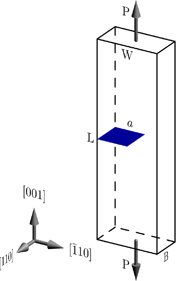
Figure 1. Scheme of loading and the orientation of bcc iron crystals with the initial edge crack a.
Download figure:
Standard image High-resolution imageHere, P denotes the resulting force; L marks the length, W is the width and B is the thickness.
Recent MD study [6] in fcc nickel show that fracture toughness may depend on the thickness B of the 3D atomic sample, namely when crack initiation is accompanied with dislocation emission at the free sample surfaces. Dislocation emission at the free sample surfaces (LW in figure 1) occurs also at our edge crack (001)[110] in bcc Fe loaded in mode I, as presented in [5]. However, we tested in [5] only one atomistic 3D specimen of minimum thickness B consisting of 30 layers (110) along the crack front [110] in figure 1. As discussed in [5], this thickness is sufficient to describe well dislocation emission in MD by the continuum predictions presented in [7]. In this paper we will utilize the elasto-dynamic concept from [5], but unlike [5], this paper is devoted to a new topic, namely to effect of sample size on the brittle or ductile behavior in MD simulations that are focused to fracture experiments on bcc iron crystals with edge crack (001)[110] loaded in mode I with a faster cross head speed of 0.833 · 10−4 m s−1 (5 mm min−1).
Magnitude of the sample thickness B may affect plane stress versus plane strain state in the 3D atomistic sample and consequently also the processes generated by the crack itself in MD simulations. Magnitudes of the sample length L and sample width W may also affect MD results since the crack and the dislocations generated by the crack have the stress field of a long range. Also, the crack initiation and dislocation emission (or generation of other defects by the crack) in MD sample will generate the elastic waves that travel to sample surfaces, where they reflect back to the crack front and may influence the further crack development in dependence on L, W, and B, etc
The aim of this paper is to examine and explain the mentioned size effects in new MD simulations via parallel processing using OpenMP [8] in 3D atomic samples of various dimensions, including the influence of the sample thickness B on crack behavior. To assess the stress state and the associated continuum predictions, we present also additional calculations of the stress on the atomistic level, based on an interplanar concept published in [9]. Since the basic continuum predictions concerning cracks do not consider the random thermal atomic motion, we are restricted in this study to MD simulations with initial temperature of 0 K. Unlike [5], we investigate here a different geometry of the specimens from fracture experiments in [10], namely with a smaller ratio L/W. The details are given in section 2. At the end of the section 3 we discuss not only the advantages but as well the limitations of the MD simulations.
2. MD simulations
The dimensions of the tested 3D atomistic samples are presented in table 1. The cracked crystals from figure 1 consists of M planes (001) in the direction x2 = [001] parallel with the length L, further N planes  in the direction x1
=
in the direction x1
=
![$[\bar{1}10]$](https://content.cld.iop.org/journals/1402-4896/98/12/125974/revision2/psad0d67ieqn2.gif) (the width W) and J planes (110) along the crack front, parallel with the direction x3 = [110] and the sample thickness B. The total number of atoms in such sample is NA = (M N/2) J. The initial edge crack (001)[110] of the length a in the middle (at L/2) was created by cutting the interatomic bonds in the [001] direction along the crack surface (i.e. between the layers M/2 and M/2+1). The interactions across the initial crack planes (001) were not allowed during the MD simulations. The relative dimensions of the atomistic samples B/W and L/W correspond to the relative dimensions of the specimens treated in the fracture experiments in [10], so that the boundary corrections factors FI (a/W) and fI (a/W) staying in LFM at the stress intensity factor KI [11] and the T-stress [12, 13] are the same in MD, LFM and in our next planed experiment. The true length L, the width W and the thickness B of the individual tested 3D atomistic samples correspond to L = M d001, W = N d110
, B = J d110, where d001 = a0 /2, d110 = a0 √2/2 are the interplanar distances between the planes {001} and {110} in the bcc lattice with the lattice parameter a0. We should note that the specimens for fracture experiments in [10] are shorter (with smaller length L) than in the first experiment treated in [5]. In this paper we consider the sample geometry by [10] because only such single crystals are currently available for us.
(the width W) and J planes (110) along the crack front, parallel with the direction x3 = [110] and the sample thickness B. The total number of atoms in such sample is NA = (M N/2) J. The initial edge crack (001)[110] of the length a in the middle (at L/2) was created by cutting the interatomic bonds in the [001] direction along the crack surface (i.e. between the layers M/2 and M/2+1). The interactions across the initial crack planes (001) were not allowed during the MD simulations. The relative dimensions of the atomistic samples B/W and L/W correspond to the relative dimensions of the specimens treated in the fracture experiments in [10], so that the boundary corrections factors FI (a/W) and fI (a/W) staying in LFM at the stress intensity factor KI [11] and the T-stress [12, 13] are the same in MD, LFM and in our next planed experiment. The true length L, the width W and the thickness B of the individual tested 3D atomistic samples correspond to L = M d001, W = N d110
, B = J d110, where d001 = a0 /2, d110 = a0 √2/2 are the interplanar distances between the planes {001} and {110} in the bcc lattice with the lattice parameter a0. We should note that the specimens for fracture experiments in [10] are shorter (with smaller length L) than in the first experiment treated in [5]. In this paper we consider the sample geometry by [10] because only such single crystals are currently available for us.
Table 1. Notation (No) of the atomistic sample, number of atomic layers (N in ![$[\bar{1}10],$](https://content.cld.iop.org/journals/1402-4896/98/12/125974/revision2/psad0d67ieqn3.gif) M in [001], J in [110]) in the tested samples from figure 1, total number of atoms NA, initial crack length a / d110, ratio a /W and the boundary correction factors FI
(a/W), where the sample width is W = N d110 and d110 is the interplanar distance between {110} planes. Static value of the Griffith stress is calculated as σG
= KG
/ FI (π a)1/2 with KG = 0.835 MPa m1/2 for plane (pl) stress and KG = 0.9115 MPa m1/2 for plane (pl) strain and the potential in use.
M in [001], J in [110]) in the tested samples from figure 1, total number of atoms NA, initial crack length a / d110, ratio a /W and the boundary correction factors FI
(a/W), where the sample width is W = N d110 and d110 is the interplanar distance between {110} planes. Static value of the Griffith stress is calculated as σG
= KG
/ FI (π a)1/2 with KG = 0.835 MPa m1/2 for plane (pl) stress and KG = 0.9115 MPa m1/2 for plane (pl) strain and the potential in use.
| No | N | M | J | NA | a /d110 | a /W | FI (a/W) | σG (GPa) pl. stress | σG (GPa) pl. strain |
|---|---|---|---|---|---|---|---|---|---|
| B30 | 150 | 600 | 30 | 1 350 000 | 64 | 0.4267 | 2.2454 | 1.84 | 2.01 |
| B40 | 200 | 800 | 40 | 3 200 000 | 84 | 0.4200 | 2.2255 | 1.62 | 1.77 |
| B50 | 250 | 1000 | 50 | 6 250 000 | 106 | 0.4240 | 2.2374 | 1.44 | 1.57 |
| B60 | 300 | 1200 | 60 | 10 800 000 | 128 | 0.4267 | 2.2454 | 1.30 | 1.42 |
| B70 | 350 | 1400 | 70 | 17 150 000 | 148 | 0.4229 | 2.2341 | 1.22 | 1.33 |
As in previous studies, we use in MD a many-body potential for Fe-Fe interaction from table 2 in [14] with the lattice parameter a0 = 0.28665 nm (2.8665 Å) and with the basic elastic constants given in [14]. Surface formation energy γ001 and the different elastic coefficients C for plane stress and plane strain state are given in [5]. The corresponding values of Griffith stress intensity factors, calculated from the relation 2 γ001 = C (KG)2 are given table 1.
Table 2. MD results with 3D atomistic samples B30-B70 of different size (see table 1). Here, dP/dt denotes the loading rate, dσ/dt is the corresponding stress rate applied in MD at BW borders, ΔtG is an informative quantity about the time required to reach Griffith load σG for plane stress, te is the time of the surface dislocation emission  in MD, ti is the time of crack initiation, tf is the time of final fracture. The quantities σi
, σe and σf correspond to applied stress level at the time ti
, te and tf during the linear time loading
in MD, ti is the time of crack initiation, tf is the time of final fracture. The quantities σi
, σe and σf correspond to applied stress level at the time ti
, te and tf during the linear time loading  Further, RKmax denotes the maximum value on the atomic tensile curve RK - t, the associated stress is
  and CODf is the crack opening in the lower half of the crystal at the final fracture time tf.
| Sample No | dP/dt (kN s−1) | dσ/dt (GPa/h) | ΔtG/h | te / h | σe (GPa) | ti / h | σi (GPa) | tf / h | σf (GPa) | CODf Å | RKmax( 10−6N) | σMD (GPa) |
|---|---|---|---|---|---|---|---|---|---|---|---|---|
| B30 | 4.50 | 3.68/15120 | 7560 | 6869 | 1.67 | 6966 | 1.70 | 11450 | 2.79 | 45 | 0.3219 | 1.74 |
| B30 | 5.85 | 3.68/11630 | 5815 | 5953 | 1.88 | 6049 | 1.91 | 9925 | 3.14 | 46 | 0.3148 | 1.70 |
| B40 | 4.50 | 3.22/23520 | 11833 | 10127 | 1.39 | 10282 | 1.41 | 21168 | 2.90 | 125 | 0.5812 | 1.77 |
| B40 | 5.85 | 3.22/21732 | 10933 | 9677 | 1.43 | 9827 | 1.42 | 21732 | 3.22 | 170 | 0.5703 | 1.73 |
| B50 | 4.50 | 2.90/33096 | 16434 | 13746 | 1.21 | 13976 | 1.23 | 30155 | 2.64 | 163 | 0.8124 | 1.58 |
| B50 | 5.85 | 4.32/37923 | 12641 | 11522 | 1.31 | 11728 | 1.34 | 27916 | 3.18 | 234 | 0.8109 | 1.57 |
| B60 | 4.50 | 3.90/64091 | 21364 | 18325 | 1.12 | 18643 | 1.13 | 40774 | 2.48 | 177 | 1.2146 | 1.64 |
| B60 | 5.85 | 3.90/49302 | 16434 | 14545 | 1.15 | 14803 | 1.17 | 32968 | 2.61 | 217 | 1.0114 | 1.37 |
| B70 | 5.85 | 3.90/67110 | 20993 | 17948 | 1.04 | 18320 | 1.07 | 41969 | 2.44 | 233 | 1.4110 | 1.40 |
Before the loading, surface relaxation in the atomistic 3D samples is performed (as in our previous studies) to bring the system into equilibrium and to avoid the influence of surface relaxation on crack tip processes in the subsequent MD simulations with the loaded crystals - see figure 1.
No periodic boundary conditions are utilized in the MD simulations, i.e. the LW and BL surfaces in figure 1 are free of external forces, like in fracture experiments with SEN (single edge notched) specimens loaded in tension mode I (i.e. in the [001] direction as in [10] and figure 1).
The relaxed atomistic 3D samples are loaded after the surface relaxation, i.e. at initial temperature of ∼0 K and further thermal atomic motion is not controlled. Newtonian equations of motion for the individual atoms are solved in the all 3 directions x1, x2 x3, using a stable time integration step h = 1 × 10⁻¹⁴s.
The loading rates are introduced in MD via the relation (dP/dt)exp = (dP/dt)MD and they differ from [5] due to the different length L of the experimental specimens in [10]. The experimental elastic estimate is (dP/dt)exp = E BW (dV/dt)/L, where V is the relative displacement in the L-direction between the top and bottom surfaces. This is calculated with Young modulus E = 1/s22 = 135 GPa for plane stress or with E = 1/A22 = 175.5 GPa for plane strain, further with thickness B∼2 mm, width W∼10 mm and length L∼50 mm as in the experiment [10] and for the cross head speed VE = dV/dt = 0.833 · 10−4 m s−1 (5 mm min−1). In this study, the elastic approach corresponds to either dP/dt = 4.5 kN s−1 or to dP/dt = 5.85 kN s−1, which differs from [5] significantly. These values are used to determine the loading rate (dσ/dt) in MD (see table 2) via relations dP/dt = (dσ/dt)(BW)MD where B = J d110 , W = N d110 follow from table 1. For example, if the crack in the sample B70 of the initial length a = 148 d110 from table 1 is considered, then for the ratio a/W = 0.4229 one obtains from [11] the boundary correction factor FI = 2.2341 and from the known LFM relation (KG
= FI
σG
 ) Griffith stress σG = 1.22 GPa for plane stress conditions (with KG = 0.835 MPa m1/2) is obtained—see table 1. The rise time ∆tG (∆tG = tG
– 0) needed to reach this critical level ∆σG = (σG – 0) = 1.22 GPa with loading rate (dP/dt)exp = 5.85 kN s−1 is given by the relation 5.85 kN s−1 = ∆σG
(BW)MD /∆tG
, which represents 20993 h , where h = 1 × 10⁻¹⁴s is the used time step in MD - see table 2. If plane strain state is considered, σG in table 1 is larger since KG = 0.9115 MPa m1/2 for plane strain is larger. As well the loading rate is dP/dt = 5.85 kN s−1 and the stress rate dσ /dt in table 2 are higher for plane strain due to the relation 5.85 kN s−1 = (BW)MD
dσ / dt. These examples and the other are treated in the section 3.
) Griffith stress σG = 1.22 GPa for plane stress conditions (with KG = 0.835 MPa m1/2) is obtained—see table 1. The rise time ∆tG (∆tG = tG
– 0) needed to reach this critical level ∆σG = (σG – 0) = 1.22 GPa with loading rate (dP/dt)exp = 5.85 kN s−1 is given by the relation 5.85 kN s−1 = ∆σG
(BW)MD /∆tG
, which represents 20993 h , where h = 1 × 10⁻¹⁴s is the used time step in MD - see table 2. If plane strain state is considered, σG in table 1 is larger since KG = 0.9115 MPa m1/2 for plane strain is larger. As well the loading rate is dP/dt = 5.85 kN s−1 and the stress rate dσ /dt in table 2 are higher for plane strain due to the relation 5.85 kN s−1 = (BW)MD
dσ / dt. These examples and the other are treated in the section 3.
The loading procedure in mode I (in the x2 = [001]-direction) is the same as in our previous studies: loading is realized by applying external forces F2(li, t) = σ(t) a0 2/6 to each atom li in the 6 upper and lower BW surface layers (001) in figure 1. The loading is linear in time (according to the calculated rate dσ/dt in table 2) up to final fracture in each MD run.
Static solution at an applied constant stress in section 3.1.1 is obtained from MD simulation using the critical damping in the Newtonian equation of motion for the basic longitudinal vibrations of the atomistic sample described in section 3.2. (The same technique is used for surface relaxation under zero applied stress.)
Similar to all our previous studies, after the loading and during the time integration of Newtonian equations, the global energy balance is monitored each time step, as well as the total number of the interactions LINT , the crack opening displacements COD(t) and the instantaneous crack length (KRACK) in the middle layer at B/2, which define the time of crack initiation ti and consequently the level of external loading σi
= σ (ti) and the stress intensity  at the crack initiation. To reveal the time te of the surface dislocation emission into oblique slip systems
  mentioned in [5], we monitor each time steps also the relative surface displacements at the crack tip in the first surface layer (110) (LW in figure 1). The relative shear displacement in the direction of the Burgers vector b = a0√3/2
 ![$[11\bar{1}]$](https://content.cld.iop.org/journals/1402-4896/98/12/125974/revision2/psad0d67ieqn10.gif) on (011) slip planes during dislocation emission is denoted further as U10 and this concerns the 'fixed' crack tip atom (index 0) and the 'moving' atom below the crack tip (index 1), as defined in [5] by equation (2). Similar to crack initiation we then determine
on (011) slip planes during dislocation emission is denoted further as U10 and this concerns the 'fixed' crack tip atom (index 0) and the 'moving' atom below the crack tip (index 1), as defined in [5] by equation (2). Similar to crack initiation we then determine  and
and 
The atomic coordinates and the local number of interatomic interactions KNT(li ) at all the individual atoms li are printed only at selected time steps because of graphical processing of MD results.
Similar to dependencies P- t and P - ∆L monitored in fracture experiments (e.g. [10]), in MD we monitor the dependencies RK -t and RK - COD each time step, where

denotes the resulting force in the direction x2 = [001] in one half of the 3D crystal in figure 1, and R2(li ) is the force acting on one atom li in x2-direction. As an example see figures 11(a), (b) for the sample B60. The maximum RK represents the resistance of the pre-cracked 3D atomistic sample against fracture and serves for evaluation of the atomistic fracture toughness via relations

We use our in-house MD codes for the sequence and parallel processing of the 3D atomistic simulations. The graphical programs for 3D and 2D visualizations of MD results were prepared using the commercial computing environment Matlab (R2018a, The Math Works, Inc., MI, USA).
3. Results and discussions
In section 3.1, we show that at lower applied stress, an agreement between the atomic stress from MD and the stress according to the LFM solution can be achieved even for the smallest atomistic sample B30 from table 1. We further investigate how the different thickness B affects the state of plane stress versus plane strain inside the tested atomic 3D crystals. In section 3.2 we present and discuss the MD results at higher applied stress in mode I, up to the final fracture of all tested 3D specimens with an edge crack.
3.1. MD results at lower applied stress and comparison with LFM stress predictions
3.1.1. Edge crack a = 64 d110, sample B30
Calculations were performed at an applied stress σA = 1 GPa. At this loading level, there was no change in the total number of interactions in MD. Comparison of the MD (o) static stress components Sx, Sy and T-stress at the individual atoms lying on the x-axis (angle θ = 0) with the continuum predictions (─) σx, σy by anisotropic LFM [15] is presented in figures 2(a) and (b). The commonly used notation x, y, z in LFM is related to our notation (needed e.g. in the appendix) via relations x ≡ x1, y ≡ x2, z ≡ x3. The components  and
and  for the angle θ = 0 are given by equation (B.2) in the appendix, where r means the distance from the crack tip. The stress intensity factor is
  and the T-stress is defined as
  Here FI(a/W) and fI(a/W) stand for the boundary corrections factors: FI(a/W) = 2.2454 by table 1 and fI(a/W) = −0.5482 by [12, 13]. The value Re(μ1,
μ2) = −1.2868 valid for plane stress [16] is considered, since by figure 2(c) plane stress state with S33 ∼ 0 prevails in the larger part of the sample B30. The quantity d0 = a0√2 in figure 2 denotes the distance between atoms in the
Here FI(a/W) and fI(a/W) stand for the boundary corrections factors: FI(a/W) = 2.2454 by table 1 and fI(a/W) = −0.5482 by [12, 13]. The value Re(μ1,
μ2) = −1.2868 valid for plane stress [16] is considered, since by figure 2(c) plane stress state with S33 ∼ 0 prevails in the larger part of the sample B30. The quantity d0 = a0√2 in figure 2 denotes the distance between atoms in the ![$[\bar{1}10]$](https://content.cld.iop.org/journals/1402-4896/98/12/125974/revision2/psad0d67ieqn17.gif) direction. The circles (o) denote MD results and the lines (─) the LFM results. After the surface relaxation, some initial stresses arise in MD at the crack front. They differ somewhat from [5] due to the different sample length L here and in [5]. The initial values at the crack tip are S10 = 2.1850 GPa, S20 = −0.9352 GPa, S30 = −0.8587 GPa and they are relatively small in comparison with the maximum values at the crack tip under a loading. The initial stress is subtracted when comparing MD results with LFM solutions (that do not consider an initial stress). Thus, the values from MD (o) in figures 2(a) and (b) are taken as Sx = S11−S10, Sy = S22−S20, and TMD = Sx + Re(μ1, μ2) Sy = Sx–1.2868 Sy. The relation for TMD follows from equation (B.2) in the appendix B. The next figure 2(c) shows the instantaneous value of the stress component S33 from MD on the entire x-axis (at B/2) with the help of the continuous lines, at the applied stress of 1 GPa. The dots (S33) are calculated from the stress–strain relation for plane strain when ε33 = 0. It leads to S33 = −s31
S11/s33−s32
S22/s33 = 0.6197 S22−0.0365 S11 with the compliances sij for the used potential—see appendix A. Figure 2(c) for the sample B30 also shows how the plane strain state with S33 > 0 (i.e. σz > 0) is approached in the nearest vicinity of the crack tip where the peak occurs. In figures 2(a) and (b), one may see very good agreement between the static atomic stress Sx (o), Sy (o) and LFM components σx (─), σy (─) in the interval r/ d0 = <1, 10>. As to T-stress, the constant isotropic static solution T = fI (a/W) σA = −0.5482 GPa (the horizontal blue line in figure 2(b)) from LFM complies with MD results at larger distances r/d0 from the crack tip. The anisotropic MD (o) results for the T-stress differ only near the crack tip, where three-axial stress state exists - see figure 2(c). In spite of the different sample length L here and in [5], the agreement between MD and LFM in figures 2(a), (b) is very good, similar as for the longer crystal in [5].
direction. The circles (o) denote MD results and the lines (─) the LFM results. After the surface relaxation, some initial stresses arise in MD at the crack front. They differ somewhat from [5] due to the different sample length L here and in [5]. The initial values at the crack tip are S10 = 2.1850 GPa, S20 = −0.9352 GPa, S30 = −0.8587 GPa and they are relatively small in comparison with the maximum values at the crack tip under a loading. The initial stress is subtracted when comparing MD results with LFM solutions (that do not consider an initial stress). Thus, the values from MD (o) in figures 2(a) and (b) are taken as Sx = S11−S10, Sy = S22−S20, and TMD = Sx + Re(μ1, μ2) Sy = Sx–1.2868 Sy. The relation for TMD follows from equation (B.2) in the appendix B. The next figure 2(c) shows the instantaneous value of the stress component S33 from MD on the entire x-axis (at B/2) with the help of the continuous lines, at the applied stress of 1 GPa. The dots (S33) are calculated from the stress–strain relation for plane strain when ε33 = 0. It leads to S33 = −s31
S11/s33−s32
S22/s33 = 0.6197 S22−0.0365 S11 with the compliances sij for the used potential—see appendix A. Figure 2(c) for the sample B30 also shows how the plane strain state with S33 > 0 (i.e. σz > 0) is approached in the nearest vicinity of the crack tip where the peak occurs. In figures 2(a) and (b), one may see very good agreement between the static atomic stress Sx (o), Sy (o) and LFM components σx (─), σy (─) in the interval r/ d0 = <1, 10>. As to T-stress, the constant isotropic static solution T = fI (a/W) σA = −0.5482 GPa (the horizontal blue line in figure 2(b)) from LFM complies with MD results at larger distances r/d0 from the crack tip. The anisotropic MD (o) results for the T-stress differ only near the crack tip, where three-axial stress state exists - see figure 2(c). In spite of the different sample length L here and in [5], the agreement between MD and LFM in figures 2(a), (b) is very good, similar as for the longer crystal in [5].

Figure 2. Sample B30, the edge crack a = 64 d110. Comparison of the static stress from MD (o) with LFM solution (─) at the applied stress level of 1 GPa in the middle of the crystal (at B/2, layer 16): (a) normal stress component Sy from MD (o) versus LFM curve σy; (b) LFM curve σx versus Sx from MD (o) and below T-stress (LFM line) versus T-stress from MD (o); (c) the instantaneous stress component S33 in MD (line) during linear loading dP/dt = 4.5 kN s−1 at the applied stress level of 1 GPa, the blue dots follow from the stress–strain relation for plane strain (ε33 = 0). The peak stress is at the crack tip point, d0 = a0 √2 is the distance between atoms on the axis x1
=
![$[\bar{1}10].$](https://content.cld.iop.org/journals/1402-4896/98/12/125974/revision2/psad0d67ieqn18.gif)
Download figure:
Standard image High-resolution image3.1.2. Plane strain conditions in larger samples
Figure 3(a) for edge crack a = 128 d110 in sample B60 shows that under linear loading of 4.5 kN s−1 at the applied level of 1 GPa the instantaneous stress component S33 even overcome the value S33 (dots) following from the stress–strain relation ε33 = 0 for plane strain. However, in this case, a small change of interatomic interactions LINT was detected in MD (the relative number of broken bonds in the entire 3D atomistic system is ∼ 0.00004%). The situation under lower loading of 0.5 GPa (with no change of LINT) illustrates figure 3(b) from the sample B70. Figures 3(a) and (b) illustrate that with increasing thickness B, plane strain conditions are better obeyed at the crack front (in comparison with figure 2(c) for B30).

Figure 3. Comparison of the instantaneous stress components S33 from MD (line) with those following from the relation for plane strain ε33 = 0 (blue dots): (a) Sample B60, the edge crack a = 128 d110 at the applied stress of 1 GPa (small change in LINT ~ 0.00004%, dP/dt = 4.5 kN s−1); (b) sample B70, the edge crack a = 148 d110 at the applied stress of 0.5 GPa (no change in LINT, dP/dt = 5.85 kN s−1).
Download figure:
Standard image High-resolution image3.2. MD results up to fracture in dependence on sample size
Here we present MD results under linear loading in time up to the final fracture for the two loading rates of 4.5 kN s−1 and 5.85 kN s−1 corresponding to 5 mm min−1 in experiment and either to Young's modulus E = 1/s22 = 135 GPa for plane stress or to E = 1/A22 = 175.5 GPa for plane strain state. This corresponds to the used potential with the compliance coefficients s22 = 0.7410 × 10⁻¹¹ m2/N and A22 = 0.5698 × 10⁻¹¹ m2/N for our crystal orientation from figure 1. The results are summarized in tables 2 and 3, where the atomistic samples of the different self-similar size (i.e. with the same ratio L/W, B/W and ∼ a/W) are marked according to the different thickness B in table 1 (i.e. as B30, B40, B50, B60 and B70). The time of crack initiation ti and dislocation emission te are defined in section 2 and illustrated in figures 5(a), (b) by the arrows. When final fracture of the atomistic sample occurs, at this moment RK decreases to zero in the dependencies RK-time and RK-COD—see e.g. Figures 11(a), (b) for the sample B60. This moment defines the time tf and the magnitude CODf included in table 2.
Table 3. Stress intensity factors K = FI σ (π a)1/2 calculated for σMD , σi, σe and σf from table 2; ∆tG is defined in table 2, FI and a in table 1, while (T/2) means the half period of the basic longitudinal vibrations in a given atomistic sample.
| No | dP/dt (kN s−1) | KMD( MPa m1/2) | Ki (MPa m1/2) | Ke( MPa m1/2) | Kf (MPa m1/2) | ΔtG/(T/2) | (T/2)/h |
|---|---|---|---|---|---|---|---|
| B30 | 4.50 | 0.79 | 0.77 | 0.76 | 1.27 | 4.88 | 1550 |
| B30 | 5.85 | 0.77 | 0.87 | 0.85 | 1.42 | 3.75 | 1550 |
| B40 | 4.50 | 0.91 | 0.72 | 0.71 | 1.49 | 5.73 | 2066 |
| B40 | 5.85 | 0.88 | 0.82 | 0.81 | 1.72 | 5.29 | 2066 |
| B50 | 4.50 | 0.92 | 0.71 | 0.70 | 1.53 | 6.37 | 2582 |
| B50 | 5.85 | 0.92 | 0.78 | 0.76 | 1.8 | 4.90 | 2582 |
| B60 | 4.50 | 1.05 | 0.73 | 0.71 | 1.59 | 6.89 | 3100 |
| B60 | 5.85 | 0.88 | 0.75 | 0.74 | 1.67 | 5.30 | 3100 |
| B70 | 5.85 | 0.96 | 0.73 | 0.72 | 1.67 | 5.81 | 3616 |
Similar to [5], our linear loading is of a quasi-static character, described in table 3 by the ratio ∆tG /(T/2) where ∆tG is the critical time up to Griffith level and T/2 is the half period of the longest free longitudinal vibrations of the atomic sample, given by the relation λ/2 = L = CL001 (T/2), where CL001 is the velocity (5550 m s−1) of the longitudinal waves in the [001] direction for the used potential - see table 2 in [17] . The quasi-static character of loading will be illustrated at the end of this section in the framework of the concept for virial stress. Note that the quantity T/2 also represents the flight time of the loading waves needed to travel the length L of the atomic sample.
In all the cases, the crack initiation below Griffith level in the middle of the crystal (at B/2) was of a cleavage character and this was supported by the surface dislocation emission on oblique slip systems  and by subsequent cross slip of the emitted dislocations into oblique slip systems
  In the case of the thin sample B30 it leads to a fast brittle fracture, with many cleavage facets on fracture surfaces. For thicker samples B40, B50, B60 and B70, in addition to the surface emission, we newly observed dislocation emission from the crack front also inside the tested crystals (i.e. bulk crystal emission) on the slip systems
 and twin generation in the slip system
  All the slip systems are oblique to the crack front [110]—see figure 4. This leads to larger atomistic fracture toughness shown in table 3 and to more ductile fracture in comparison with the specimen B30.

Figure 4. Scheme of all observed oblique slip systems: to the left the slip system ;$](https://content.cld.iop.org/journals/1402-4896/98/12/125974/revision2/psad0d67ieqn24.gif) in the middle the slip system
in the middle the slip system ;$](https://content.cld.iop.org/journals/1402-4896/98/12/125974/revision2/psad0d67ieqn25.gif) to the right the slip system
to the right the slip system .$](https://content.cld.iop.org/journals/1402-4896/98/12/125974/revision2/psad0d67ieqn26.gif) The systems intersect our crack front [110] and observation plane (110) in oblique directions.
The systems intersect our crack front [110] and observation plane (110) in oblique directions.
Download figure:
Standard image High-resolution imageA scheme for the above mentioned oblique slip systems observed in MD is shown in figure 4.
The nominal shear (slip) stress τ from the applied stress σA (Schmid factors) for the slip systems is given by the following relations in our case:

The stress barriers for dislocation generation in the individual slip systems with the many-body potential in use are:

These values follow from the results of block like shear simulations in perfect bcc iron crystals, presented in [18, 19, 20]. Further details are given below.
As mentioned above, the individual quantities in table 2 mean: ti is the time of crack initiation (see figure 5(a)) detected in the middle of the crystal (i.e. at B/2), te is the time of the surface dislocation emission(see figure 5(b)) detected at the crack tip in the first surface layer (WL in figure 1) and tf is the time of final fracture of the crystal under prescribed loading rate dσ/dt at the lower and upper BW borders in the third column in table 2. The time of fracture tf is determined from the atomistic tension curves RK-time (see e.g. figure 11(a) for B60) as the time when the resultant force RK decreases to zero at the final fracture. The dependence RK - COD (figure 11(b) for B60) serves to detect the crack opening CODf at the final fracture, illustrating the brittle or ductile behavior of the individual atomistic specimens in table 2: the small CODf for B30 indicates the brittle fracture, in larger samples the larger CODf shows that the character of the final fracture was ductile, unlike the brittle crack initiation in all the cases. The quantities σi, σe and σf correspond to the external stress at the BW borders at the corresponding time ti
, te and tf during the linear time loading, described in the third column in table 2. As mentioned in section 2, the maximum of the resultant force RK in the atomistic tension curves represents the fracture resistance of the atomic sample in MD simulation and serves to determine the stress  and subsequently the fracture toughness of the atomic sample
  inserted in table 3. The quantities Ki
, Ke
and Kf in table 3 are determined in the same way from σi, σe and σf defined above.
inserted in table 3. The quantities Ki
, Ke
and Kf in table 3 are determined in the same way from σi, σe and σf defined above.

Figure 5. Sample B30 with edge crack a = 64 d110 under loading rate 4.5 kN s−1: (a) time development of the crack growth in the middle layer 16 (at B/2), the arrow 'i' denotes the crack initiation; (b) time development of the relative shear displacements U10/b in MD on an oblique slip system  at the free crystal surface (layer 1) during dislocation emission. Complete dislocation emission sets up when U10/b reaches the value 1, marked by horizontal line and by the arrow 'e'.
Download figure:
Standard image High-resolution imageThe surface emission and 3D visualization of the emitted dislocations is shown in figure 6. One may see in table 2 that te < ti , i.e. the surface dislocation emission on to oblique slip systems  always precedes and facilitates crack initiation under the applied stress σi, smaller than the static Griffith stress σG in table 1. When the red dislocation lines reach screw character (parallel with
  directions) like in figure 6, they make cross slip to oblique {112} planes, leading to separation of the (001) planes. Later after multiple surface emissions, the cross slip causes a pre-cleavage in the middle layers (at B/2) of the sample B30, similar to figure 9(b) in [5]. This enables the fast brittle fracture, with many cleavage facets on fracture surfaces in figure 7. This failure mechanism is described in detail in [5], including the stress analysis. As mentioned above, the surface dislocation emission and the subsequent crack initiation are similar in all the tested atomistic specimens. This is in agreement with the stress analysis according to anisotropic LFM at Griffith level of loading, presented in [16] and [5].
Figure 6. Detail from atomic configuration at the first surface dislocation emission and crack initiation in sample B30 under loading rate 4.5 kN s−1 at time step 6975 h. 3D visualization of the emitted dislocations and of the edge crack by means of the local coordination numbers KNT of individual atoms: dislocation core atoms are visualized by the red color (KNT = 16); the atoms lying on the free {110} surfaces are blue (KNT = 10); the atoms lying on the free crack surfaces (001) are yellow (KNT = 9).
Download figure:
Standard image High-resolution image
Figure 7. Fracture surface of the sample B30 under loading rate 5.85 kN s−1 with frequent cleavage facets (001) and the other slip process observed: oblique slip {011} from the surface emission of dislocations and their subsequent cross slip to {112} planes. LC64 marks initial crack a = 64 d110.
Download figure:
Standard image High-resolution imageThe next figure 8 shows the cross sections along the thickness B in the 3D atomic samples B30 and B60. The figure 8 enables to explain why the cross slip  cannot contribute to cleavage in thicker samples so effectively as in the case of the thin sample B30. The slope of the oblique plane {112} with respect to our observation plane (110) is tg α = d001/d110 = 1/√2 - see figure 4. The first cross slips are visible as the horizontal slip patterns in figures 8(a), (b) for B30 and B60. The first patterns from the cross slip are always at the distance 4a0 in the Y = [001] direction from the crack plane after the first emission. Due to the slope, they reach the crack plane (001) near by the layer 8 in the Z = [110] direction parallel with thickness B and from the opposite site near by the layer B-8—see figures 8(c), (d) for B30 and B60. (The number n = 8 follows from the relation tg α = 4a0 /n d110 = 4a0 /(n a0√2/2) = 1/√2 ↔ n = 8.) That's obvious that with the increasing applied stress, the failures at the positions 8 and B-8 (caused by the cross slip) extend to the crack plane position B/2 easier in the thin sample B30 in comparison with the thicker specimen B60. Moreover, after the multiple surface emissions like in figure 9(a) in [5], the lowest and upper horizontal lines, coming from the cross slip, are at the distance of about 8a0 from the crack plane and they reach the crack plane (001) in the layers 15-16 due to the slope of the {112} planes (tg α = 8a0 /(n a0√2/2) = 1/√2 ↔ n = 16). This is the same in the samples B30 and B60. In B30, this supports the brittle crack development in the middle (at B/2), but in B60 not, since the layers 15-16 do not lie in the middle at B/2. Thus, the cross slip
  cannot contribute to cleavage in thicker samples so effectively as in B30. This is similar for B40 or B50 and it is one source of the increased atomistic fracture toughness KMD in the thicker specimens.
Figure 8. Microcracking in the crystal after the first cross slip  occur at the layers 8 (in the lower part) and B—8 (in the upper part) in the direction of the thickness B (Z = [110]): (a) atomic line 71 for the cross section YZ in the specimen B30 denoted by the vertical arrow, the cross slip is marked by the blue and red atoms, time step 7104 h, loading rate 4.5 kN s−1; (b) detail with the denoted cross section by the arrow 136 in the specimen B60; the horizontal arrow in the middle marks the original crack tip atom; (c) cross section YZ in B30 corresponding to figure 8(a); (d) cross section YZ in the specimen B60 by figure 8(b), time step 20400 h, loading rate 4.5 kN s−1.
Download figure:
Standard image High-resolution image
Figure 9. Slip processes in sample B40 under loading rate 4.5 kN s−1: (a) bulk emission  in the middle layer 20 (at B/2), time step 12600 h; (b) generation of oblique twins (oTwins) at crack tip in the layer 20 at time step 13700 h; (c) oTwins are at the right BW borders in the layer 20, time step 17500 h; (d) time development of the atomic shear stress τ112 in the oblique slip system
  at the crack tip in the middle layer 20 during MD simulations. Similar behavior is for 5.85 kN s−1.
Download figure:
Standard image High-resolution imageProbably more important reasons for more ductile behavior (and the increased fracture toughness KMD) with the increasing sample thickness are the new bulk shear processes generated inside thicker samples, presented below.
Figure 9 shows the situation in the sample B40. Figure 9(a) illustrates that beside the surface dislocation emission, the oblique dislocations  are generated also inside the crystal in the middle layer 20. Later, formation of twins in oblique slip systems
  is observed at the crack front and also crack deflections—see figure 9(b). These processes hinder crack growth in the original crack plane (001). When the oblique twins
  (oTwins) reach the right borders in figure 9(c), new stress concentrators arise on the right free BL surface and new slip processes are generated from this surface, which increases COD. This is the main reason of the larger CODf in table 2 for the specimens B40, B50, B60 and B70, compared to B30. The last figure 9(d) shows that the atomic shear stress τ112 in the lower slip system
 $](https://content.cld.iop.org/journals/1402-4896/98/12/125974/revision2/psad0d67ieqn40.gif) overcome the stress barrier τtwin = −9.3 GPa for twinning with the used potential [18], even before crack initiation. (Note that after crack initiation all the stresses vanish, including τ112 in figure 9(d), since the former crack tip atom already lies on the free crack surface.) Oblique twinning generated by our crack (001)[110] is possible under Griffith loading (and above) as well according to anisotropic LFM as presented in [16]. It is well known that twinning in bcc is also possible through the dissociation of the dislocations according to continuum models [21, 22], because it is energetically favorable. This process was observed as well in our simulations, as figure 9(c) indicates.
overcome the stress barrier τtwin = −9.3 GPa for twinning with the used potential [18], even before crack initiation. (Note that after crack initiation all the stresses vanish, including τ112 in figure 9(d), since the former crack tip atom already lies on the free crack surface.) Oblique twinning generated by our crack (001)[110] is possible under Griffith loading (and above) as well according to anisotropic LFM as presented in [16]. It is well known that twinning in bcc is also possible through the dissociation of the dislocations according to continuum models [21, 22], because it is energetically favorable. This process was observed as well in our simulations, as figure 9(c) indicates.
In addition to the all above mentioned slip processes, new oblique dislocation emissions of the type 〈111〉{123} were observed at the crack inside the crystals B50 and B60. Figure 10(a) show the slip patterns (the blue dark atoms) arising after dislocation emission $](https://content.cld.iop.org/journals/1402-4896/98/12/125974/revision2/psad0d67ieqn41.gif) at the crack front toward the upper part of the crystal. Recognition of the slip patterns from figure 10(a) is possible via the block like shear (BLS) simulations in small perfect 3D cubic crystals - see figure 10(b) from BLS for the case in figure 10(a). As well the emission on other equivalent oblique slip systems 〈111〉{123} (with the same Schmid factor of 0.46) were detected, as shown in figure 10(c). The lower slip patterns (below the crack face) correspond to scheme in figure 4, i.e. apparently to the
at the crack front toward the upper part of the crystal. Recognition of the slip patterns from figure 10(a) is possible via the block like shear (BLS) simulations in small perfect 3D cubic crystals - see figure 10(b) from BLS for the case in figure 10(a). As well the emission on other equivalent oblique slip systems 〈111〉{123} (with the same Schmid factor of 0.46) were detected, as shown in figure 10(c). The lower slip patterns (below the crack face) correspond to scheme in figure 4, i.e. apparently to the $](https://content.cld.iop.org/journals/1402-4896/98/12/125974/revision2/psad0d67ieqn42.gif) slip system. Occurrence of these slip processes correlates with the second highest maximum in the dependences RK - time, which illustrates figure 11(a) for the atomic sample B60. The dependence RK versus COD in figure 11(b) is an atomistic analogy to the known dependencies P - ∆L from fracture experiments. Figure 11(c) shows the fracture surface of the sample B60 after the final fracture under loading rate 5.85 kN s−1, where the individual observed microscopic processes are marked by the lines. The oblique emissions 〈111〉{123} have been observed before for different crack orientations, e.g. in [20] for a crack orientation (110)[001] (crack plane / crack front). Comparison of the fracture surfaces in figure 7 for B30 with figure 11(c) for B60 illustrates well the difference in microscopic processes participating during fracture of the thin (smaller) and thick (larger) atomistic specimens used for MD simulations. The line {011} in figure 11(c) denotes atomic configuration in an oblique {011} crystalline plane arising after crack deflection along the oblique slip system
slip system. Occurrence of these slip processes correlates with the second highest maximum in the dependences RK - time, which illustrates figure 11(a) for the atomic sample B60. The dependence RK versus COD in figure 11(b) is an atomistic analogy to the known dependencies P - ∆L from fracture experiments. Figure 11(c) shows the fracture surface of the sample B60 after the final fracture under loading rate 5.85 kN s−1, where the individual observed microscopic processes are marked by the lines. The oblique emissions 〈111〉{123} have been observed before for different crack orientations, e.g. in [20] for a crack orientation (110)[001] (crack plane / crack front). Comparison of the fracture surfaces in figure 7 for B30 with figure 11(c) for B60 illustrates well the difference in microscopic processes participating during fracture of the thin (smaller) and thick (larger) atomistic specimens used for MD simulations. The line {011} in figure 11(c) denotes atomic configuration in an oblique {011} crystalline plane arising after crack deflection along the oblique slip system  During dislocation emission in this slip system also normal separation between the planes {011} often arises (see e.g. lower part in figure 9(b)), causing the formation of normal stress σn between the planes {011}. When σn reaches the cohesive strength σcoh in the normal direction [011], then decohesion in the slip system may occur, leading to crack deflection onto a {011} plane as marked in figures 11(c) or 9(c). Such decohesion is also possible according to a continuum model presented in [23].
Figure 10. Dislocation emission in the specimens B50 and B60 under loading rate 5.85 kN s−1: (a) B50, time step 15000 h, layer 42, slip patterns from oblique emission $](https://content.cld.iop.org/journals/1402-4896/98/12/125974/revision2/psad0d67ieqn44.gif) inside the crystal shown via the blue marked atoms; (b) verification of the slip patterns in observation plane (110) via block like shear
inside the crystal shown via the blue marked atoms; (b) verification of the slip patterns in observation plane (110) via block like shear $](https://content.cld.iop.org/journals/1402-4896/98/12/125974/revision2/psad0d67ieqn45.gif) in a small perfect bcc iron crystal; (c) time step 18800 h, a detail from layer 32 with slip patterns
in a small perfect bcc iron crystal; (c) time step 18800 h, a detail from layer 32 with slip patterns  in B60.
Download figure:
Standard image High-resolution image
Figure 11. Sample B60 with edge crack a = 128 d110 under loading rate 5.85kN s−1: (a) the resultant force RK from the bottom half of the crystal in dependence on time step. The first arrow 'e, i' denotes the surface dislocation emission (e) and the subsequent crack initiation (i). The arrow 'bulk e' denotes the dislocation emission from the crack front inside the bulk crystal. The arrow 'BL border' marks twin extension to the right free sample surface; (b) RK in dependence on the lower crack opening displacement COD; (c) fracture surface with cleavage facets (001) and {011} after the final fracture of the specimen and the other slip processes observed in MD.
Download figure:
Standard image High-resolution imageAccording to stress analysis in the appendix B for the slip system $](https://content.cld.iop.org/journals/1402-4896/98/12/125974/revision2/psad0d67ieqn47.gif) viewed in figure 4, the slip stress on the (123) plane, acting in the direction of the Burgers vector
viewed in figure 4, the slip stress on the (123) plane, acting in the direction of the Burgers vector ![${\rm{b}}={{\rm{a}}}_{0}/2\,[11\bar{1}]$](https://content.cld.iop.org/journals/1402-4896/98/12/125974/revision2/psad0d67ieqn48.gif) below the crack tip in the lower part of the crystal is given by the relation (derived in the appendix B):
below the crack tip in the lower part of the crystal is given by the relation (derived in the appendix B):

where σij (r, θ, μ1, μ2) are the LFM stress components related to our original coordinate system x1 = ![$[\bar{1}10],$](https://content.cld.iop.org/journals/1402-4896/98/12/125974/revision2/psad0d67ieqn49.gif) x2 = [001], x3 = [110], the angle θ (measured from the x1-axis in the anti-clockwise direction) is +θ = 3/2 π + β = 2π–74.207° for the lower slip system
x2 = [001], x3 = [110], the angle θ (measured from the x1-axis in the anti-clockwise direction) is +θ = 3/2 π + β = 2π–74.207° for the lower slip system $](https://content.cld.iop.org/journals/1402-4896/98/12/125974/revision2/psad0d67ieqn50.gif) in figures 4 and in 10(c), (r) is the distance from the crack tip in this slip system and μ1, μ2 are the complex roots following from the compatibility equations in anisotropic continuum owing the cubic symmetry. Using the roots μ1, μ2 for plane strain from [16] (i.e. μ1 = 0.6167+0.8653i, μ2 = −0.6167+0.8653i) and the angle θ = 2π−α, α = π/2−β = 74.207°, then the stress components in the original system x1 =
in figures 4 and in 10(c), (r) is the distance from the crack tip in this slip system and μ1, μ2 are the complex roots following from the compatibility equations in anisotropic continuum owing the cubic symmetry. Using the roots μ1, μ2 for plane strain from [16] (i.e. μ1 = 0.6167+0.8653i, μ2 = −0.6167+0.8653i) and the angle θ = 2π−α, α = π/2−β = 74.207°, then the stress components in the original system x1 = ![$[\bar{1}10]$](https://content.cld.iop.org/journals/1402-4896/98/12/125974/revision2/psad0d67ieqn51.gif) ], x2 = [001] and x3 = [110] are:
], x2 = [001] and x3 = [110] are:

The component  follows from the relation ε33 = 0 for plane strain. Contribution from the T-stress (acting along the x1-axis) to the slip stress τb
123 is zero according to Schmid law because the direction x1 =
follows from the relation ε33 = 0 for plane strain. Contribution from the T-stress (acting along the x1-axis) to the slip stress τb
123 is zero according to Schmid law because the direction x1 = ![$[\bar{1}10]$](https://content.cld.iop.org/journals/1402-4896/98/12/125974/revision2/psad0d67ieqn53.gif) is perpendicular to the direction of the Burgers vector
is perpendicular to the direction of the Burgers vector ![${\rm{b}}={{\rm{a}}}_{0}/2\,[11\bar{1}].$](https://content.cld.iop.org/journals/1402-4896/98/12/125974/revision2/psad0d67ieqn54.gif) (For more detail see appendix B). If we consider a near distance from the crack tip, e.g. r = b/2 (where b = a0√3/2), and Griffith level of loading KI
= KG = 0.9115 MPa m1/2 for plane strain, then magnitude of τb
123 ∼ 19.7 GPa which overcomes the stress barrier τdisl = 16.2 GPa for dislocation emission in the
(For more detail see appendix B). If we consider a near distance from the crack tip, e.g. r = b/2 (where b = a0√3/2), and Griffith level of loading KI
= KG = 0.9115 MPa m1/2 for plane strain, then magnitude of τb
123 ∼ 19.7 GPa which overcomes the stress barrier τdisl = 16.2 GPa for dislocation emission in the  slip system with the potential in use. This means that the emissions observed in MD (and presented in figure 10 for the samples B50 and B60) are possible as well from the point of the anisotropic linear fracture mechanics.
The upper slip system $](https://content.cld.iop.org/journals/1402-4896/98/12/125974/revision2/psad0d67ieqn56.gif) shown in figures 10(a), (b) with the angle θ = 1/2 π +β is less favorable for the emission in comparison with the lower slip system
shown in figures 10(a), (b) with the angle θ = 1/2 π +β is less favorable for the emission in comparison with the lower slip system  presented above (figure 10(c)), in spite the fact that Schmid factor (0.46) for the upper and the lower slip system is the same. This 'non-Schmid behavior' can be explained in our case by the anisotropic LFM stress field at the crack tip, described by equation (B.2) in the appendix. Nevertheless, the magnitude of τb
123 (square roots of the components in x2 and x3) at r = b/4 corresponds to ∼17. 4 GPa, which exceeds the stress barrier τdisl = 16.2 GPa in the slip system, i.e. this emission at Griffith level of loading is also possible according to the anisotropic LFM. The details are given in appendix B. Note that the distance b/4 corresponds to the position where the theoretical stress barrier for the slip system
presented above (figure 10(c)), in spite the fact that Schmid factor (0.46) for the upper and the lower slip system is the same. This 'non-Schmid behavior' can be explained in our case by the anisotropic LFM stress field at the crack tip, described by equation (B.2) in the appendix. Nevertheless, the magnitude of τb
123 (square roots of the components in x2 and x3) at r = b/4 corresponds to ∼17. 4 GPa, which exceeds the stress barrier τdisl = 16.2 GPa in the slip system, i.e. this emission at Griffith level of loading is also possible according to the anisotropic LFM. The details are given in appendix B. Note that the distance b/4 corresponds to the position where the theoretical stress barrier for the slip system  (see figure 7 in [20]) reaches the maximum during BLS simulations in the perfect bcc iron crystal.
3D visualization of the emitted dislocations in the specimen B60 is shown in figure 12 via a detail near the crack. Here the dislocation cores are visualized again via the red atoms with coordination number KNT = 16, the yellow atoms show the crack on (001) planes with coordination number KNT = 9 and the blue atoms (KNT = 10) are the surfaces atoms lying on {110} free surfaces, similar to figure 6. The more complex dislocation structure in figure 12 corresponds to the situation near the maximum RK in figure 11(a) at the time step 18800 h, where the slip systems  are active.
Figure 12. 3D visualization of the emitted dislocations in the sample B60, a side view near the yellow crack. The dislocation core atoms are marked via the read atoms with coordination number KNT = 16, the yellow atoms show the crack on (001) planes with coordination number KNT = 9 and the blue atoms (KNT = 10) are the surfaces atoms lying on {110} free surfaces. (This notation is the same as in figure 6 for the sample B30.)
Download figure:
Standard image High-resolution imageThe same slip process and similar crack behavior as for B60 have been observed in the atomistic sample B70. The fracture characteristics are included in tables 2 and 3. The atomistic fracture toughness KMD for B70 slightly overcomes KG for plane strain.
We should note that whatever the stress barriers for the slip systems 〈111〉 {123} and 〈111〉{112} are almost the same - see equation (3), one cannot expect for our crack orientation (001)[110] the emission of the blunting dislocations 〈111〉{112} because the inclined systems are oriented in the easy twinning direction where τtwin (9.3 GPa) is significantly smaller than τdisl (16.3 GPa) and thus, twinning is preferred. Emission of the blunting dislocations 〈111〉{112} is favored (see e.g. [10]) at the crack ![$(\bar{1}10)[110]$](https://content.cld.iop.org/journals/1402-4896/98/12/125974/revision2/psad0d67ieqn60.gif) where the slip systems are oriented in the hard anti-twinning direction with τanti-twin ≫ τdisl—see [15]. The topic twinning versus anti-twinning in bcc metals was recently studied also in [24]. Generally, twinning play very important role in mechanical properties of the bcc metals - see e.g. [25].
where the slip systems are oriented in the hard anti-twinning direction with τanti-twin ≫ τdisl—see [15]. The topic twinning versus anti-twinning in bcc metals was recently studied also in [24]. Generally, twinning play very important role in mechanical properties of the bcc metals - see e.g. [25].
The results presented above illustrate that MD simulations can bring new information on microscopic processes generated by the crack itself. On the other hand, there are also some limitations of the model.
One limitation concerns the wave processes generated by crack initiation, dislocation emission, twin generation, etc Each such a stress relaxation at the crack induces emission of the elastic waves, often called as the acoustic emission (AE) or radiation [26, 27]. Propagation of these waves in anisotropic medium is very complex. When the waves arrive to the borders of the finite MD samples (or experimental specimens), they reflect back to the bulk crystal and may influence the situation at the crack front. After a first bond breakage in the system, MD results are continuously influenced by the back wave reflections along the crack front in the [110] direction parallel with the small thickness B. When comparing MD results with continuum predictions, such a situation have to be avoided because the continuum predictions mostly do not include the back-wave reflections. (That's why people often use periodic boundary conditions, but it also brings also some wrong side effects, influencing the brittle versus ductile behavior in MD, as mentioned e.g. in [5].) When comparing MD with experiment, the topic is not so important, because the back wave reflections act as well in experimental specimens. However, their influence in the experiment is probably less intensive in comparison with the small atomistic 3D samples used in MD simulations. The velocity of the longitudinal and transversal (shear) waves in the important (pure) crystalline directions for our crack orientation is given in [17], our sample dimensions are given in table 1. Simple analysis of the wave motion shows that the data for Ke and Ki are not influenced by the back wave reflections from the BW loaded borders and the right free BL border in the [001] and ![$[\bar{1}10]$](https://content.cld.iop.org/journals/1402-4896/98/12/125974/revision2/psad0d67ieqn61.gif) direction respectively. They are influenced only by continuous back wave reflections along the crack front in the [110] direction parallel with the small thickness B, starting from the first bond breakage in the sample. As to KMD (derived from the maximum RK - see figure 11(a)), it can be already influenced slightly by the back wave reflections in the [001] and
direction respectively. They are influenced only by continuous back wave reflections along the crack front in the [110] direction parallel with the small thickness B, starting from the first bond breakage in the sample. As to KMD (derived from the maximum RK - see figure 11(a)), it can be already influenced slightly by the back wave reflections in the [001] and ![$[\bar{1}10]$](https://content.cld.iop.org/journals/1402-4896/98/12/125974/revision2/psad0d67ieqn62.gif) directions, similar to fracture toughness KIC derived from the maximum P in a real fracture experiment (because the velocity of the elastic waves are the same and the geometry of MD samples and experimental samples from [10] is similar).
directions, similar to fracture toughness KIC derived from the maximum P in a real fracture experiment (because the velocity of the elastic waves are the same and the geometry of MD samples and experimental samples from [10] is similar).
As to reproducibility of MD results, it is excellent when sequence processing is used for B30. Parallel and sequence processing of the sample B40 led practically to the same MD results. However, the repeated parallel runs with B60 for loading rate 4.5 kN s−1 showed somewhat different results in the non-linear region of the tension curve RK - time, behind the maximum RK, which also lead to different values CODf and Kf for final fracture. This can probably be explained by a fact that our interatomic forces are nonlinear. This enables a partial absorption of the local kinetic energies of the individual atoms into random thermal atomic motion, namely after the back wave reflections behind the maximum RK. This could explain the wrong reproducibility of parallel processing behind the maximum RK. We believe that the presented MD results are relevant up to KMD, but behind it, only up to the moment when the oblique twins reach the free BL borders as in figure 9(c). This can be recognized in the dependence RK - time via the flat part, marked in figure 11(a) by the arrow 'BL border'.
As stated in the Introduction and section 2, this study is limited to one particular relative geometry L/W, B/W and to one ratio a/W ∼ 0.42 because of our next fracture experiments on bcc iron crystals with the same relative ratios. Under the same relative geometry, the size of the finite 3D atomic samples has been varied. Our question (before modeling the experiment) was how the different magnitudes L, W and B (see figure 1) affect MD results generally, and especially behavior of the crack and the atomistic fracture toughness. It should be noted that there are also other MD studies, e.g. [28] where the influence of different ratios a/W on fracture toughness is examined, or in [6] where only the different thickness is tested, etc In the self-similar LFM continuum model, the influence of the relative ratios, including a/W, on the stress intensity factors at a crack is treated via the boundary corrections factors presented in [11–13] and for our particular case in table 1. Our study utilizes this self-similar LFM approach. Figure 2 (comparing the local atomic interplanar stress with LFM solution) confirms that this continuum LFM model, designed originally for macroscopic bodies, is acceptable even for a (sufficiently large) 3D atomic sample of nanoscopic dimensions, which is fascinating. (Let us note that the safety assessment in nuclear power plants is also based on the self-similar LFM concept - see e.g. [1]).
Further, when a fast loading or an increased temperature in MD simulations is applied, then by virial theorem the two components of the virial stress should be considered: coming from the potential energy and from the kinetic energy in the system. It should be noted here that the definition of the stress on the atomic level coming from the potential energy in the system is not unambiguous [29]. The different topics may require the different concepts [30] of the stress calculations on the atomic level. This problem is discussed also in [9]. For the part of the stress originating from the potential energy we used here the concept of the local interplanar stress from [9], because compared to the local average volume stress derived from the strain energy density, the interplanar stress better describes situations when a sharp stress gradient or inhomogeneous strain distribution appears within the range of cohesive forces. Important examples are interfaces such as the near stress field at the crack tip presented in figure 2, further crack initiation and dislocation emission, investigated in this study. (At free surfaces of the sample, the normal component of the local average volume stress oscillates, while the corresponding local interplanar stress decays smoothly to zero, as expected.) Under homogenous strain within the range of cohesive forces in 3D bcc lattice, the two different definitions of the atomic stress lead to the same results [9].
The situation related to dislocation emission and crack initiation is illustrated by the virial stress in figures 13(a), (b) for the surface dislocation emission ![$[11\bar{1}]\,\left(011\right)$](https://content.cld.iop.org/journals/1402-4896/98/12/125974/revision2/psad0d67ieqn63.gif) and via figures 14(a), (b) for the crack initiation in the bulk of the crystal. The components coming from the kinetic energy at an atom li
are given e.g. in [3b] by Lustko. In this study they are calculated according to [3b] as SIJV (li
) = mFe
VI(li
)VJ(li
) / v0, where V(li
) means the velocity of the atom li
, v0 = a0
3/2 is the volume per one atom in the bcc lattice and mFe is the mass of one iron atom. In the case of the crack initiation, the atom li
is the crack tip atom in the middle layer at B/2, while in the case of dislocation emission
and via figures 14(a), (b) for the crack initiation in the bulk of the crystal. The components coming from the kinetic energy at an atom li
are given e.g. in [3b] by Lustko. In this study they are calculated according to [3b] as SIJV (li
) = mFe
VI(li
)VJ(li
) / v0, where V(li
) means the velocity of the atom li
, v0 = a0
3/2 is the volume per one atom in the bcc lattice and mFe is the mass of one iron atom. In the case of the crack initiation, the atom li
is the crack tip atom in the middle layer at B/2, while in the case of dislocation emission ![$[11\bar{1}]\,\left(011\right),$](https://content.cld.iop.org/journals/1402-4896/98/12/125974/revision2/psad0d67ieqn64.gif) the chosen atom li
is the moving atom below the crack tip in the surface layer 1 (marked in figure 8(a) via green). The interplanar shear stress τb
(011) in figure 13(a) is calculated from the local instantaneous stress components SIJ (li
) in MD according to equation (3) in [5], i.e. τb
(011) = (S22 - S33 + S12 /√2) /√6. The velocity dependent part coming from the kinetic energy is calculated analogically as τbV
(011) = (S22V - S33V + S12V /√2) /√6).
the chosen atom li
is the moving atom below the crack tip in the surface layer 1 (marked in figure 8(a) via green). The interplanar shear stress τb
(011) in figure 13(a) is calculated from the local instantaneous stress components SIJ (li
) in MD according to equation (3) in [5], i.e. τb
(011) = (S22 - S33 + S12 /√2) /√6. The velocity dependent part coming from the kinetic energy is calculated analogically as τbV
(011) = (S22V - S33V + S12V /√2) /√6).

Figure 13. Time development of the shear virial stress components before and after dislocation emission in the first surface layer (110) at an atom li below the crack tip, gliding in the direction b = ![$[11\bar{1}]$](https://content.cld.iop.org/journals/1402-4896/98/12/125974/revision2/psad0d67ieqn65.gif) on (011) plane: (a) the interplanar shear stress τb
(011) in MD, the peak stress marks the surface dislocation emission; (b) the velocity dependent component τbV
(011) of the virial stress at the same gliding atom li. This figure is related to figure 5(b).
on (011) plane: (a) the interplanar shear stress τb
(011) in MD, the peak stress marks the surface dislocation emission; (b) the velocity dependent component τbV
(011) of the virial stress at the same gliding atom li. This figure is related to figure 5(b).
Download figure:
Standard image High-resolution image
Figure 14. Time development of the three-axial virial stress at crack tip atom li before and after crack initiation in the middle layer (at B/2) of the crystal: (a) the interplanar component S = (S11+S22+S33)/3; (b) the component SV = (S11V + S22V + S33V)/3 coming from the kinetic energy. Here, SIJ ≡ SIJ(li), S ≡ S(li), and SV ≡ SV(li). The picture is related to figure 5(a), where the crack initiation occurred at the time step 6966, i.e. at the time ti = 6966 h given in table 2.
Download figure:
Standard image High-resolution imageFigure 13 shows that up to the time of the surface dislocation emission, where the peak in figure 13(a) occurs, the emission process is driven mainly by the interplanar stress component coming from the potential energy. The peak value in figure 13(a) slightly precedes the time te = 6869 h in table 2 and its magnitude corresponds to τMD = 15.1 GPa , which overcomes the stress barrier τdisl = 14.5 GPa in equation (3) for the slip system 〈111〉 {011} following from BLS simulations in [19] for this slip system in a perfect bcc iron crystal with the potential in use. This implies that the dislocation emission in MD is realized in accordance with the Rice model [7b] for 0 K. The level of τbV (011) in figure 13(b) coming from the kinetic energy before the time te is very low. This illustrates that the loading in MD has a quasistatic character (since ∆tG > T/2 in table 3) and that the kinetic component τbV (011 cannot contribute to dislocation generation significantly. The first smaller peak of magnitude 0.125 GPa is located on the time axis at t ∼ 6820 h. It describes the sharp increase of the relative interplanar shear displacement U10 in figure 5(b) in the emission interval (0.5b - 1b) during ∼ 400 time steps, i.e. ∼ 4 ps on time scale. The larger second peak at time step ∼ 7400 signalizes generation of the second dislocation emission according to U10/b and the graphical treatment of MD results at time step 7400, etc.
As to crack initiation, LFM theory assumes that a significant role in the brittle or ductile behavior of the crack plays the three-axial (hydrostatic) stress—see e.g. [13]. In MD it means S = (S11+S22+S33)/3 for the interplanar stress component and SV = (S11V + S22V + S33V)/3 for the part coming from the kinetic energy. Time development of the three-axial stress at the crack tip in the middle (at B/2) of the crystal is shown in figures 14(a), (b). This is related to the crack initiation presented in figure 5(a).
Figure 14 confirms that the crack initiation in MD is also driven by the interplanar stress components in the part a) and not by the component SV coming from the kinetic energy, since SV is negligible before the time step 6966 in the part b). The largest peak in SV on the time scale coincides well with the time step at the crack initiation in figure 5(a). It indicates that the peak of ∼ 0.5 GPa arises after the sudden transition of the crack tip atom from the bound state to the free state of an vibrating atom lying on the free crack surface (001). This generate a strong pulse (with duration of about 2 ps by figure 14(b)) of the elastic waves that can be visualized e.g. via mapping of the local kinetic energies of the individual atoms li in the 3D crystal. (Note that to recognize which part of the free vibrations behind the peak SV represents the propagating elastic waves [31] and which part represents already thermal vibrations is not easy and it is out of topic of this study.) The crack initiation in figure 14(a) is easy to recognize since when the crack tip atom li already occurs on the free surface (001) (with S22(li) = 0. and KNT = 9), the all normal stress components are set (artificially) to zero in the MD code. But before it, the true peak value SMD = 32.48 GPa at the moment of the crack initiation in figure 14(a) approaches the ideal cohesive strength σcoh = 32.42 GPa in the perfect bcc iron crystal under tension I in the [001] direction and plane strain conditions, where the stress state is also three-axial. This theoretical ideal stress–strain curve for the perfect bcc lattice under plane straining is presented in figure 15. Here, beside the prescribed straining ε2 (STRAIN) in the x2 = [001] direction, also the lateral contraction ε1 = –ν ε2 is considered in the x1 = ![$[\bar{1}10]$](https://content.cld.iop.org/journals/1402-4896/98/12/125974/revision2/psad0d67ieqn66.gif) direction, where Poisson ratio is ν = –A12/A22 = 0.4675 and AIJ are the reduced compliances for plane strain (ε3 = 0) presented e.g. in [16] and also mentioned in the appendix A. The theoretical cohesive stress in the positive [001] direction (STRESS) is then derived from the strained interatomic forces, related to the area per one atom on (001) plane.
direction, where Poisson ratio is ν = –A12/A22 = 0.4675 and AIJ are the reduced compliances for plane strain (ε3 = 0) presented e.g. in [16] and also mentioned in the appendix A. The theoretical cohesive stress in the positive [001] direction (STRESS) is then derived from the strained interatomic forces, related to the area per one atom on (001) plane.
Figure 15. Cohesive stress (for the used potential) for prescribed tension strain in the [001] direction and contraction in the ![$[\bar{1}10]$](https://content.cld.iop.org/journals/1402-4896/98/12/125974/revision2/psad0d67ieqn67.gif) direction in the perfect bcc iron lattice under plane strain conditions. The maximum value of 32.42 GPa represents the ideal cohesive (tension) strength σcoh under plane strain.
direction in the perfect bcc iron lattice under plane strain conditions. The maximum value of 32.42 GPa represents the ideal cohesive (tension) strength σcoh under plane strain.
Download figure:
Standard image High-resolution imageMD results above indicate that the criteria by three-axial (hydrostatic) stress SMD ≈ σcoh for crack initiation and τMD ≈ τdisl for dislocation emission can be transferred to more macroscopic models, like crystal plasticity or finite element method.
The reliable values Ki , Ke and KMD in dependence on sample thickness B (i.e. on sample size) from our 3D atomistic simulations in bcc iron crystals with edge crack (001)[110] by MD technique are shown in figure 16. The lower line denotes Griffith stress intensity factor KG for plane stress, and the upper line represents KG for plane strain. It is obvious that the curves have a tendency to be saturated with the increasing B, similar to what reported for fcc nickel in [6]. The values Ki for crack initiation in thicker samples lie below KG because the surface dislocation emission facilitates the crack initiation, as mentioned above. Linear fracture mechanics and as well fracture experiments (see e.g. ref. [1b]) consider two different fracture toughness for plane stress and plane strain state This is in a qualitative agreement with our results presented in figure 16: with increasing thickness, the plane strain conditions in the atomic 3D samples are better met (see figure 3) and the atomistic fracture toughness KMD in figure 16 approaches the higher KG for plane strain.

Figure 16. Dependence of stress intensity factors K on sample thickness B (i.e. on sample size): Ki at crack initiation is indicated with crises (+); Ke at the surface dislocation emission  is denoted via dots (.); the resulting atomic fracture toughness KMD is marked via circles (o) and this corresponds to the maximum of the resulting tension force RK in the individual MD samples with the thickness B. The lines denote the theoretical Griffith stress intensity factors KG
= (2 γ001 /C)1/2 expected with our potential: the lower line for plane stress conditions with C = 5.198 × 10⁻¹² m2/N, while the upper line for plane strain with C = 4.362 × 10⁻¹² m2/N, 2γ001 in the unrelaxed surface formation (cleavage) energy for (001) plane.
is denoted via dots (.); the resulting atomic fracture toughness KMD is marked via circles (o) and this corresponds to the maximum of the resulting tension force RK in the individual MD samples with the thickness B. The lines denote the theoretical Griffith stress intensity factors KG
= (2 γ001 /C)1/2 expected with our potential: the lower line for plane stress conditions with C = 5.198 × 10⁻¹² m2/N, while the upper line for plane strain with C = 4.362 × 10⁻¹² m2/N, 2γ001 in the unrelaxed surface formation (cleavage) energy for (001) plane.
Download figure:
Standard image High-resolution imageIn relation to experimental observations, the all named slip processes from MD are often observed in bcc iron and ferritic steels - see e.g. the references [1], or recently [32]. As for fracture experiments with edge crack (001)[110] presented in [5] and [10], the MD model with the minimum thickness B30 is closest to reality, because it describes well the brittle fracture under fast loading observed in [10] with the shorter SEN specimens (treated in this study) and as well with the longer SEN crystals (treated in [5]). This may seem paradoxical, but on the other hand, the atomic sample B30 obey LFM predictions concerning the static stress state at the crack tip in elastic region of loading - see figure 2. Under higher dynamic loading, the MD results in figure 13 and figure 14 comply with continuum ideas about crack initiation and dislocation emission. Likewise, the atomic sample B30 already fulfills the condition B/b > 20, which is necessary for plausible modeling the dislocation emission from the crack tip at elevated temperature [7].
4. Conclusions
The most important new information from 3D atomistic simulations via MD technique and from the stress analysis according to anisotropic LFM is as follows:
In all the tested samples, the crack initiation is supported by a surface emission of oblique dislocations  and by their subsequent cross slip to {112} planes, which increases separation of the (001) cleavage planes inside the crystal and facilitates the brittle crack initiation.
The most brittle behavior was observed in the crystal with minimum sample thickness B = 30 d110. This was explained by a fact that due to slope of the oblique planes {112} with respect to (110) planes (perpendicular to the crack front), the above mentioned separation of the (001) planes after the multiple surface emissions reaches the crack plane (001) in the middle layers 15-16 along the crack front, i.e. at B/2, which facilitates cleavage crack extension in the sample B30. Such driving force does not arise in thicker samples since the layers 15-16 do not lie at B/2.
Instead, new slip processes are generated by the crack inside thicker samples (i.e. in the bulk crystal) such as oblique dislocations  oblique twins
  crack deflections {011} and new oblique dislocations of the type
  This was not observed in our previous MD simulations with crack orientation (001)[110]. These bulk emissions hinder the crack growth and lead to the larger atomistic fracture toughness in thicker samples in comparison with the sample B30.
The representative quantity, the atomistic fracture toughness KMD initially increases with increasing sample thickness B and later saturates near Griffith level for plane strain state along the crack front.
Stress calculations on the atomistic level show that with the increasing sample thickness, the stress state at the crack front in the middle of the crystal (at B/2) approaches plane strain conditions. This explains why the atomistic fracture toughness KMD in thicker crystals can reach (or overcome slightly) the theoretical Griffith level KG for plane strain.
Continuum stress analysis according to anisotropic LFM confirms that the above mentioned slip processes in thicker samples at Griffith level of loading for plane strain are possible. MD calculations of the local virial stress at the crack tip confirmed that the crack initiation and the accompanying surface dislocation emission are driven by the stress coming from the potential energy and not by the component coming from the kinetic energy.
In relation to experimental observations, the all named slip processes from MD were often observed in bcc iron and ferritic steels. As for fracture experiments with edge crack (001)[110] presented before, the MD model with the minimum thickness B30 is closest to reality, because it describes well the brittle fracture under fast loading observed in experiments.
Acknowledgments
The work was supported in the Institute of Thermomechanics, Czech Academy of Sciences, by the Institute Research Program RVO: 61388998 and further by an external grant project from the Czech Science Foundation, number GA23-05338S.
Data availability statement
All data that support the findings of this study are included within the article (and any supplementary files).
Appendix A. The elastic (unreduced) compliances c ij
The matrix of the elastic constants 'cij for our crystal orientation x1 = ![$[\bar{1}10],$](https://content.cld.iop.org/journals/1402-4896/98/12/125974/revision2/psad0d67ieqn73.gif) x2 = [001], x3 = [110] is presented in [17] and the basic elastic constants in [14]. The inversion matrix for sij is given as S = 'C−1
which leads to:
x2 = [001], x3 = [110] is presented in [17] and the basic elastic constants in [14]. The inversion matrix for sij is given as S = 'C−1
which leads to:
The reduced compliances Aij are given in [16] and they are derived from sij using the anisotropic stress–strain relation εi = sij σj and the condition for plane strain ε3 = s31 σ1 + s32 σ2 + s33 σ3 = 0.
Appendix B. The shear stress τ b 123 in the slip system [111¯](123)
Let us introduce a new coordinate system 'x1 = ![$[11\bar{1}]$](https://content.cld.iop.org/journals/1402-4896/98/12/125974/revision2/psad0d67ieqn75.gif) (Burgers vector), 'x2 = [123] (normal to the slip plane) and 'x3 =
(Burgers vector), 'x2 = [123] (normal to the slip plane) and 'x3 = ![$[5\bar{4}1].$](https://content.cld.iop.org/journals/1402-4896/98/12/125974/revision2/psad0d67ieqn76.gif) The shear stress in the slip system
The shear stress in the slip system $](https://content.cld.iop.org/journals/1402-4896/98/12/125974/revision2/psad0d67ieqn77.gif) is defined in the new coordinate system as:
is defined in the new coordinate system as:

and the matrix aij = cos ('xi, xj) is:
The theoretical LFM relations for plane problems in anisotropic continuum with cubic symmetry are given elsewhere, e.g. in [33] or in [16].
Considering our original system x1 = ![$[\bar{1}10],$](https://content.cld.iop.org/journals/1402-4896/98/12/125974/revision2/psad0d67ieqn78.gif) x2 = [001], x3 = [110], the non-zero stress components in this system under uniaxial tension in ± x2 are given according to LFM by equation (B.2):
x2 = [001], x3 = [110], the non-zero stress components in this system under uniaxial tension in ± x2 are given according to LFM by equation (B.2):
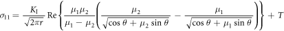

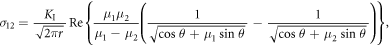
where r is the distance from the crack tip and θ is the angle measured from the axis x1 .
According to BLS results in figure 10(b), the slip traces {123} are deviated from the axis x2 = [001] by the angle β defined (see the scheme in figure B1) by a relation tg β = (a0√2)/5a0 = √2/5, i.e. β = 15.793°. In the upper part of the crystal (above x1), the angle θ (measured from the axis x1 in the anti-clockwise direction) is +θ = π/2 + β (as in figure 10(a)) and in the lower part (below x1) it is +θ = 3π/2 + β = 2π−74.207°, which corresponds to the lower slip in figure 10(c) bellow the crack plane.

Figure B1. The angle β (beta) of the slip system  in the observation plane (110)
Download figure:
Standard image High-resolution image
After summing in equation (B.1) one may write for the shear stress in the slip system $](https://content.cld.iop.org/journals/1402-4896/98/12/125974/revision2/psad0d67ieqn80.gif) (see figures 4 and 10(c) below the crack plane) following relations:
(see figures 4 and 10(c) below the crack plane) following relations:

For axial tension in a perfect crystal σ22 =  σA in the lower part and Schmid factor is
  which corresponds to 0.46, as mentioned in section 3.2. In the lower part of our cracked crystal the shear stress in the slip system
 $](https://content.cld.iop.org/journals/1402-4896/98/12/125974/revision2/psad0d67ieqn83.gif) is τb
123 = 'σ21 which means:
is τb
123 = 'σ21 which means:

where the complex variables (roots) μ1, μ2 differ for plane stress and plane strain. According to [16], for our crack orientation (001)[110] it is:
for plane stress:

and
for plane strain:

Using the roots μ1, μ2 for plane strain—see equation (B.5) and the angle θ = 2π−α, α = π/2−β = 74.207°, then according to equation (B.2), the stress components in the original system x1 = ![$[\bar{1}10],$](https://content.cld.iop.org/journals/1402-4896/98/12/125974/revision2/psad0d67ieqn84.gif) x2 = [001] and x3 = [110] are:
x2 = [001] and x3 = [110] are:

The component  follows from the relation ε33 = 0 for plane strain. Contribution from the T-stress (acting along the x1-axis) to the slip stress τb
123 is zero according to Schmid law because the direction x1 =
follows from the relation ε33 = 0 for plane strain. Contribution from the T-stress (acting along the x1-axis) to the slip stress τb
123 is zero according to Schmid law because the direction x1 = ![$[\bar{1}10]$](https://content.cld.iop.org/journals/1402-4896/98/12/125974/revision2/psad0d67ieqn86.gif) is perpendicular to the direction of the Burgers vector b = (a0/2)
is perpendicular to the direction of the Burgers vector b = (a0/2)![$[11\bar{1}].$](https://content.cld.iop.org/journals/1402-4896/98/12/125974/revision2/psad0d67ieqn87.gif)
If we consider a near distance from the crack tip r = b/2 or r = b/4 and Griffith level of loading KI = KG = 0.9115 MPa m1/2 for plane strain (see figure 12), then using equations (B.6) and (B.3) we obtain

or

with negative component in x2 = [001] direction and the positive in x3 = [110] direction. This corresponds well to the orientation of our considered Burgers vector in the ![$[11\bar{1}]$](https://content.cld.iop.org/journals/1402-4896/98/12/125974/revision2/psad0d67ieqn88.gif) direction. Magnitude (square roots) of the components correspond to 19.7 GPa for b/2 or 28.6 GPa for b/4 and they exceed the stress barrier τdisl = 16.2 GPa for dislocation emission in the
direction. Magnitude (square roots) of the components correspond to 19.7 GPa for b/2 or 28.6 GPa for b/4 and they exceed the stress barrier τdisl = 16.2 GPa for dislocation emission in the  slip system with the used potential. This means that the emissions
  observed in MD (and presented in figure 10 for the samples B50 and B60) are also possible from the point of the anisotropic linear fracture mechanics. It should be noted that in the last relations for τb
123, the required stress barrier of 16.2 GPa is exceeded even by the negative components in the x2 direction alone.
observed in MD (and presented in figure 10 for the samples B50 and B60) are also possible from the point of the anisotropic linear fracture mechanics. It should be noted that in the last relations for τb
123, the required stress barrier of 16.2 GPa is exceeded even by the negative components in the x2 direction alone.
If one considers the upper slip system $](https://content.cld.iop.org/journals/1402-4896/98/12/125974/revision2/psad0d67ieqn91.gif) in figures 10(a), (b), rotated by 180° around the fixed 'x2 = [123] axis, the signs in the matrix aij = cos('xi, xj) are changed in the first and the third row since cos(γij ± π) = −cos(γij), i.e.
in figures 10(a), (b), rotated by 180° around the fixed 'x2 = [123] axis, the signs in the matrix aij = cos('xi, xj) are changed in the first and the third row since cos(γij ± π) = −cos(γij), i.e.
and we have

For the upper slip system θ = π/2+ β, the functions in equation (B.2) are cosθ = −0.2720, sin θ = 0.9623 and the individual stress components for plane strain are
 and
and

which leads to

with the positive component in x2 = [001] direction and the negative in x3 = [110] direction, in agreement with the orientation of the Burgers vector in the upper slip system .$](https://content.cld.iop.org/journals/1402-4896/98/12/125974/revision2/psad0d67ieqn95.gif) For the distance r = b/2 and r = b/4 from the crack tip and Griffith level of loading we obtain
For the distance r = b/2 and r = b/4 from the crack tip and Griffith level of loading we obtain
 for r = b/2 and
  for r = b/4,
which is less favorable situation for the emission in comparison with the lower slip system $](https://content.cld.iop.org/journals/1402-4896/98/12/125974/revision2/psad0d67ieqn98.gif) presented above, in spite the fact that Schmid factor (0.46) for the upper and the lower slip system is the same. This 'non-Schmid behavior' can be explained in our case by the anisotropic LFM stress field at the crack tip, described by equation (B.2). Nevertheless, the magnitude (square roots of the components) τb
123 at r = b/4 corresponds to ∼17. 4 GPa, which exceeds the stress barrier τdisl = 16.2 GPa in the slip system, i.e. the emission is also possible according to the anisotropic LFM. Note that the distance b/4 corresponds to the position where the theoretical stress barrier for the slip system
presented above, in spite the fact that Schmid factor (0.46) for the upper and the lower slip system is the same. This 'non-Schmid behavior' can be explained in our case by the anisotropic LFM stress field at the crack tip, described by equation (B.2). Nevertheless, the magnitude (square roots of the components) τb
123 at r = b/4 corresponds to ∼17. 4 GPa, which exceeds the stress barrier τdisl = 16.2 GPa in the slip system, i.e. the emission is also possible according to the anisotropic LFM. Note that the distance b/4 corresponds to the position where the theoretical stress barrier for the slip system  (see figure 7 in [20]) reaches the maximum during BLS simulations in the perfect bcc iron crystal.
Declaration of competing interest
We declare that we do not have any commercial or associative interest that represents a conflict of interest in connection with the work submitted.
Conflict of interest
The authors declare that they have no conflict of interest.