
Abstract
Measurements had been performed of strong electromagnetic pulses (EMPs) generated as a result of laser–target interaction at the sub-ns kJ-class Prague Asterix Laser System facility. Two conductive Prodyn FD5C D-dot pencil probes were used. Measurements were performed inside the experimental chamber and outside the chamber in a large chamber window 40 cm in diameter in a setup that guaranteed 6 GHz bandwidth. A very good signal-to-noise ratio (17:1) was obtained after some steps were taken to ensure proper EMP shielding of the data collection setup. The EMP signal in the time domain was found to have the form of a sharp initial spike followed by gradually decaying oscillations interspersed with some secondary spikes. The values of the vertical component of the electric field strength were estimated. The highest value recorded in this experiment was  kV m−1 at a distance of 40 cm from the target. It was observed that plastic targets—particularly the 100s of µm thick plastic foils—tend to generate stronger EMP fields than Cu and Au targets. A time-frequency analysis was performed for a typical shot, clearly showing some spectral features that appear only sometime after the start of the signal and hence indicate EMP generation from secondary sources. Electrons ejected from the target were recorded with the energies exceeding 1.5 MeV, which indicates that highly energetic processes are triggered as a result of the laser–target interaction.
Export citation and abstract BibTeX RIS

Original content from this work may be used under the terms of the Creative Commons Attribution 4.0 license. Any further distribution of this work must maintain attribution to the author(s) and the title of the work, journal citation and DOI.
1. Introduction
The laser–target interaction at high-power laser facilities is often accompanied by the emission of strong electromagnetic pulses (EMPs) with frequencies in the range from tens of MHz to several GHz. Such pulses may affect electronic equipment involved in data acquisition or used for target and diagnostics manipulation, greatly complicating in this way realization of laser–plasma experiments, particularly at petawatt power and megajoule energy laser facilities [1–10]. For this reason the problem of a proper characterization of the laser-generated EMP for various laser and target conditions, a precise identification of the sources of EMP and studies aimed at the EMP mitigation received considerable attention, as had been thoroughly reviewed in [11], with figure 75 in this reference giving a good overview of the EMP values measured so far at various laser facilities. In particular, the target neutralization current resulting from laser-induced electric polarization of the target was identified as an important source of EMP [12–14]. The EMP problem continues to attract interest and new results on EMP measurements are continually being published, both for the short-pulse [15–18] and long-pulse facilities [19]. It should be noted that mechanisms involved in EMP generation are relevant also to other areas of laser plasma research, such as the post-acceleration guiding of laser-accelerated ions [20, 21] and generation of strong quasi-static magnetic fields with the use of capacitor-coil targets [22–25].
In this note we report on the EMP measurements performed at Prague Asterix Laser System (PALS) facility [26]. The PALS laser delivers ∼300 ps pulses at  μm fundamental wavelength, with energies on the order of kJ, achieving ∼1016 W cm−2 laser intensities. The EMP studies at PALS are of considerable interest for at least two reasons. Firstly, the pulse duration and the beam intensity of this laser are directly relevant to the shock ignition (SI) mechanism in the inertial confinement fusion, and indeed a number of studies of shock-ignition laser–plasma physics had been realized at this facility [27–31]. Secondly, with the laser irradiance parameter
  W μm2 cm−2 this facility operates above the threshold for various plasma instabilities such as the stimulated Raman scattering (SRS) and the two-plasmon decay (TPD) [32–34]. Such instabilities are known to be potentially prolific sources of hot electrons which are the primary cause of the EMP effects. Indeed, PALS was notorious for high EMP levels. The EMP amplitudes at PALS were measured in a variety of experimental arrangements [13, 35–42] using loop probes, monopole antenna, a planar super-wideband antenna and a horn antenna. These measurements provided valuable qualitative insight into the EMP characteristics at PALS laser parameters. However, in neither of these measurements the amplitudes and spectra were adjusted for the response characteristics of the probes that were used. Furthermore, a very poor signal-to-noise ratio of 5:1 or less was reported in [41] and doubts were expressed regarding the general usefulness of the conductive probes in measurements of laser-induced EMP. The aim of our experiment was to complement previous investigations by performing a measurement with the use of a high-bandwidth D-dot probe. Our intent was to reexamine the issue of the signal-to-noise ratio and clarify the usefulness of conductive electromagnetic probes for measurements of laser-generated EMP and—if possible—obtain a direct estimate of the EMP electric field strengths.
We used two Prodyn FD5C D-dot probes (nominally 50 GHz bandwidth) connected via high-quality concentric cables to a 6 GHz bandwidth oscilloscope to collect the signal. Measurements were performed inside the experimental chamber and outside the chamber in a chamber window. Both thin and thick plastic and metal targets were used. We found that a very good signal-to-noise ratio may be achieved with the FD5C probes, provided some rules are observed. We also found that with a higher bandwidth the overall picture of the EMP signal is qualitatively changed, becoming similar to that observed at short pulse facilities. On the basis of these measurements we are able to provide an estimate of the absolute value of the EMP electric field strength inside and outside the chamber and compute the corresponding spectra. The wideband characteristics of the signal we record raise some questions regarding the origin of this signal.
The paper is organized as follows: in section 2 we describe the experimental setup, in section 3 we report on EMP measurements made outside of the experimental chamber in the chamber window, in section 4 we report on EMP measurements made inside the experimental chamber. In section 5 we describe the efforts we made and procedures we implemented to ensure the high signal-to-noise ratio in our EMP measurements. The proposed ways to resolve this technical issue will benefit many other groups interested in laser-generated EMP studies. In section 6 we present measurements of electrons ejected from the target, in which electron energies exceeding 1.5 MeV were recorded. Section 7 is devoted to the measurement of the target neutralization current, section 8 contains discussion of the results, where we confront EMP measurements with neutralization current measurements, and in section 9 we give a summary.
2. Experimental setup
The PALS laser facility is an iodine laser system [26]. The full width at half maximum (FWHM) pulse duration in our experiment was 290 ± 20 ps, and the laser pulse energy on target EL
—excluding few shots in which it was deliberately reduced—was 590 ± 30 J. The beam power was monitored online for every shot; in figure 1 we show the normalized temporal beam intensity profiles for several representative shots. The temporal contrast on a multi-ns scale was on the order of  . The laser beam 290 mm in diameter was directed onto the target at normal incidence and focused by a lens of 600 mm focal length to a spot 70 μm in diameter at FWHM. (The size of the laser spot was estimated on the basis of interferometric and x-ray images obtained in previous experiments. The laser intensity distribution in the laser spot obtained in the case when the phase plate is used was found to be Gaussian with FWHM diameter 100 μm [43]. In our experiment the phase plate was not used, which allowed for a smaller focal spot, albeit with possibly a less regular intensity distribution.) Assuming Gaussian distribution in space and time this implies average intensity
  W cm−2 and average value of the irradiance parameter
  on the order of
  W μm2 cm−2. The targets were CH2 foils with thickness 0.125 mm, 0.200 mm and 0.5 mm, CD2 foils with thickness 0.5 mm and 1.0 mm, Au foil 0.06 mm, and Cu foil 0.05 mm, which were pasted on a Al target holder 63 mm long, 15 mm wide and 5 mm thick. A massive Cu target in the form of a slab 50 mm long, 5 mm wide and 5 mm thick was also used. The target holder and the massive Cu target were mounted vertically. All shots were performed in a 10−5 mbar vacuum.

Figure 1. The temporal laser pulse profile for some representative shots in this experiment, normalized to the maximum intensity.
Download figure:
Standard image High-resolution imageA schematic view of the experimental setup is shown in figure 2, where the chamber (X, Y, Z) coordinate system is also indicated, with (0, 0, 0) point corresponding to the laser–target interaction point. The PALS experimental chamber is approximately a sphere 1 m in diameter. EMP measurements were performed using two Prodyn FD5C D-dot probes which were mounted on dielectric supports inside the experimental chamber, as well as outside of the chamber, in a large window 40 cm in diameter, made of 3 cm thick BK7 glass. The signal collected by the probes was recorded using a Tektronix TDS 6604 oscilloscope with 6 GHz bandwidth and maximally 20 GS s−1 sampling rate (50 ps sampling interval) on two channels, placed in a Faraday cabinet for protection against electromagnetic interference. The probes were connected to the oscilloscope by high-quality double-shielded SubMiniature version A (SMA) Totoku TCF500 concentric cables, certified for frequencies up to 18 GHz, passing through a concentric vacuum feedthrough with floating shield, placed in the chamber wall, and through a concentric feedthrough with a grounded shield in the Faraday cabinet well (1.5 m inside the chamber, 2.5 m between the chamber and the Faraday cabinet and 1.0 m inside the cabinet). The cable sections inside the chamber and between the chamber and the Faraday cabinet were covered with an additional external braided shield for added protection against parasitic interference. There was no electrical connection between the braided shield and the external conductor of the coaxial cable inside the shield; for cables inside the experimental chamber the braided shields were grounded inside the chamber to the chamber wall, and shields of the external cables were not grounded at all. Additional concentric attenuators were mounted on the oscilloscope terminals: typically 26 dB for measurements inside the chamber and 10 dB for measurements outside of the chamber. The oscilloscope was enclosed in a Faraday cabinet which was put on autonomous battery power supply for the shots. Prior to the actual EMP measurements a number of shots were devoted to improve the signal-to-noise ratio, with the final result being 17:1 for properly chosen signal attenuation at the oscilloscope terminal. These efforts are described in detail in section 5. All EMP measurements reported in sections 3 and 4 were then made in this optimized low-noise setting.
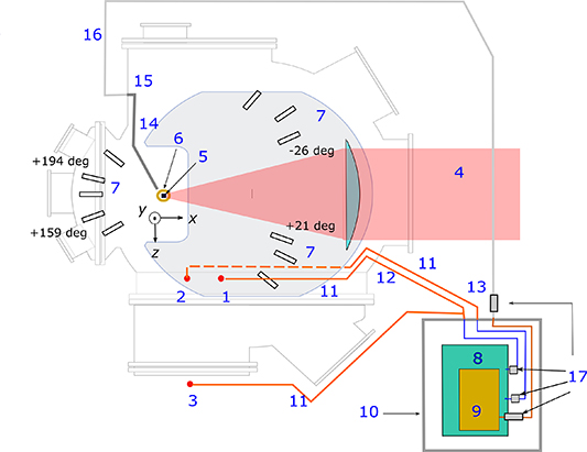
Figure 2. A schematical top view of the experimental setup: (1) FD5C D-dot probe in position 1; (2) FD5C D-dot probe in position 2; (3) FD5C D-dot probe in position 3, outside the chamber; (4) laser beam; (5) target; (6) inductive target return current probe; (7) permanent magnet spectrometers; (8) Tektronix TDS 6604 oscilloscope (6 GHz); (9) Tektronix TDS 694C oscilloscope (3 GHz); (10) Faraday cabinet; (11) high-quality double-shielded SMA concentric cables with additional external copper braided shield; (12) vacuum concentric SMA feedthrough with a floating shield; (13) concentric feedthroughs with grounded shield; (14) concentric cable with additional external braided shield; (15) concentric vacuum feedthrough with grounded shield; (16) double-shielded concentric cable; (17) signal attenuators. The X, Y, Z chamber reference frame is also indicated, with the origin at the laser–target interaction point.
Download figure:
Standard image High-resolution imageThe Prodyn FD5C probes are pencil-sized probes that provide a single unbalanced output. According to the specification, the 3 dB point of these probes is above 50 GHz. The signal  of these probes depends linearly on the derivative of the electric displacement vector component parallel to the axis of the probe,
  , where in vacuum
  , with
  being the electric permittivity of the vacuum. The exact relation is best expressed in terms of the Fourier transforms (our conventions for the discrete and continuum Fourier transforms are summarized in appendix
where  is the resistance of the probe and
  is the frequency-dependent equivalent area of the probe. The expression we use for
  is described in appendix
  vector is oriented from the active tip of the probe to the SMA connector. Probes were mounted on custom dielectric supports to minimize parasitic interference. In all measurements reported in this paper the probes were oriented vertically, i.e. they were sensitive to the Y-component of the electric field strength. The reason for choosing this orientation is that in the preferred scenario where the dominant source of EMP is the target neutralization current this component is expected to be dominant.
Apart from the electric field strength, also the target neutralization current was monitored, using an inductive probe being an evolution of the design presented in [13]. The mutual inductance parameter that characterizes this type of probe [13] was 0.59 nH. (In fact the setup consisted of two probes of such type mounted together, with the aim to obtain a balanced output, but effectively only one of them gave useful signal.) The signal collected by the probe was recorded using a Tektronix 694C oscilloscope with 3 GHz bandwidth and 10 GS s−1 sampling rate (100 ps sampling interval) with the signal interpolation turned on. The oscilloscope was placed in a Faraday cabinet. The probe was connected to the oscilloscope via 0.8 m RG-58 concentric cable (protected inside the chamber by an additional external braided shield grounded to the chamber wall) passing through a concentric vacuum feedthrough with a grounded shield, followed by 4.0 m RG-214 double-shielded concentric cable connected to a grounded shield feedthrough in the Faraday cabinet and finally inside the cabinet 2.0 m RG-316 concentric cable connecting to the oscilloscope. A 60 dB attenuation was applied at the entrance to the Faraday cabinet and a smaller attenuation at the oscilloscope terminal.
Finally, permanent-magnet electron spectrometers were used to monitor electrons escaping from the target. The spectrometers were custom 20 mm × 95 mm × 95 mm assemblies containing a permanent magnet placed between magnetically soft steel plates that maintained practically homogenous magnetic field of 95 mT perpendicular to the direction of the incoming electrons [45]. Electrons were entering the spectrometer through a circular aperture 1 mm in diameter. Deflected electrons were recorded with the use of Fujifilm BAS-SR imaging plates oriented parallel to the line of sight of the spectrometer to reduce the noise. Lead screening plates were used to limit the effect of energetic photons. Spectrometers were capable of recording electrons in the energy range from 50 keV to 1.5 MeV. They were positioned inside the experimental chamber at angles −45°, −36°, −26°, +21°, +28°, +45°, +148°, +159°, +180°, +194°, +220°, and distances varying from 14 cm to 46 cm, as indicated in figure 2, with the input aperture at the level of the laser beam.
3. EMP measurements performed in the chamber window
Let us start our analysis with the discussion of the data taken outside the experimental chamber in the chamber window. The probe setup in this measurement is shown in figure 3. The importance of this measurement is that it is sensitive to the signal that propagates into the experimental hall and directly affects scientific instruments placed there. Secondly, the output of the FD5C probes in this arrangement is unlikely to be affected by a direct interaction with charged particles emitted from the target of plasma outflows, since the probes are screened from any particles emitted by the target by a 3 cm thick BK7 glass. On the other hand, the disadvantage of this arrangement is that probes are sensitive to the EMP signal that may not originate directly from the chamber window, but may be the signal bouncing off the walls of the experimental hall. Furthermore, we should be aware that the window distorts the spectrum of the recorded signal since it attenuates low frequencies (the wavelength on the order of the window diameter 0.4 m corresponds to the frequency of 750 MHz). The FD5C probes were placed at a distance of 12 cm from the window. They were oriented vertically in antiparallel way with the active tips separated by 2 cm, so that in an ideal case the oscilloscope signals produced by the probes would be of equal magnitude and opposite sign, which provides a good cross-check on the validity of the measurement.
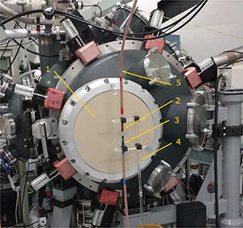
Figure 3. The setup for the EMP measurement outside of the target chamber, in the chamber window: (1) 3 cm thick BK7 glass window 40 cm in diameter, protected by a cardboard lid; (2) FD5C D-dot probe pointing vertically downwards; (3) FD5C D-dot probe pointing vertically upwards; (4) dielectric support; (5) double-shielded concentric cable with additional external braided shield.
Download figure:
Standard image High-resolution imageA typical signal recorded in the chamber window by the probe pointing upwards is shown in figure 4 (#52 065—0.06 mm Au target, EL = 609 J). This picture is familiar from many EMP measurements [6, 7, 46], with a step-like signal growth at the beginning, followed by a gradual decay. The whole signal lasted approximately 100 ns. The signal was filtered using a low-pass parabolic filter with 6 GHz pass frequency to eliminate spurious high-frequency content.
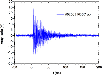
Figure 4. Example of a raw signal recorded in the chamber window by the FD5C probe pointing upwards, as a function of time, for a shot on a 0.06 mm Au target with EL = 609 J (#52 065), filtered with a 6 GHz parabolic low-pass filter.
Download figure:
Standard image High-resolution imageThe vertical component of the electric field strength Ey
was computed from the FD5C probe signal by performing the following operations: (a) include a sign factor to account for the orientation of the probe and calculate the discrete Fourier transform (DFT) of the signal; (b) correct the signal for the frequency-dependent attenuation of the concentric cables connecting probe to the oscilloscope; (c) insert the frequency-dependent equivalent area of the FD5C probe according to the formulas given in [44]; (d) perform the inverse discrete Fourier transform and obtain  , assuming vacuum relation between
  and
and  ; (e) perform numerical integration to obtain Ey
(t). The latter step requires some care in the treatment of the low-frequency component of the signal, which we explain further below. The result for Ey
(t) corresponding to the signal shown in figure 4 is displayed in figure 5. It should be noted that this result is subject to uncertainty arising from the uncertainty in the determination of the equivalent area Aeq of the probe. The uncertainty of Ey
(t) is estimated in section 4. The signal in figure 5 shows a slight enhancement above the level of oscilloscope noise few ns before the onset of strong EMP, which we attribute to the EMP signal seeping out into the chamber and directly affecting the oscilloscope readings in a slight way, as discussed in section 5.
; (e) perform numerical integration to obtain Ey
(t). The latter step requires some care in the treatment of the low-frequency component of the signal, which we explain further below. The result for Ey
(t) corresponding to the signal shown in figure 4 is displayed in figure 5. It should be noted that this result is subject to uncertainty arising from the uncertainty in the determination of the equivalent area Aeq of the probe. The uncertainty of Ey
(t) is estimated in section 4. The signal in figure 5 shows a slight enhancement above the level of oscilloscope noise few ns before the onset of strong EMP, which we attribute to the EMP signal seeping out into the chamber and directly affecting the oscilloscope readings in a slight way, as discussed in section 5.

Figure 5. The vertical component of the electric field strength vector measured in the chamber window, as a function of time, corresponding to the FD5C signal shown in figure 4. A high-pass filter with the pass frequency of 50 MHz was applied so that the null signal region preceding the spike was reproduced in a satisfactory way.
Download figure:
Standard image High-resolution imageIn figure 6 we show the same function on a finer time scale. We see that the EMP signal starts rapidly with a narrow initial spike followed by a number of secondary spikes, some of them larger in magnitude than the initial spike. The field values extracted from the data collected by the FD5C probe pointing upwards are compared to the field values based on data collected by the FD5C probe pointing downwards. After inverting the sign of the signal of the probe pointing upwards to account for the orientation of the probe the results should be similar. As we may see, this is indeed the case: the agreement between the two curves is quite remarkable, which provides a very strong argument supporting validity of our measurements. Additionally, individual data points from the oscilloscope record for the probe pointing upwards are displayed to illustrate the signal sampling (the sampling interval was 50 ps).
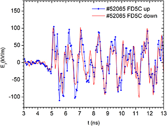
Figure 6. The vertical component of the electric field strength vector recorded in a shot on 0.06 mm Au target with EL = 609 J (#52 065), shown on a fine time scale. The result from the probe pointing upwards (thick blue line with dots) is compared to the result from the probe pointing downwards (thin red line line). Individual data points from the oscilloscope record are displayed to illustrate the signal sampling.
Download figure:
Standard image High-resolution imageWhile performing the numerical integration of the data for dEy /dt we encounter the problem of contribution from low-frequency region of the spectrum. Such contributions may correspond to a low signal level, but contribute strongly to the result for the field values when they persist over a longer period of time. In general, large low-frequency contributions to EMP may arise as a result of a number of physical processes, such as: (a) low-frequency contribution to the target neutralization current [40, 41]; (b) currents generated by charged particles striking the chamber walls [2, 8]; (c) currents flowing in the plasma filling the chamber [47]. The low-frequency contributions may also arise from wakefields created behind the obstacles by flows of plasma ejected from the target [48]. Furthermore, a direct interaction of the probe with the plasma ejected from the target, unrelated to any electromagnetic emission, may also result in a probe response similar to the low-frequency EMP signal. However, in the case of measurements performed outside of the experimental chamber these processes cannot contribute or are strongly suppressed; in particular, the 40 cm diameter window should act as a high-pass filter with pass frequency approximately 750 MHz. This means that there should be no problem in integrating the data collected in the window.
There remains one more obstacle, related to the fact that any oscilloscope measurement is contaminated by the unavoidable electronic noise generated by the oscilloscope hardware. The oscilloscope noise is a white noise, i.e. it provides a nonzero frequency-independent contribution to the overall signal spectrum. This makes the DFT spectrum to behave for small f as a constant, instead of at least  , as one would expect for a Fourier transform of a quantity that is a time derivative of a transient signal. Upon integration, which essentially amounts to multiplication of the Fourier transform by a factor of
  , the terms in DFT corresponding to lowest frequencies are strongly enhanced. This is illustrated in figure 7, where the spectrum of the Ey
(t) signal presented in figure 5 is compared to the spectrum of a 200 ns stretch of the null part of the signal that precedes the onset of strong EMP, processed in the same way as the genuine EMP signal. (We use a DFT normalization in which the DFT spectrum values are to a good approximation equal to the discretization of the continuum Fourier transform of the physical signal, as is explained in appendix
, the terms in DFT corresponding to lowest frequencies are strongly enhanced. This is illustrated in figure 7, where the spectrum of the Ey
(t) signal presented in figure 5 is compared to the spectrum of a 200 ns stretch of the null part of the signal that precedes the onset of strong EMP, processed in the same way as the genuine EMP signal. (We use a DFT normalization in which the DFT spectrum values are to a good approximation equal to the discretization of the continuum Fourier transform of the physical signal, as is explained in appendix  enhancement in the DFT of the signal manifests itself in the appearance of large-amplitude low-frequency oscillations in time domain. One may cope with this effect by applying a high-pass filter to the signal being processed, with the pass frequency chosen according to circumstances, as had been pointed out in [49]. A simple criterion that may be applied is to adjust the pass frequency so that in the region before the onset of strong EMP, where we do not expect to have signal, the result of integration is indeed reasonably close to zero. For this reason it is important to keep the external attenuation as small as possible when collecting the data, to ensure largest possible ratio of the signal to the oscilloscope noise (which is not easy, because the level of the electromagnetic signal fluctuates strongly from shot to shot, so when we apply attenuation which is too small this may easily result in the loss of data due to oscilloscope saturation or even damage to the oscilloscope). In the case of the EMP measurements performed in the chamber window we found that using 50 MHz pass frequency was sufficient to fulfill this criterion. The larger the electronic noise, the higher filter cutoff frequency has to be chosen. The downside of the high-pass filtering is that we loose any physical signal that might be present below the pass frequency, but in the case of measurements in the chamber window such contributions are unlikely.
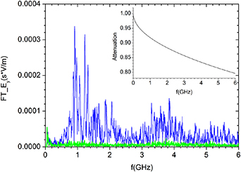
Figure 7. Blue line—the Fourier spectrum of the electric field strength evolution shown in figure 5 (#52 065); green line—the Fourier spectrum of the oscilloscope noise; inset—the signal attenuation factor in the concentric cables connecting probes to the oscilloscope in this measurement.
Download figure:
Standard image High-resolution imageAs seen from figure 7, the Fourier spectrum of the Ey (t) signal presented in figure 6 is essentially contained between 0.5 GHz and 2.4 GHz, with a pronounced peak near 0.8–1.0 GHz and 1.2–1.4 GHz, as well as a broad feature extending from 3.2 to 4.5 GHz. Additionally, the attenuation factor for the signal transferred by the coaxial cables of the probes in this measurement is shown in the inset.
4. EMP measurements performed inside the experimental chamber
Measurements of the EMP signal inside the experimental chamber were performed using the setup shown in figure 8, where two FD5C probes were mounted vertically on dielectric supports in antiparallel way, with active tips separated by 2 cm. The tip of the probe pointing upwards was located at X = 17 cm, Y = 0 cm, Z = 29 cm in the target chamber reference frame; it was on the same level above the breadboard as the laser beam.
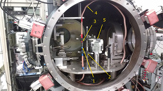
Figure 8. The setup for EMP measurement inside the experimental chamber: (1) FD5C D-dot probe pointing upwards; (2) dielectric support; (3) FD5C D-dot probe pointing downwards; (4) double-shielded concentric cable with additional external braided shield; (5) permanent magnet electron spectrometers.
Download figure:
Standard image High-resolution imageA characteristic feature of measurements performed with FD5C probes inside the chamber is that probe response shows a pronounced low-frequency dependence, as illustrated in figure 9 for a shot on 0.5 mm CH2 target with pulse energy 583 J on target (#52 059). (The signal was filtered using a low-pass parabolic filter with 6 GHz pass frequency to eliminate spurious high-frequency content.) In this figure the signal from the probe pointing down is compared to the signal from the probe pointing up, multiplied by  to account for opposite orientation. If the low-frequency features were of electromagnetic origin, the signals should overlap, but this is not the case. We attribute the long-timescale evolution of the signal to direct interaction of the probes with the plasma ejected from the target, on the basis of observation from our further experience with these probes which showed that the effect disappears when a Teflon screen is placed across the line of sight between the probes and the target. The low-frequency features complicate data processing, as they tend to dominate the signal integration required to obtain the field strength evolution. We resolved this issue by applying a high-pass filter; we found that a filter with 150 MHz stop frequency was sufficient to obtain stable integration results in all shots in this experiment where measurement was performed inside the experimental chamber. This means, however, that our analysis is insensitive to any possible genuine low-frequency EMP signals below 150 MHz [41]. This is not a problem for our experiment, since our primary goal in this experiment was to explore the high-frequency content of the EMP spectrum. A dedicated study with a different set of probes and a different data-collection strategy would be required to characterize any EMP effects in the low-frequency range.

Figure 9. The raw signal captured by the FD5C probe pointing downwards (red line) compared to the signal captured by the FD5C probe pointing upwards (blue line) multiplied by (−1) to account for the orientation of the probe, for a shot on a 0.5 mm CH2 target with EL = 583 J (#52 059). A 6 GHz parabolic low-pass filter was applied.
Download figure:
Standard image High-resolution imageThe evolution of the vertical component of the EMP electric field strength on a large time-scale has the form similar to that shown in figure 5, and on a shorter time-scale it is shown in figure 10. As a cross-check we compare the result extracted from the signal taken by the FD5C probe pointing up with the average of the field values obtained from both of the probes. A very good agreement is found, which makes us confident about the validity of our measurement.

Figure 10. The vertical component of the EMP electric field strength vector at the probe location, as obtained from the FD5C probe pointing upwards (solid line), compared to the average value of the electric field strength from the probe pointing upwards and probe pointing downwards (dash-dotted line), for a shot on a 0.5 mm CH2 target with EL = 583 J (#52 059). A 150 MHz high-pass filter had been applied.
Download figure:
Standard image High-resolution imageThe electric field strength values we extract are subject to uncertainty arising from uncertainty in the equivalent area Aeq of the FD5C probe. As discussed in [44], the equivalent area of the FD5C probe is frequency-dependent and below 1 GHz it deviates substantially from the datasheet value; the relevant formula is given in appendix
In figure 11 we show the Fourier spectrum of the electric field strength evolution shown in figure 10. Apart from the overall normalization resulting from higher field values this spectrum is similar to the spectrum displayed in figure 7 for the measurement performed in the chamber window in that the bulk of the spectrum is contained in the region between 0.5 GHz and 2.4 GHz and a broad bump centered at 3.6 GHz. The difference is that in addition we see a pronounced narrow spike near 0.80 GHz, a spike near 1.36 GHz, and a broad feature lying between 1.48 GHz and 1.72 GHz.
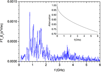
Figure 11. The Fourier spectrum of the vertical component of the electric field strength vector extracted from the signal collected by the FD5C probe pointing upwards, for a shot on a 0.5 mm CH2 target with EL = 583 J (#52 059). Inset—the signal attenuation factor introduced by the concentric cables connecting probes to the oscilloscope in this measurement.
Download figure:
Standard image High-resolution imageMore insight into the nature of the various peaks in the spectrum could be obtained by inspecting the short-time Fourier transform for this shot, shown in figure 12. A 256-point Hamming window (covering 12.8 ns at 50 ps sampling interval) was used to construct this contour plot, with 224 points overlap. The time scale is shifted so that the intensity of a pixel represents the magnitude of the contribution to the spectrum in the given frequency bin evaluated for a time interval centered at this pixel. The frequency binning is 78 MHz. Interestingly, we see that at the start of the signal there are strong contributions only at frequencies near the 1.0 GHz, 1.6 GHz and 2.1 GHz. Moving further along the time axis, after approximately 10 ns from the start of the signal we begin to see enhancement near 0.8 GHz, which is represented in the overall spectrum by a prominent narrow spike in figure 11. It is hence tempting to associate this spike with some sort of electromagnetic resonance excitation inside the chamber, although it is not easy to identify the relevant eigenmode (the lowest eigenfrequency of the PALS chamber with the metallic target holder, the focusing lens and the glass window taken into account was found to be 287 MHz [38]). Furthermore, we see that the bump in the spectrum near 3.6 GHz is also an effect delayed in time, appearing approximately 10 ns after the start of the signal. A possible explanation might be that it originates from the interaction of the expanding plasma with fine elements inside the chamber [50] or from a resonant rescattering of the primary EMP impulse by such elements.
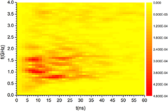
Figure 12. A contour plot of a short-time Fourier transform of the electric field strength for a shot on a 0.5 mm CH2 target with EL = 583 J (#52 059). A 256 point Hamming window was used with 224 points overlap. The time scale is shifted so that the intensity of a pixel represents the magnitude of the contribution of the given frequency bin to the spectrum evaluated in a time interval centered at this pixel. There are no discernible features on this plot above 4 GHz.
Download figure:
Standard image High-resolution imageFinally, in figure 13 we present a summary of the extremal electric field strength values recorded inside the chamber for different targets and different laser pulse energies. Extremal values were obtained using the average of signals from the two FD5C probes. Most of the data points are clustered in the energy range between 570 J and 630 J. In figure 14 we show the extremal field values using a finer energy scale; in this figure also the data points from measurements performed in the chamber window are included. The scatter of the results for different targets is rather large, but some trends may be identified. The highest extremal value was obtained in this experiment with the thinnest (0.125 mm) CH2 target, giving 620 kV m−1, with the asymmetric uncertainty from the FD5C probe calibration of  kV m−1 and
  kV m−1. Additionally, for this target type data points were obtained for energies extending down to 301 J and the extremal field values seem to decrease in a manner consistent with what had been observed on other laser systems [6, 14, 46, 51]. We may also say that CH2 and CD2 targets generated in general stronger EMP than thin foil Cu targets. Naturally, the extremal field values recorded in the chamber window—available in this study only for metal targets—are lower than values measured for metal targets inside the chamber. Such difference in amplitudes is expected because of the fact that the 40 cm diameter chamber window provides a smooth cutoff on frequencies below 750 MHz, as was mentioned in section 3. Another factor that could affect this difference is the contribution of the eigenmodes. Eigenmode excitation in the PALS chamber was studied in [38]. The fundamental frequency was found to be 287 MHz. Fields related to eigenmodes do not propagate outside the chamber as easily as the reverberating signal. The highest value recorded outside the chamber in the chamber window was obtained in a 615 J shot on 0.06 mm Au target:
  kV m−1.

Figure 13. The extremal values of the vertical electric field strength component recorded by the FD5C probes inside the chamber, obtained from the average of the two probe readings, as a function of the laser energy on target, for various targets. It appears that the EMP generated off plastic targets is in general substantially stronger than EMP off thin metal targets.
Download figure:
Standard image High-resolution image
Figure 14. The extremal values of the vertical electric field strength component recorded for laser energies in vicinity of 600 J, for various targets. Results from measurements performed in the chamber window are indicated with open symbols.
Download figure:
Standard image High-resolution image5. The problem of the signal-to-noise ratio
An important issue that has to be resolved in EMP measurements is the problem of the signal-to-noise ratio, i.e. the ratio of the signal collected by the probe to the magnitude of electromagnetic disturbances picked up by the connecting cables, feedthroughs, or even by the oscilloscope itself. In previous experiments at PALS it was observed that the signal-to-noise ratio in EMP measurements is quite poor [41], to the extent that the very usefulness of the conductive probes for measurements of laser-generated EMP was put in doubt. (In [41] it was suggested that using a delay line consisting of 70 m or more of a cable might allow to separate signal from the noise, but this would work only up to 500 MHz or so due to the fact that long cable acts as a low-pass filter.) Therefore it was our primary concern to figure out what is the cause of this behavior and investigate how the signal-to-noise ratio may be improved. To this end prior to the measurements reported in sections 3 and 4 we made a series of measurements with two FD5C probes mounted in a similar way, while one of them was blinded to electromagnetic signals by wrapping it in aluminum foil, as shown in figure 15. Both probes were mounted pointing vertically upwards, with the position of the tip of the shielded probe at X =5 cm, Y = 12 cm, Z = 29 cm in the coordinate system defined in figure 2, and the tip of the unshielded probe at X = 17 cm, Y = 12 cm, Z = 29 cm. The wrapping foil was electrically connected to the external braided shielding of the cable, which in turn was grounded inside the chamber to the chamber wall. The braided shield was insulated from the outer shield of the cable and the SMA probe connector.
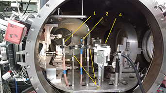
Figure 15. The setup for testing signal-to-noise ratio in the EMP measurements using the FD5C D-dot probes: (1) shielded FD5C D-dot probe pointing upwards; (2) unshielded FD5C D-dot probe pointing upwards; (3) dielectric supports; (4) permanent magnet electron spectrometers.
Download figure:
Standard image High-resolution imageAt first the signal attributed to the probe wrapped in the aluminum foil was rather large compared to the signal from the unshielded probe, as is shown in figure 16. However, the maximum of the parasitic signal was delayed relative to the maximum signal from the unshielded probe that was placed close to the shielded probe. This suggested that the parasitic signal was not due to the original EMP being improperly resolved by the D-dot probe, but was picked up somewhere along the signal path from the probe to the oscilloscope. Through a painstaking step-by-step analysis we found that the signal recorded by the oscilloscope as noise was in fact due to the EMP leaking out of the experimental chamber through the laser input window and being directly picked up by the oscilloscope electronics, despite the fact that oscilloscope was housed in a Faraday cabinet. We found that in order to reduce the parasitic signal the following steps were necessary: (a) all apertures in the Faraday cabinet had to be sealed (in the electromagnetic sense), in particular, the ventilation hole that was covered with only a thin wire mesh had to be nearly totally obstructed by a metal plate (this created the risk of overheating the oscilloscopes, so the Faraday cabinet had to be closed just before the shot and opened immediately after the shot); (b) the signal must be brought into the Faraday cabinet only via dedicated feedthroughs; (c) large signals being brought into the Faraday cabinet—such as the signal from the return current probe, which was also monitored in this experiment—should be avoided by applying attenuation at the feedthrough, not at the oscilloscope terminal; (d) the main power supply has to be disconnected before the shot and oscilloscopes inside the cabinet switched to battery power.
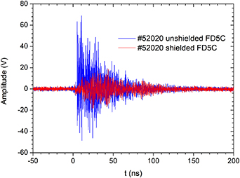
Figure 16. The probe signal from the FD5C probe shielded with Al foil, compared to the signal from the unshielded FD5C probe placed nearby, illustrating poor signal-to-noise ratio with the initial setup, for a shot on a CH2 target with EL = 497 J (#52 020). A low-pass parabolic filter with 6 GHz pass frequency was applied.
Download figure:
Standard image High-resolution imageAnother important factor was that both inside and outside the chamber we used for the FD5C probes high-quality double-shielded concentric cables (i.e. with the outer conductor consisting of two layers) which provide excellent shielding of the inner conductor carrying the signal, while in some of the previous investigation at PALS the RG58 single-shielded cable was used. With all these precautions a significant improvement in the signal-to-noise ratio in the time domain was achieved, as shown in figure 17. (A low-pass parabolic filter with 6 GHz pass and 7 GHz stop frequency was applied to the signal to remove the spurious high-frequency content.) The fact that the signal from the shielded probe is practically on the level of oscilloscope noise is a proof that data recorded by the FD5C probe inside the chamber are not contaminated by parasitic fluctuations in any significant way, despite the harsh electromagnetic environment. Taking a closer look at figure 17 we do nevertheless notice a slight increase in the signal noise starting few ns before the main spike. Our interpretation is that this is due to the main EMP signal which propagates out of the experimental chamber through the laser input window and despite all our precautions directly affects the oscilloscope, traveling in a shorter time than the signal propagating in the coaxial cables at 0.7 of the speed of light in vacuum. However, with the magnitude of the first large spike in the signal from the unshielded probe being 80.4 V, the maximum magnitude of the signal preceding the first spike by more than 350 ps being 4.7 V and the overall maximum magnitude of the signal in the channel of the shielded probe being 4.2 V, we obtain the overall the signal-to-noise ratio better than 17:1. The same good signal-to-noise ratio was confirmed in a separate shot for the measurements taken outside the chamber in the chamber window. All measurements reported in sections 3 and 4 were performed with the use of this optimized setup.

Figure 17. The raw signal from the FD5C probe shielded with Al foil compared to the signal from the unshielded FD5C probe placed nearby, illustrating excellent signal-to-noise ratio achieved after data collection was optimized to suppress parasitic signals, for a shot on a 1 mm CD2 foil with EL = 606 J (#52 035). A low-pass parabolic filter with 6 GHz pass frequency was applied.
Download figure:
Standard image High-resolution imageOne may ask whether the signal-to-noise ratio could be improved by simply subtracting the signal obtained with the shielded probe from the signal obtained with the unshielded probe. This is certainly possible, but one would have to use two identical probes located very close to each other, with identical electrical paths, and use two oscilloscope channels to measure a single observable. Furthermore, such subtraction makes sense only when the shielded probe signal is in reasonable proportion to the unshielded probe signal. Hence signal-to-noise reduction procedures described above would have to be applied anyway.
6. Characterization of electrons ejected from the target
A primary cause of the EMP emission in laser–target interactions is the effect of hot electron generation, hence it is useful to complement the EMP measurements with some data on the hot electrons. In this experiment we collected data on electrons ejected from the target using 11 permanent-magnet spectrometers distributed in the experimental chamber in the same plane at some distance from the target to cover all four quadrants relative to the laser axis. It is found that the distribution of electrons is with a good approximation symmetric with respect to the laser axis, but it depends strongly on the viewing angle relative to the target normal. On the back of the target the distribution function for electrons ejected along the target normal—i.e. at 180° viewing angle—lies visibly below the distributions for electrons ejected at small angle relative to the target normal, i.e. at viewing angles +159° and +194°, and the distribution functions rapidly fall off for large viewing angles. On the front side of the target observation of hot electrons along the target normal was not performed; the electron distribution functions were found to achieve highest values at the smallest available angles relative to the front target normal, i.e. at −26° and +21°, and to rapidly fall off at larger angles.
In figure 18 we show the ejected electron energy spectra recorded at the selected viewing angles +21° and +194° for the following shots: #52 059 (target 0.5 mm CH2, EL = 583 J, max|Ey
| = 460 kV m−1), #52 036 (target 1 mm CD2, EL = 602 J, max|Ey
| = 450 kV m−1), #52 040 (target 0.2 mm CH2, EL = 583 J, max|Ey
| = 250 kV m−1), #52 033 (target 0.5 mm CD2, EL = 577 J, max|Ey
| = 230 kV m−1), #52 061 (target 0.05 mm Cu, EL = 597 J, max|Ey
| = 220 kV m−1). The selected shots form a representative sample of all distributions obtained in a limited number of shots for which good quality EMP signal was recorded simultaneously with the escaping electrons. To guide an eye we plot some lines corresponding to exponential distributions in the form  , where E is the electron kinetic energy, T is the parameter commonly called distribution temperature and A is a normalization constant. The distribution functions have complicated shapes, but at least on some energy intervals they may be well approximated by a simple exponential. The hot electron temperatures range from 80 keV to 263 keV on the front side of the target and from 62 keV to 340 keV on the back side of the target. Incidentally, low temperatures and low electron counts appear to be associated with lower values of EMP (as quantified by max|Ey
|), with the exception of #52 061, in which strong electron distributions were found but the EMP level was only moderate—but this is the only shot on a metal target in this comparison and it is known that in the PALS laser regime the patterns of ablative plasma expansion for CH and Cu targets are quite different [52, 53], so that there might be differences in hot electron generation and charge accumulation on these targets as well.
, where E is the electron kinetic energy, T is the parameter commonly called distribution temperature and A is a normalization constant. The distribution functions have complicated shapes, but at least on some energy intervals they may be well approximated by a simple exponential. The hot electron temperatures range from 80 keV to 263 keV on the front side of the target and from 62 keV to 340 keV on the back side of the target. Incidentally, low temperatures and low electron counts appear to be associated with lower values of EMP (as quantified by max|Ey
|), with the exception of #52 061, in which strong electron distributions were found but the EMP level was only moderate—but this is the only shot on a metal target in this comparison and it is known that in the PALS laser regime the patterns of ablative plasma expansion for CH and Cu targets are quite different [52, 53], so that there might be differences in hot electron generation and charge accumulation on these targets as well.
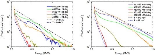
Figure 18. The electron spectra recorded in different shots at two selected viewing angles: +21° (left pane), +194° (right pane). Straight lines corresponding to exponential distributions with the relevant distribution temperatures are shown to guide the eye. #52 059 (target 0.5 mm CH2, EL = 583 J, max|Ey | = 460 kV m−1), #52 036 (target 1 mm CD2, EL = 602 J, max|Ey | = 450 kV m−1), #52 040 (target 0.2 mm CH2, EL = 583 J, max|Ey | = 250 kV m−1), #52 033 (target 0.5 mm CD2, EL = 577 J, max|Ey | = 230 kV m−1), #52 061 (target 0.05 mm Cu, EL = 597 J, max|Ey | = 220 kV m−1).
Download figure:
Standard image High-resolution imageIt may be of interest to compare our measurements to results obtained in similar conditions in other experiments. The hot electron generation at PALS was intensively investigated experimentally and through simulations within the program of studies related to SI mechanism in the inertial confinement fusion [43, 54, 55]. Under conditions similar to the present experiment except for the presence of a random phase plate and 100 µm FWHM diameter focal spot it was found for CH targets that the population of hot electrons consists of two components: the dominant one with distribution temperatures on the order of 40 keV, originating from the SRS, and a less populous but hotter one with the temperature on the order of 90 keV, generated via the TPD. As for the escaping electrons, a recent measurement at PALS was reported in [56], in which the 1ω main beam was employed without the random phase plate and focused to a 70 µm diameter FWHM spot, with 400 ps pulse duration and 800 J pulse energy, and 0.5 mm CD2 targets were irradiated. The escaping electrons were monitored with two permanent-magnet spectrometers with the effective energy range extending to 5 MeV, positioned at the viewing angles of −26° and +194° in our convention. The observed electron spectra indeed extended up to 5 MeV and appeared in a form of two-temperature distributions, with 600 keV temperature for the lower energy component and 800 keV distribution temperature for the high-energy tail. Such high electron temperatures were attributed to the phenomenon of relativistic self-focusing; it was pointed out that the threshold for self-focusing for the PALS beam might be exceeded already 100 ps prior to the maximum of the laser pulse, at a distance of 250 µm in front of the target. This mechanism was further discussed in [57]. Another recent measurement of escaping electrons was presented in [53]: 500 J/350 ps pulses with a random phase plate and 100 µm FWHM spot diameter were used to irradiate 5 mm thick Cu targets; the electron distributions on the front side of the target peaked in the direction of the target normal, achieving temperatures in the range of 50 ± 10 keV. Finally we should also mention an older result [58], where 1.053 µm wavelength beam focused to a focal spot 70 µm in diameter, with 600 ps FWHM duration and 100 J pulse energy, was used to irradiate 1.5 µm Mylar foils, and permanent-magnet spectrometers were used to characterize the ejected electrons. Electron energies up to 1.25 MeV were recorded with the distribution temperatures 90–100 keV. The high-energy component was strongly peaked along the target normal on the front side and back side of the target, similarly to what was observed in our experiment.
This overview shows that despite the fact that the hot electron temperatures recorded in our experiment are rather high for a sub-relativistic laser intensity, they are not unreasonable and there are several physical mechanisms that may be invoked to explain their values. As we see, the recorded electron spectra show large variation: on some shots the maximum electron energies barely reach 0.5 MeV, while on others in the same session they apparently exceed 1.5 MeV, and we do not see a single hot electron temperature in all shots, but rather a range of temperatures extending from 60 keV to 340 keV. A possible explanation of this behavior is that the laser–target arrangement used in this experiment was operating close to a threshold for some strong instabilities, so that a small fluctuation in the pulse energy or a small change in the beam focalization could trigger a highly dynamic process resulting in very energetic electrons being ejected from the target.
For shots for which data from all spectrometers were available one could attempt to estimate the total ejected electron charge. This was done by extrapolating the dependence of the electron distribution functions on the angle relative to the laser beam and assuming axial symmetry relative to the laser beam direction. The results indicate a total charge on the order of a µC. This is less than the charge values estimated on the basis of the target neutralization current measurements reported in [13], where charges reaching 8 µC were reported for a polyethylene target. However, we have to keep in mind that electrons with energies below 50 keV are not included in our estimate as they are not recorded due to spectrometer limitations.
7. Measurement of the target neutralization current
The ejection of hot electrons from the target results in an electric polarization of the target, which in turn initiates the target neutralization current. Such current was measured in this experiment with the inductive current probe, sensitive to the derivative of the current. In figure 19 we show the output of this probe obtained in the shot #52 059, which is a good illustration of a typical measurement. The plot is dominated by a large narrow spike, which is predominantly positive, and it attains a small negative value after the spike. (The time scale was adjusted to have the large spike at 5 ns point; an absolute timing of the target current signal relative to the laser pulse and the EMP signal was not available in this experiment. The signal was normalized by subtracting the average over the (−100 ns; −10 ns) period to remove the oscilloscope offset.) Apart from the main spike also some small secondary spikes are seen, delayed relative to the main spike by approximately 10 ns. A possible explanation for these spikes is the interaction of the expanding plasma with the conducting elements inside the chamber. (The effect of plasma expansion in the PALS experimental chamber was discussed in [50].) Another possibility is that they result from reflections of the EMP signal at interconnection points somewhere between the probe and the oscilloscope, although we consider this unlikely. In the inset in figure 19 we show the Fourier transform of the dI/dt signal shown in the main graph; we comment on this plot in section 8.
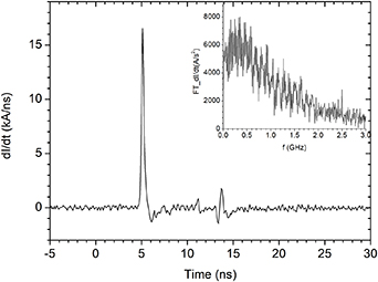
Figure 19. The derivative of the target return current I as a function of time, as measured in the shot #52 059. Inset: the Fourier transform of the dI/dt signal.
Download figure:
Standard image High-resolution image
Figure 20. Illustration of the sensitivity of Aeq to the uncertainties in the parameters a1, a2, b2, and sensitivity to the variation of f0 between 2.5 and 5.5 GHz in the interpolation formula described by equation (B.2).
Download figure:
Standard image High-resolution image
Integration of the dI/dt data shows that the target current rapidly increases to multi-kA level, reaching ∼5.7 kA level in the case of #52 059, with the 10%–90% rise time ∼400 ps. This is slightly longer rise time than reported in [40] where it was found that on the rising edge the target current signal follows the laser intensity curve. After the peak the target current decreases slowly over the period of 10s of ns, which is related to the fact that the current derivative attains there a small negative value. However, the performance of the probe in this experiment not fully satisfactory, because the current obtained from the integration of the probe signal does not fall to zero even for longer times, but we were unable to pinpoint the cause of this behavior.
8. Discussion
In section 4 we found that EMP pulses recorded inside the experimental chamber have a wide spectrum with a dominant contribution between 0.5 GHz and 2.4 GHz and some narrow spikes in this range, as illustrated in figure 11. In figure 12 we see the time-frequency analysis of the same signal, where it is evident that strong contributions near 1.0 GHz, 1.6 GHz and 2.1 GHz are present from the start of the signal. It is an obvious question how these spectra did arise. A widely accepted view [11] is that a dominant role in the generation of EMP is played by the target neutralization current. Indeed, one may invoke some heuristic arguments linking the characteristic laser and target parameters to features in the EMP spectra. For example, the target holder used in the shot #52 059 was 63 mm long; assuming that upon charging through laser–target interaction it conducted an oscillating discharge current and acted for a brief time as a quarter-wave antenna, we may relate it to the frequency of 1.2 GHz. Another characteristic parameter is the time scale of the laser pulse: the time interval of 2 × tFWHM ≈600 ps corresponds to the frequency of 1.7 GHz. However, a definitive answer should come from the comparison of the EMP spectrum with the spectrum of the neutralization current (or its derivative). Unfortunately, the result is disappointing. As may be seen in the inset in figure 19 the spectrum of dI/dt obtained for the shot #52 059 and representative for the current data in other shots in our experiment is rather featureless and does not resemble in any way the EMP spectrum shown in figure 11. We may look back to a similar measurement of the neutralization current at PALS, performed with a different target current probe, reported in [40]. The spectrum of dI/dt presented there (figure 4(a)) shows more diversity than the plot in the inset in figure 19, being dominated by a broad shoulder below 0.6 GHz, followed by a lower peak centered at 0.8 GHz and further smaller peaks extending between 1.3 GHz and 1.6 GHz. However, this plot is not easy to reconcile with figure 11 as well. We have to conclude that the available data on the neutralization current measurement at PALS do not provide a compelling evidence in support of the widely accepted picture that the dominant source of EMP is the target neutralization current.
It may well be that the experimental setup used for the neutralization current measurement was not optimal for the measurement of its high-frequency component and that future measurements with an improved setup would give a better picture of the neutralization current spectrum. Improvements could include a refined current probe design, increased bandwidth in the path between the probe and the oscilloscope, using an oscilloscope with higher bandwidth and higher sampling rate, and increasing the accuracy of the measurement in the time interval after the main spike by recording the low-level signal on a separate channel. It seems, however, that ideas for additional mechanisms of EMP generation at laser parameters relevant to this experiment should be given a serious consideration. For example, multi-GHz electromagnetic oscillations of a capacitively coupled target irradiated by a 3.5 ns pulse of an Nd-YAG laser at 5 × 10¹⁵ W cm−2 laser intensity were reported in [59]. Authors attributed this emission to oscillations of a double layer (sheath) that forms on the target surface at the laser spot upon laser irradiation. Another interesting possibility is that multi-GHz emission is related to the highly filamentary structure of the currents flowing within the expanding ablative plasma, which has been recently highlighted in [53]. One should also consider the possibility that the dynamic processes taking place in the ablated plasma plume that is still being irradiated by the laser, discussed in [56, 57], result not only in the ejection of highly energetic electrons, but may also induce a strong electromagnetic emission. We could also build upon an observation made in [25], where the effect of strong quasi-static magnetic field generation via the neutralization current induced by irradiation of a 50 µm thick macroscopic Cu plate with the PALS laser beam was considered. It was found in [25] via numerical simulation that low-energy electrons ejected from the target are confined for some time to the target surface by the target charge, forming a sheath that extends well beyond the laser focal spot. Oscillations of such a sheath are also a potential source of an electromagnetic emission, with a part of the target holder acting as a plasma antenna. Finally, the idea much studied in [6] that a significant part of the EMP might be generated by fast electrons hitting the chamber walls and exciting the chamber eigenmodes should be reassessed.
It should be pointed out that in the case that any of the mechanisms mentioned above would be proven to be physically valid, our approach to the EMP estimates in the laser parameter region where fast electron generation due to plasma instabilities is relevant would need to be modified. The assumption that the dominant source of EMP is the target neutralization current leads to the conclusion that at the given laser pulse energy strong EMP may be expected only at short-pulse facilities, as has been discussed in [11]. This follows from the fact that the cooling time of MeV electrons in typical targets is on the order of 10 ps, while the target neutralization time in the case of a 5–10 cm long target support may be estimated to be on the order of 150–300 ps (provided that the target support inductance is small). Hence in facilities with laser pulse duration on the order of 10s of fs to 10s of ps the charge accumulation phase is temporally separated from the target discharge. This results in a very large but strongly damped neutralization current pulsation that generates very strong EMP. On the other hand, for pulse duration significantly longer than the target neutralization time the charge is not accumulated on the target and the magnitude of the neutralization current is determined by the balance between the electron ejection rate and the neutralization process. The neutralization current is then quasi-stationary and does not generate strong EMP. The EMP summary data shown in figure 75 in [11] seems to be consistent with this picture; we see that in facilities with laser pulse duration on the order of 10s of fs to 10s of ps the magnitude of EMP scales—very approximately—linearly with the pulse energy, entering MV/m region for kJ pulses, whereas at the ns facilities the EMP levels are much lower and for example at the National Ignition Facility the EMP amplitudes do not increase when the pulse energy is changed from 200 kJ to 1 MJ (although for a clearer picture one should take into account in this plot in a systematic way the size of the target chamber and location of the EMP diagnostics relative to the target). This picture gives clear indication as to what should be the strategy with respect to the EMP mitigation. If it turns out there are other processes that contribute to strong EMP, this strategy may need to be changed. The results obtained in our experiment indicate that the EMP effects could be strong also for laser pulse durations that are on the order of the target neutralization time and at sub-relativistic laser intensities, provided that fast electron generation due to plasma instabilities is possible. Indeed, the EMP values we report here, i.e. ∼600 kV m−1 generated with ∼600 J pulse, when inserted in figure 75 of [11] would fall into the strip of values characteristic for the high-power short-pulse facilities. This observation could be of importance for planning experimental campaigns on laser facilities that would come online in near future, such as the S3-L4n laser at ELI-Beamlines facility in Prague [60], which would operate in a region of laser parameters that would partially overlap with the PALS parameters.
9. Summary and conclusions
Summarizing, we reported on EMP measurements at the PALS facility performed with two conductive Prodyn FD5C D-dot pencil probes, arranged in an antiparallel way. Measurements were performed inside the experimental chamber (figure 8) and outside the chamber (figure 3) in a large chamber window, with an electronic setup that guaranteed 6 GHz bandwidth. A very good signal-to-noise ratio (17:1) was obtained after some steps were taken to ensure proper EMP shielding of the data collection setup (figure 17). The signals from probes in antiparallel arrangement turned out to be remarkably consistent (figures 6 and 10), which provides a strong argument for the overall consistency of our measurement and a convincing demonstration of the usefulness of conductive electromagnetic probes for EMP measurements in kJ-class laser facility. Electric field strength values were estimated in the time domain. The EMP signal in the time domain was found to have the form of a sharp initial spike, followed by gradually decaying oscillations interspersed with some secondary spikes, which are presumably reflections of the primary spike reverberating in the chamber (figures 5 and 6). The maximal values of the vertical component of the electric field strength were obtained for a variety of plastic and metal foil targets and a massive Cu target. The highest value recorded in our experiment was  kV m−1 at a distance of 40 cm from the target, in a shot on 0.125 mm CH2 target with EL = 595 J, and the highest value recorded outside the chamber in the chamber window was
  kV m−1 in a shot on 0.06 mm Au target with EL = 615 J. It was observed that plastic targets—particularly the 100s of µm thick plastic foils—tend to generate stronger EMP fields than Cu or Au targets (figures 13 and 14). In the frequency domain it was found that the spectrum of the signal is essentially contained between 0.5 GHz and 2.4 GHz, with pronounced features near 1.0 GHz (figures 7 and 11). A clear distinction could be made between spectral features present from the beginning of the signal—such as narrow features near 1.0 GHz and 1.6 GHz—and features that appear only after some time (∼10 ns) after the start of the signal (figure 12). We found that the exact origin of the features present from the start of the signal is debatable, and further experimentation is needed to clarify the relevance of the neutralization current for this emission. The features delayed in time are likely to originate from resonance field excitation inside the chamber and interaction of the expanding plasma with fine elements present in the chamber. A full quantitative explanation of the observed effects is not yet available. This would require, first of all, a larger set of data on full field vectors in several points inside the chamber. Secondly, a fully satisfactory measurement of the neutralization current should be obtained, which is not an easy task, given the fact that the available probes are sensitive to the derivative of the current and the measurement has to capture both the huge initial spike, which requires a large attenuation, and the low-level evolution extended over a period of 10's of ns, which requires high resolution for small values of the signal. Thirdly, a good microscale model of fast electron generation and retention and plasma evolution just after the shot is necessary, which is a non-trivial issue on which a considerable progress is being presently made with the use of femtosecond polaro-interferometry [53, 61, 62]. Finally, a 3D simulation of electromagnetic fields and currents inside the target chamber should be done, with the electron and ion propagation properly accounted for, which is a very challenging task. We hope that our investigations would be helpful in preparing experimental campaigns at laser facilities that would come online in near future, such as the P3-L4n laser at the ELI-Beamlines facility in Prague [60], as well as future studies on SI at large scale laser fusion facilities.
Acknowledgments
The measurements reported here were performed after a sequence of preparatory ride-along sessions accompanying experiments carried out at the PALS facility by Professor T Pisarczyk and his group. We acknowledge participation of M De Marco in these early preparations. P R and J B acknowledge support from the Polish National Science Centre under the grant Harmonia 2014/14/M/ST7/00024. This work has been carried out within the framework of the EUROfusion Consortium and has received funding from the Euratom research and training programme 2014–2018 and 2019–2020 under Grant Agreement No. 633053, Project IFE19.CCFE-01. The views and opinions expressed herein do not necessarily reflect those of the European Commission. This scientific work was partly supported by the Polish Ministry of Science and Higher Education within the framework of the scientific financial resources in the year 2020 allocated for the realization of the international co-financed Project No. 5118/H2020/EURATOM/2020/2. The research leading to these results has received funding from the Czech Republic's Ministry of Education, Youth and Sports (Projects LM2018114 and CZ.02.1.01/0.0/0.0/16_013/0001552) and from the Czech Science Foundation (Grant No. 19-02545S). This research was also supported by the Access to the PALS RI under the EU LASERLAB IV project (Grant Agreement No. 654148) and by the Ministry of Science and Higher Education, Republic of Poland (Decision No. 3880/H2020/2018/2).
Data availability statement
The data that support the findings of this study are available upon reasonable request from the authors.
: Appendix A
The discrete Fourier transform, in which a sequence of N data points gk, k =0, 1...N − 1, is converted into a sequence of N DFT points Gn, n = 0, 1...N − 1, is usually defined as follows:
where j denotes the imaginary unit and C is a positive normalization constant. Let us assume that gk
values correspond to a discretization over N points of some continuous function g(t) that is non-zero only for ![$t \in \left[ {0,T} \right]$](https://content.cld.iop.org/journals/0741-3335/63/8/085015/revision4/ppcfac087fieqn29.gif) , i.e.
, i.e.  , where
  . One may ask how are the DFT values Gn
related to the continuous Fourier transform of g(t), defined as follows:
. One may ask how are the DFT values Gn
related to the continuous Fourier transform of g(t), defined as follows:
Let us define a sequence of N points in the frequency space,  . Approximating the integral in equation (A.2) by a left-endpoint Riemann sum over n we find:
If we choose the normalization  , our DFT values would be to a good approximation equal to the discretization of the continuous Fourier transform. The advantage of such normalization is that the DFT spectra of the same physical continuous signal obtained with the use of oscilloscopes having different sampling rates are directly comparable, which facilitates comparison of results obtained by different groups in different experiments.
: Appendix B
The equivalent area of the FD5C D-dot probe was found to be frequency-dependent. The expression obtained from a comparison with the reference Prodyn AD70 D-dot probe for frequencies below 2 GHz has the form [44]:

where f is in MHz, 
 , and
, and  . The value obtained from equation (B.1) for f = 2 GHz is higher than the datasheet value. Assuming that the datasheet value is attained at some frequency above 2 GHz we use an interpolation function of the following form:

with a suitably chosen parameters a, f0 and fs. Typically we use f0 = 3.0 GHz and fs = 0.5 GHz. In order to estimate the uncertainty in the EMP values resulting from this interpolation we vary the f0 parameter in the range 2.5–5.5 GHz.