
Abstract
A runaway electron (RE) fluid model is used to perform non-linear magnetohydrodynamic simulations of a relativistic electron beam termination event in JET. The case considered is that of a post-disruption low density cold plasma in the runaway plateau phase, wherein high-Z impurities have been largely flushed out via deuterium second injection (Shot:95135). Details of the experiment are found in separate publications. Our studies reveal that a combination of low plasma density and a hollow current profile which is confirmed by experimental studies causes fast growth of a double-tearing mode, which in turn leads to stochastization of the magnetic field and a prompt loss of REs. The phenomenology of events leading to the crash and the timescales of the dynamics are in excellent agreement with the experiment. Simulations also indicate significant toroidal variation in RE deposition but without localized hotspots. The strong stochastization setting in first from the edge leads to a poloidally broad deposition footprint that partly explains the benign nature of the termination event. This work further supports the potential possibility to engineer a benign RE beam termination scenario via deuterium second injection in ITER, as proposed by Reux et al 'Runaway electron beam suppression using impurity flushing and large magnetohydrodynamic instabilities' (submitted to Physical Review Letters).
Export citation and abstract BibTeX RIS

Content from this work may be used under the terms of the Creative Commons Attribution 4.0 licence. Any further distribution of this work must maintain attribution to the author(s) and the title of the work, journal citation and DOI.
1. Introduction
Disruptions in tokamaks occur as a result of magnetic field stochastization caused by large scale magnetohydrodynamic (MHD) instabilities [1, 2]. This leads to a loss of most of the plasma thermal energy on a millisecond timescale, cooling it to a temperature  [3]. While initial thermal losses are dominated by transport along stochastic field lines, the post thermal quench temperature evolution is determined by the relative magnitudes of Ohmic heating and impurity radiation [4]. The temperature drop increases the electrical resistivity of the plasma by several orders of magnitude, causing the plasma current to decay on a resistive timescale, referred to as the current quench (CQ). Increased resistivity also causes a large toroidal electric field, which can accelerate suprathermal electrons to relativistic velocities and energies of a few tens of MeV. The post thermal quench temperature via the impurity density and species play a crucial role here. Such runaway electrons (REs) could eventually form a beam carrying a large fraction of the pre-disruption current in fusion grade devices such as ITER [5–7]. Uncontrolled loss of REs can cause localized wall damage [8–10] and significant machine downtime. Hence the necessity to devise robust RE avoidance/mitigation strategies, motivating an improved understanding of plasma dynamics during the lifetime of the RE beam. The interplay between REs and plasma instabilities becomes important in this respect.
Several strategies have been proposed over the years for RE avoidance or mitigation [5, 11–13]. A potentially promising one has been demonstrated in a series of recent experiments at JET [12]. It has been observed that second injection of deuterium into an established post-disruption RE beam (created via high-Z impurity injection earlier in the discharge) can lead to benign terminations, i.e. without any wall damage. This can be attributed to a significant flush-out of high-Z impurities in the stationary beam phase followed by a large MHD instability causing RE losses. The lost REs are supposedly not replenished via reacceleration, mainly due to the deficiency of high-Z impurities [12]. In order to be able to potentially replicate similar benign terminations in ITER, it would be important to understand the MHD activity causing the RE losses. This is the focus of the present work.
In this paper, we present 3D non-linear MHD simulations of one such experimental shot at JET leading to a benign RE beam termination. Simulations are performed using the JOREK code [14–16]. JOREK is an extended 3D MHD code based on fully-implicit time stepping, and a spatial discretization with two-dimensional (2D) isoparametric Bezier Galerkin finite-elements in the poloidal plane and a Fourier decomposition in the toroidal direction. REs are treated via a fluid model self-consistently coupled to MHD within JOREK [17] (a kinetic model [18, 19] too is available in JOREK, but without back coupling to the plasma so far). The aim here is to shed light on the conditions causing the large instability and the ensuing non-linear dynamics until the final RE loss.
The paper is organized as follows. Section 2 summarizes the essential details of the experiment being simulated (refer to [12, 20] for further details), followed by a description of the MHD model and equilibrium in section 3. Simulation results and analysis is provided in section 4, followed by concluding remarks in section 5.
2. Experiment
The experimental shot of interest in this work is #95135 at JET, in which a disruption is triggered by the injection of massive amounts of argon impurities in the form of shattered pellets. This causes a thermal quench and a prompt conversion to a runaway current beam over the CQ (see figure 1). During the plateau phase of the RE beam with a plasma current  , deuterium shattered pellets are injected into the beam (second injection). After the second shattered pellet injection (SPI), it has been observed that most of the argon impurity species are flushed-out from the plasma due to recombination [12, 21]. The flush out of argon impurities causes a significant drop in the hard x-ray (HXR) signal as shown in figure 1(c), as Bremsstrahlung from REs is a strong function of the high-Z impurity content. The drop in HXR causes an associated drop in the rate of photoneutrons released by the interaction of HXR with Beryllium wall material as shown in figure 1(b). Expulsion of significant amount of high-Z impurities also reduces the effective resistivity and leads to a gradual increase in the plasma current [12, 21]. After about
  from the second SPI trigger, when the plasma current reaches
  , a fast and near-complete loss of REs from the plasma is observed. This is followed by a benign termination of the discharge in a few tens of milliseconds, without any localized damage on the first wall surface. The sudden loss of REs causes a large spike in the neutron count and HXR signals, as can be seen in figure 1. After the fast loss of REs, further on, there is no indication of the presence of any REs as seen from the infrared synchrotron images. This indicates that as impurity radiation is reduced significantly after the flush-out, the resulting lower toroidal electric field renders avalanche regrowth of REs from remnants ineffective.

Figure 1. Time traces of (a) plasma current, (b) neutron rate, (c) HXR signal, and (d) line-averaged electron density from the experimental shot #95135. The time corresponding to  in the discharge is taken as reference. The dashed vertical line represents the instant of
  SPI.
SPI.
Download figure:
Standard image High-resolution image3. MHD model and starting equilibrium
We use an ansatz based reduced MHD model in JOREK for the simulations, with a single fluid representation of the background plasma consisting of thermal ions and electrons. For simplicity, since the thermal pressure is too low to affect the dynamics, the background plasma density ρ and temperature T are assumed to be time invariant. The magnetic field  and electric field
  are, respectively, represented as


where, R is the major radial coordinate, ψ is the poloidal magnetic flux, F0
u the electric potential,  a unit vector in the toroidal direction and F0 a constant. The ion fluid velocity
  consists of the leading order
  drift and is given by
where B is the magnitude of the magnetic field. REs are represented as a fluid species with number density nr
, that interacts with the background plasma through a current coupling. The total current density  can be seen as decomposed into a thermal current density
  and an RE current density
  as
as

where e and c are electron charge and speed of light, respectively, and  is the unit vector along the magnetic field. Transport of REs is described here by a large parallel diffusion
  as an ad-hoc to the computationally more demanding parallel advection, which is also an option in the JOREK RE fluid model. As described in [17], use of parallel diffusion that ensures transport timescale equivalent to advection at speed of light, can adequately capture the stochastic loss of REs along the field lines with some limitations (these aspects are discussed later in this paper). Furthermore, REs are assumed to have a constant parallel momentum, and RE sources are neglected.
For our simulations, we choose a starting point that represents the plasma state a few milliseconds before the final crash. As indicated earlier, most of the argon impurities are experimentally observed to be lost by this time. Therefore we do not model impurities in the present simulations. Additionally, presence of neutrals in the plasma are not considered. The equations governing the coevolution of MHD and REs are given in normalized form by


We retain the same names for the normalized variables for simplicity. Details of normalization are provided in appendix  and
and  , respectively, while iD
is a boolean value to switch between parallel advection and parallel diffusion for RE density. A small perpendicular diffusion is used for RE density for numerical stability, via the diffusivity
, respectively, while iD
is a boolean value to switch between parallel advection and parallel diffusion for RE density. A small perpendicular diffusion is used for RE density for numerical stability, via the diffusivity  . For ηh
and
. For ηh
and  , small enough values are used such that the dynamics remain unaffected.
As mentioned earlier, we start with an equilibrium corresponding to several milliseconds before the crash, with  and q0 = 5.3. It is a challenge to obtain direct information regarding the central safety factor q0 and the shape of the q-profile from the experiment. This however, can be partly resolved through indirect evidence related to MHD mode structure and synchrotron emission before the crash. This is described in the following.
Excellent data on synchrotron radiation acquired during the SPI RE experiments at JET, especially using the IR camera (KLDT-E5WC, λ = 3–3.5  ) allows to discriminate some of the RE beam properties. Despite the fact that synchrotron radiation pattern and intensity is a function of multiple variables—local magnetic field direction and intensity, RE energy, pitch angle and local RE density on one side and the camera properties on the other—it is possible to infer various qualitative observations from the image data and forward synchrotron pattern modeling using, e.g. SOFT code [22]. Simulations were performed using SOFT Green's function tool to reconstruct the synchrotron images that would result from different RE density profiles (including JOREK equilibrium profile) and different regions of phase space allowed. Figure 2 shows the original camera image with subtracted background and the reconstructed image from JOREK equilibrium. Clearly, a qualitatively good match is observed with the JOREK profile. The results here corresponds to a moderate pitch angle range θ = 0.1–0.3 radians and lower energies (1–15 MeV). However, it is observed that the conclusions hold true also in the case when contributions from higher energy or higher/lower pitch angle populations are considered. SOFT simulations were repeated (for the set of RE density profiles described in appendix
- (a)Low pitch angle (0.1–0.3 rad), low energy 0.5–15 MeV
- (b)Low pitch angle (0.1–0.3 rad), high energy only 20–25 MeV
- (c)High pitch angle (0.3–0.6 rad), low energy 0.5–15 MeV
- (d)High pitch angle (0.3–0.6 rad), high energy only 20–25 MeV.

Figure 2. (a) Infrared synchrotron image from the experiment (Shot:95 135), corresponding to the JOREK equilibrium time point  in figure 1; (b) reconstructed synchrotron image from SOFT simulation, with JOREK equilibrium RE density profile as input.
Download figure:
Standard image High-resolution imageIn all of these cases, hollow profiles provide synchrotron images that were very distinct from those obtained from any peaked profile in the IR camera spectral sensitivity band—crescent-like shape (as the one observed in experiment) extended to the top and bottom parts of the circular cross-section could be achieved only by a hollow profile. Images from the peaked profile were far from experimental observation throughout the studied phase space. Furthermore, comparison with other RE density profiles considered excludes the probability of non-hollow profiles (see appendix
Furthermore, m = 4 magnetic islands visible in the synchrotron images before the crash (not shown here) provide an additional constraint on the location of the q = 4 surface, that can only be satisfied by a hollow profile. In fact, the equilibria with hollow profiles feature two q = 4 surfaces and the location of the inner one is able to explain the experimental structures. JOREK MHD test simulations (not shown here for brevity) with a monotonous current profile for the equilibrium obtained from EFIT did not reproduce the correct dynamics as in the experiment. For example, these simulations showed a dominant (m, n) = (2, 1) mode as compared to the dominant (m, n) = (4, 1) mode observed in the experiment, and also did not result in any stochastization of the plasma. On the other hand, simulations with different hollow profiles recover these dynamics in a very robust way as shown later i.e. the results are not strongly sensitive to the value of q0. To summarize, the SOFT simulations, observation of m = 4 islands and JOREK test simulations provide sufficient evidence for the existence of a hollow current density profile before the crash. Hence only hollow profiles are considered henceforth.
Further constraints are necessary in order to completely define the current/q-profile. This is provided by information on the MHD modes as observed from the infrared synchrotron data over a time span of a few tens of milliseconds starting before the crash. This is shown in figure 3 which shows the approximate minor-radial location of the m = 6, m = 5 and m = 4 islands during various time points until the crash, where m is the poloidal mode number. The islands shown here correspond to the n = 1 toroidal mode, so that m = q, the safety factor. It has been observed that the m = 6 islands move radially outward and eventually leave the plasma in  , as shown in figure 3. Following this, the m = 5 islands are visible which again move radially outward. They are invisible after around
  , but are still within the last closed flux surface. Finally, before the crash (indicated by the red vertical dotted line), m = 4 islands are visible at much lower minor-radial locations. This provides an approximate location for the inner q = 4 surface for the equilibrium being sought.

Figure 3. (a) Approximate minor radial location of the m = 6, m = 5 and m = 4 structures at various time points until the final crash, as deduced from magnetic island structures observed in the infrared synchrotron images. The time corresponding to  in the discharge is taken as reference. (b) Synchrotron images showing the m = 6, m = 5 and m = 4 island structures, highlighted by the 'star' symbols.
Download figure:
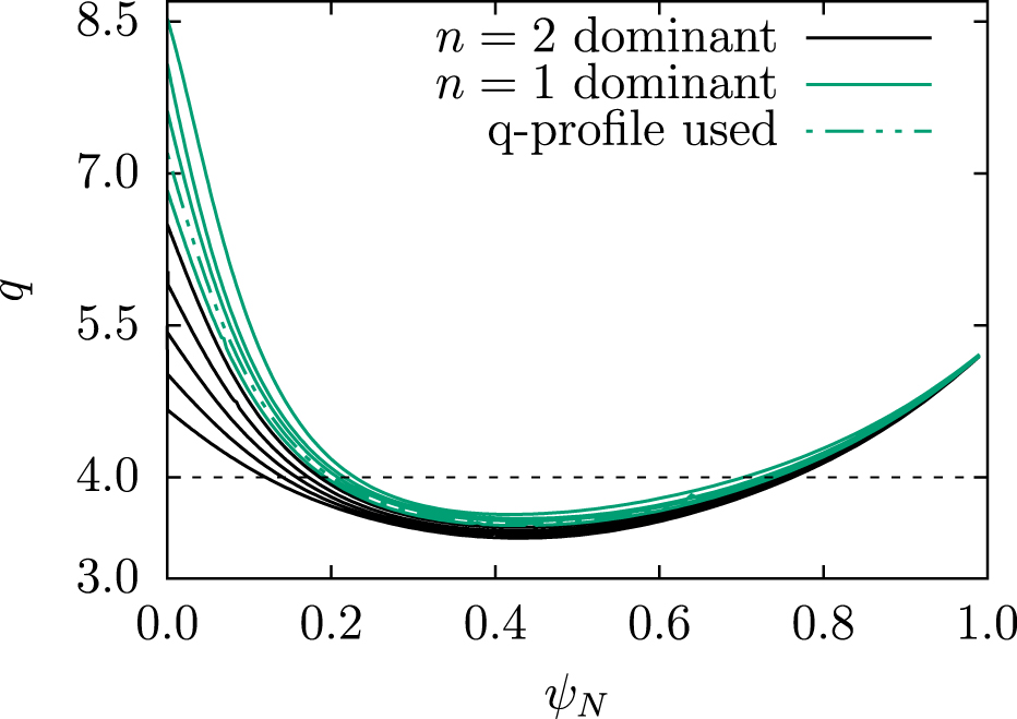
Standard image High-resolution imageA scan of q profiles with the q = 4 surface in the vicinity of  have been performed to determine the non-linearly dominant toroidal mode in the JOREK simulations (shown in figure 4). It can be seen that with an increase in q0, beyond a threshold, there is a clear transition in the most unstable MHD mode, from an n = 2 dominant behavior to an n = 1 dominant behavior. In line with the aforementioned experimental observation of n = 1 dominant mode before the crash, one of the q-profiles (green colored lines) would satisfy now all the known constraints. Furthermore, it is seen from the sensitivity test that the final results of interest are not very sensitive to the precise profile chosen among the plausible ones. This enables us to choose the dotted profile (in figure 4) as representative of the equilibrium before the crash.

Figure 4. Safety factor profiles used to study the sensitivity of MHD linear instability on the central safety factor q0. For q0 above a certain threshold, there is a transition from n = 2 dominant (black curves) to n = 1 dominant (green curves) behavior.
Download figure:
Standard image High-resolution image4. Simulation results
The computational domain used is shown in figure 5(a) colored by the normalized RE density at equilibrium, along with the flux surfaces. The boundary of the domain closely approximates the first wall surface. The runaway beam is nearly circular and approximately  in diameter. The plasma current
  and the on-axis toroidal magnetic field
  . Being a cold plasma, the equilibrium is practically pressure-less. The corresponding equilibrium safety factor and current density profiles are summarized in figure 5(b). The background plasma density
  . The resistivity and viscosity are spatially uniform, with values
  (which corresponds to a Spitzer value at
  ) and
) and  . All the current is assumed to be carried by REs at the initial state. Runaway parallel diffusion is chosen to be
  which is
  , where
  is an appropriate length scale for stochastic parallel transport or connection length. Simulations were performed including toroidal modes n = 0, ..., 8 on a poloidal grid
  with radially local clustering to resolve resonant surface regions. A dedicated grid sensitivity study showed no noticeable change in linear growth rates with further increase in grid resolution.
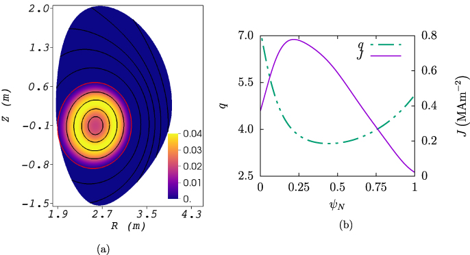
Figure 5. Starting equilibrium state for the simulations: (a) Computational domain of JOREK colored by normalized RE number density nr , shown along with the flux-surfaces. The red curve represents the last closed flux-surface; (b) profiles of the safety factor q and the current density J as a function of the normalized poloidal flux ψN .
Download figure:
Standard image High-resolution image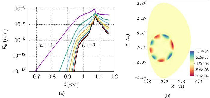
Figure 6. (a) Toroidal modes n = 1 to n = 8 of the energy in the poloidal magnetic field Eb
as a function of time; (b) mode structure at the end of the linear phase ( ) of the
  at the outer q = 4 surface shown colored by the non-axisymmetric part of the RE number density nr
.
at the outer q = 4 surface shown colored by the non-axisymmetric part of the RE number density nr
.
Download figure:
Standard image High-resolution imageFigure 6(a) shows the evolution of the energy in the poloidal magnetic field (in the toroidal modes n = 1, ..., 8) with time. It can be seen that the most unstable mode is the (m, n) = (4, 1) double tearing mode, dominant primarily at the outer q = 4 surface as shown in figure 6(b). Being a relatively low density plasma, the Alfvén timescale is much smaller ( ) and hence the tearing mode growth rate is relatively faster than in a typical density scenario. Via a test in the linear phase, we confirmed that the n = 1 growth rate using parallel diffusion is similar to that with advection at the speed of light (less than 2% difference). Running the full simulation with advection is possible, but computationally too expensive with the existing numerical methods. Additionally, the growth rate is found to increase with parallel transport in line with the prediction of the linear theory by Zhao et al [23]. Growth of the n = 1 mode triggers the linear growth of the subsequent toroidal modes in order until saturation. Subsequent non-linear interaction triggers stochastization of the magnetic field. Magnetic island structure at the early non-linear phase (
 ) with the (4, 1) and (5, 1) islands is shown in the poincare plot in figure 7 (panel (a)). It is observed that stochastization starts initially around the outer q = 4 surface (panel (b)), and extends inwards toward the core (panel (c)). REs are lost as the field stochastizes. Since REs are lost much faster from the stochastic regions than from within the island regions, differential loss of REs can be observed from the localized high density of REs in the islands (panel (c)). Subsequent to this, the core (region still retaining the closed flux surfaces) shrinks until it reaches a size of a few centimeters of diameter (panels (d) and (e)). This observation matches well with the core-shrinking also seen during the final crash in the experiment. By this stage, about 94% of the REs are lost from the plasma. Stochastic loss of REs happens over a total time span of approximately
  . From the simulations, the core-shrinking is seen to occur as a series of instabilities of sequentially higher poloidal mode numbers. For example, between the span of a few tens of microseconds between panels (c) and (e) of figure 7, islands corresponding to n = 5, n = 6 and n = 7 are broken successively leading to the core-shrinkage.

Figure 7. Poincare plots at different time points from the MHD simulation showing magnetic island formation, stochastization of the magnetic field leading to fast RE losses and the subsequent reformation; (a) t = 0, (b)  , (c)
, (c)  , (d)
, (d)  , (e)
, (e)  , (f)
, (f)  . Early non-linear phase (simulation time
  ) corresponding to (a) is taken as reference time t = 0. Background color indicates the magnitude of RE density nr
.
) corresponding to (a) is taken as reference time t = 0. Background color indicates the magnitude of RE density nr
.
Download figure:
Standard image High-resolution imageThe corresponding evolution of total plasma current and RE current is shown in figure 8. The quick loss of RE current is accompanied by a reformation of thermal current during this duration via the induction effect. A small Ip spike ≈3% is observed in the simulation as a result of magnetic helicity conservation, which is similar to the Ip spike that appears after the thermal quench of a disruption. The time resolution of the current from the experiment is insufficient to conclude if such a short timescale Ip spike actually occurred in the shot. However, Ip spikes (of magnitudes between 1% and 8% of Ip ) have been observed in other discharges from the series of experiments described in [12, 20]. After the crash, the thermal plasma current decays at the resistive timescale. Accurate modeling of the downstream process requires the inclusion of Ohmic heating, radiative losses etc in the simulations and is not of interest for the present work.

Figure 8. Evolution of the total plasma current and the RE current. The experimental current is shifted in time for clear comparison.
Download figure:
Standard image High-resolution imageThe RE loss during the crash is accompanied by a current profile flattening due to fast magnetic reconnection [24]. This is shown in figure 9(a) along with the corresponding q-profiles in figure 9(b) at various instances of time during the losses. It is interesting to note the minor-radially inward shift of the peak of the current profiles with time (or the location of high shear in q profile). This correlates to the previously mentioned sequence of instabilities with increasing poloidal mode number that causes the core-shrinking. We now turn to the impact of the stochastic RE losses on the wall.

Figure 9. (a) Current density profiles, and (b) safety factor profiles shown at different time instants during the non-linear and RE loss phase, showing the profile flattening due to fast magnetic reconnection. Reference time t = 0 is the same as in figure 7.
Download figure:
Standard image High-resolution imageFigure 10(a) shows the distribution of toroidally-averaged RE flux ( ) on the wall during the time span of the RE loss, as a function of the poloidal location and time. It can be seen that most of the RE flux occurs in the near limiter region until ψN
≈ 1.2 (or a poloidal distance of
) on the wall during the time span of the RE loss, as a function of the poloidal location and time. It can be seen that most of the RE flux occurs in the near limiter region until ψN
≈ 1.2 (or a poloidal distance of  ), which can be considered as a poloidal broadening of RE flux. This partially explains the reason for the low impact of REs on the first wall in this termination event, in addition to the absence of RE re-acceleration due to lack of high-Z impurities. It must be noted that the use of parallel diffusion as an ad-hoc leads to RE losses deposited on both sides of the limiter point (up and down), as opposed to the way deposition would occur with parallel advection of REs. In our analysis, this effect is accounted for by mapping the RE flux on both sides of the limiter to a single side, as per the ψN
value of the location. Furthermore, it is observed that large RE losses occur within a duration of
), which can be considered as a poloidal broadening of RE flux. This partially explains the reason for the low impact of REs on the first wall in this termination event, in addition to the absence of RE re-acceleration due to lack of high-Z impurities. It must be noted that the use of parallel diffusion as an ad-hoc leads to RE losses deposited on both sides of the limiter point (up and down), as opposed to the way deposition would occur with parallel advection of REs. In our analysis, this effect is accounted for by mapping the RE flux on both sides of the limiter to a single side, as per the ψN
value of the location. Furthermore, it is observed that large RE losses occur within a duration of  , which matches very well with observation from the experiment. The distribution of magnetic field line connection length to the boundary, which quantifies the degree of stochasticity, also supports this observation (see appendix

Figure 10. (a) Distribution of RE flux (particles per square meter per unit time) as a function of the normalized poloidal flux ψN (or distance from the limiter point) and time during the stochastic RE loss phase. (b) Distribution of RE fluence (particles per square meter) as a function of the normalized poloidal flux ψN and toroidal angle φ during the time span shown in (a).
Download figure:
Standard image High-resolution imageFigure 10(b) shows the distribution of RE fluence (particles per square meter) on the wall during the time period shown in figure 9(a), as function of poloidal and toroidal locations. In addition to the poloidally broad deposition, there is variation of RE deposition along the toroidal direction. The poloidal broadening is due to the stochasticity setting in first at the plasma edge, unlike a situation with predominantly core-stochastization wherein the deposition would be concentrated close to the limiter point. The toroidal distribution is smooth without any localized hot-spots, and this is clearly attributed to the n = 1 mode that was dominant even through the non-linear phase.
It was verified that the overall dynamics of this beam termination event with RE parallel diffusion is very similar to that in a simulation with RE parallel advection at the speed of light (fluence could not be obtained from the advection simulation though).
5. Summary and discussion
The first self-consistent non-linear MHD simulation of an RE beam termination event in JET has been presented. Mutual interaction between MHD and REs is treated by the use of an RE fluid model. Useful insights have been obtained on the dynamics of the crash and RE loss. A low density plasma with a hollow RE current profile leads to fast MHD growth dominated by n = 1, stochastization and corresponding RE losses. This is accompanied by current profile flattening by fast magnetic reconnection. Results show a good match with experiment. RE deposition shows significant toroidal variation (but without local hotspots), and poloidal broadening that potentially reduces the RE load on the wall. This explains in part why no first-wall damage is observed in the experiment. Results presented in this work improve our understanding of specific aspects of MHD behavior and therefore contribute to the development of a safe RE beam termination scenario in high current tokamaks. This opens up new avenues toward devising a robust RE mitigation scheme for ITER.
The starting equilibrium used in our simulations is clearly representative rather than fully empirical, but sufficiently adequate for the objective of this work. Sensitivity studies confirm a weak dependence on the exact current profile. Furthermore, as previously mentioned, parallel diffusion was used as an ad-hoc to relativistic advection of REs in order to avoid excessive computational costs. Nevertheless, from test simulations with advection, it was confirmed that the dynamics remain very similar in both cases. For example, linear growth rates differed by less than 2% and the RE loss rates due to stochasticity were very similar as well. Additionally, while using parallel diffusion, sufficient care was taken to map the RE flux onto one side of the limiter, to mimic the way REs would be deposited on the first-wall in case of advection. Hence all the important physical effects (if not exact details) are still captured adequately with the use of ad-hoc parallel diffusion.
Our simulations further substantiate the broad theme proposed by Reux et al [12] on the potential utility of deuterium second injection. From this study, it is seen that an MHD instability causing strong stochastization first in the edge region (achieved by a hollow current density profile in this case) can be a very conducive ingredient to proactively enable scattered RE losses to avoid wall damage. However, it is vital to understand the physics behind the formation of a hollow profile to be able to reliably obtain it and assess the applicability of the D2 second SPI scheme in ITER. We plan to study this aspect in the future.
Furthermore, in elongated plasma scenarios such as in ITER, possible vertical instability after the first or second injection makes the applicability of the scheme challenging. Hence it is important for future studies to perform RE termination studies in elongated shapes with free-boundary computations in order to incorporate vertical dynamics realistically. Major MHD codes have demonstrated the ability to do so, including 3D instabilities in a benchmark exercise [25].
Acknowledgments
The authors acknowledge help from G Szepesi for providing equilibrium data. Fruitful discussions with F J Artola and E Nardon are also acknowledged. We also acknowledge useful suggestions on the manuscript from S Gerasimov. This work has been carried out within the framework of the EUROfusion Consortium and has received funding from the Euratom research and training programme 2014–2018 and 2019–2020 under Grant Agreement No. 633053. This work was also supported by the EUROfusion—Theory and Advanced Simulation Coordination (E-TASC). The views and opinions expressed herein do not necessarily reflect those of the European Commission.
Appendix A
Normalization used for the variables shown in the governing equations (5a )–(5f ). The factors µ0, n0, ρ0 refer to the magnetic permeability of free space, central number density and the central mass density of the background plasma, respectively, and kB is the Boltzmann constant.
| Quantity | Normalization |
|---|---|
| Time, t |

|
| RE density, nr |
|
| Speed of light, c |
|
| Electric potential, u |
|
| Toroidal vorticity, ω |
|
| Current density, j |
|
| Resistivity, η |
|
Viscosity, 
|
|
Diffusivity, 
|
|
| Density, ρ |

|
| Temperature, T |
|
Appendix B
Some of the RE number density profiles (normalized) tested with the Green's functions are displayed in figure 11(a). Corresponding to the displayed profiles a series of synthesized images is shown in figure 11(b). Although only qualitative comparison has been conducted, it is obvious that any kind of peaked profile cannot create the observed radiation pattern given the diagnostics parameters.

Figure 11. (a) Normalized RE density profiles as a function of the normalized radius ρ = r/a. The hollow profile r/a = 0.5 corresponds to the equilibrium profile used in JOREK. (b) Reconstructed (synthetic) synchrotron profiles from SOFT simulations corresponding to the profiles shown in (a).
Download figure:
Standard image High-resolution imageAppendix C
The evolution of the connection length distribution during the stochastic RE loss phase is shown in figure 12. Smaller connection length corresponds to a higher degree of stochasticity. It can be observed that stochasticity in the radially inner regions only last for  , as also indicated by the flux deposition.

Figure 12. Distribution of field line connection length lc (m) to the boundary as a function of ψn and time.
Download figure:
Standard image High-resolution image