Spatiotemporal Analysis of Climatic Extremes over the Upper Indus Basin, Pakistan

Abstract

The Hindukush-Karakoram-Himalayan (HKH) ranges and their massive cryosphere extend over the Upper Indus Basin (UIB) and are prone to incapacitated water supply due to the proclivity of globally increased temperature. Due to excessive carbon emissions, frequent incursions including extreme climatic events, are likely to happen sooner than expected on a regional scale due to recent climate change. The present study examined the variability of climatic extremes (18 indices) during 1971 to2018 over the UIB. The Mann-Kendall (MK) test and Sen’s methods were applied for statistical analysis as the former deals with the magnitude of trends while the direction of observed trends was identified by the latter in climatological time-series data. The frequency and intensity of summer days (SU25 > 25 °C/year) at 13 out of 27 stations significantly increased, particularly in lower regions. The same warming proclivity was dominant in tropical nights (TR20 > 20 °C/year) at 20 stations including Astore, Bunji, Gilgit, Gupis, Murree and Skardu. Similarly, significant increases were observed in extremes of annual precipitation in western and high northern areas; however, significantly, the highest drops in R25 and R5day were exhibited in Chitral at the rates of 13 and 29 days, respectively. These findings tend to support the accelerated summer warming and a rather stable winter warming while stable winter warming showed that overall the UIB seems to be more sensitive towards warming.

1. Introduction

The increasing temperature makes Pakistan highly vulnerable in response to changing climate. The global temperature increased by 0.89 °C from 1901 to2012 [1]. Such a high-level increment in temperature not only influences the seawater and wind circulation at the global scale but also affects regional-scale climate. Weather and climate events occur in response to natural variability and anthropogenic climate changes [2].

Previously, a significant number of studies conducted in Pakistan concerning analysis of hydro-climatological trends have been conducted in Pakistan [3,4,5,6,7,8,9,10,11,12,13], revealing an increasing trend of extreme temperatures. Previously [14] indicated the increasing trend of extreme temperature in Pakistan [14]. Pakistan is partitioned into five locales. The northern parts, southwestern parts included Baluchistan Level, and the upper and lower Indus fields have a warming pattern yet, shockingly, northwestern sloping territories showed a cooling pattern in January. In addition, the northern and western rough domains of the nation demonstrate bigger inter-annual temperature variability. Similarly, Ref. [6] exhibited that patterns of anticipated temperature and rainfall along the scope (north–south). The anticipated temperature ascends all through Pakistan in one decade from now might be ascribed to provincial atmosphere changes, an unnatural weather change [8,15].

Global warming causes heat waves and high flooding in response to extreme weather regionally. Particularly, extreme warming (temperature) and severe droughts (precipitation) events occurred in last few decades. These heat waves were high intensity while drought period was consistent and lasted longer than usual [7,16]. Extreme climate events and abrupt weather variability may have calamitous impacts on various potential sectors of water resources, agriculture, energy, economy, health and infrastructure [2,11,16]. Spatiotemporal variation in meteorological variables resulted in weather extremes in Pakistan too. In 2017, Turbat, Blaochitan province exhibited 54 °C in 2017. This temperature was not only the highest temperature ever recorded in Pakistan so far but the hottest temperature on the earth’s surface in Asian continent. Similarly, in the same year a severe heat wave was observed as 50 °C in southern areas of Pakistan as the highest temperature in April. Moreover, 620 mm of 24-h rainfall event was observed in Islamabad on 23 July 2001 [7]. Developing countries are sensitive to extreme weather and climate change due to limited resources, which enhances further economic loss. IPCC Third Assessment Report [17] revealed significantly decreased frequency of the monthly and seasonal temperatures extremes globally in 19th century. However, during latter half of 20th century a 2–4% increase in the frequency of heavy precipitation was observed over the Northern Hemisphere. Around 0.6 °C increment in January temperature was seen during 1961–2006. In Gilgit Baltistan-Azad Kashmir (GB-AK), Balochistan, KP-TA, Punjab and Sindh mean decadal temperature peculiarities were 0.10 °C, 0.23 °C, −0.15 °C, 0.06 °C and 0.16 °C, respectively. The highest temperature irregularity was observed in the southwestern part of Sindh (Karachi) attributed to urban warmth island effect. During the recent three decades, western parts of Balochistan, including Chaghi and Quetta demonstrated highest temperature inconsistencies between 0.5 °C to 1.5 °C in January. Several previous investigations widely used the Mann-Kendall (MK) test for trends evaluation of extreme temperature and precipitation [18,19,20,21,22,23,24,25,26]. Previously [20,21] indicated the changes in wet/dry periods and extreme temperatures during 50 years using the same MK test. Similarly, [27] used the pre-whitening test to eliminate the effect of autocorrelation time series data. After removing the influence effect, a trend test was applied. Many studies also used the pre-whitening test [28,29,30,31,32,33]. Recently, a study in this region addressed the temperature and precipitation extremes using a similar method of MK test for trend significance (1980–2019) [34]. They observed spring as the hottest season which exhibited warm nights at the rate of 0.49 °C/decade. It’s worth mentioning that previous studies were mainly restricted to particular climate variability in terms of a single variable and extreme weather events in UIB. These studies addressed overall trends and extreme analysis based on single climatic variables. The present study seeks spatial variability in trends of observed maximum/minimum temperature and precipitation concerning hot/cool and wet/dry days, respectively in UIB Pakistan. We used extreme temperature and precipitation indices for station data from 1971 to 2018. The used dataset features an updated record with a wide coverage of daily temperature and precipitation observatories in selected areas of UIB. Based on the updated analysis, we address the inter-annual and seasonal variability of extreme events of temperatures and precipitation

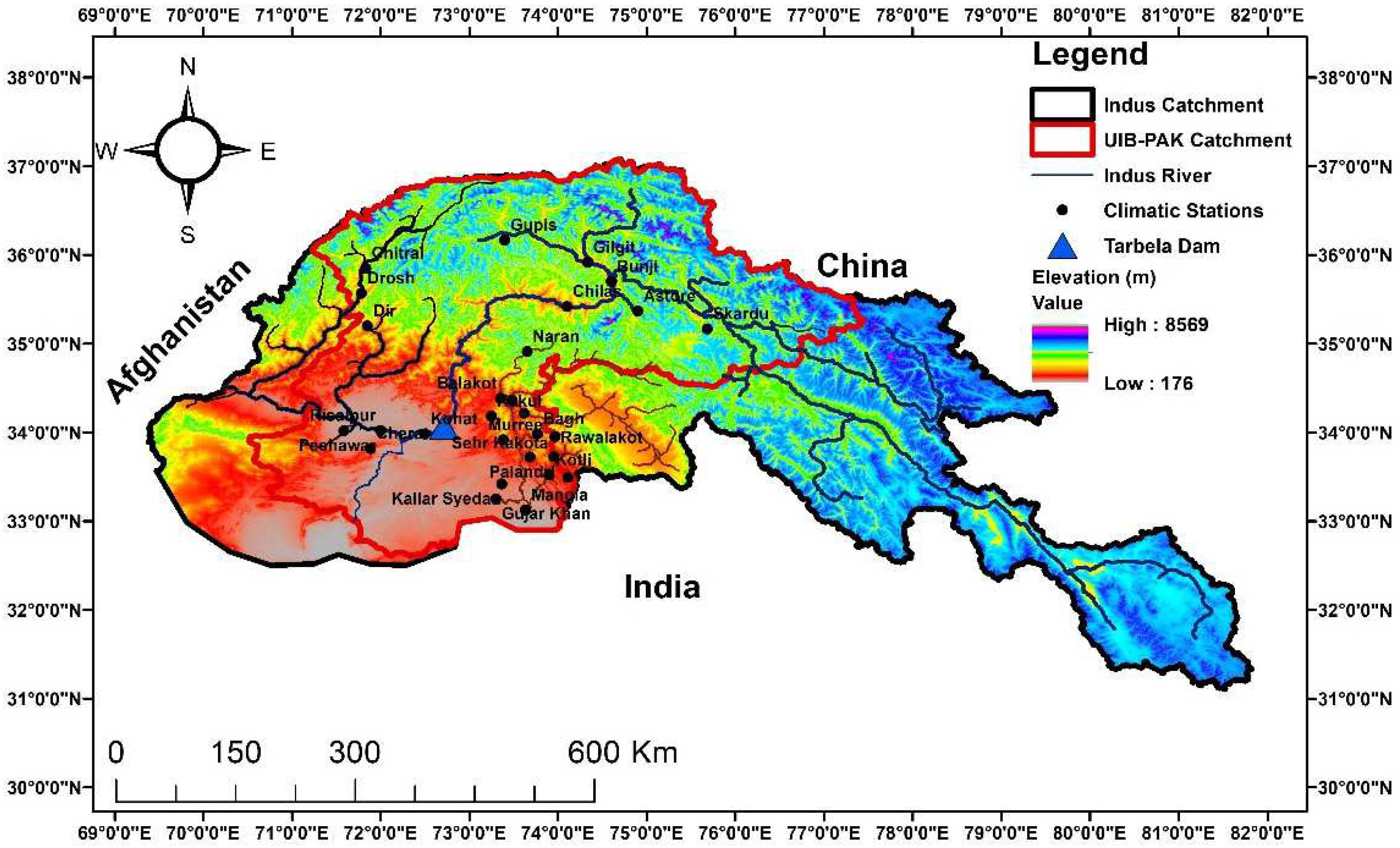
2. Study Area and Datasets

The Indus is considered to be one of the biggest transboundary basins which encompasses 1.1 × 10⁶ km² sharing borders with its neighbours; Afghanistan (6.7%), China (10.7%), India (26.6%), and Pakistan (56%) [35]. The Indus River is 3180km long, flowing from the northern Tibetan Plateau to India, and finally enters into the Pakistan’s territory at the Kharmong flow gauging station [36].

The catchment area upstream of Tarbela Dam is referred to as the Upper Indus, while downstream is called Lower Indus Basin. Geographically, it is situated between 33°40′ to 37°12′ N latitude and 70°30′ to 77°30′ E longitude in the HKH region. The upper Indus Basin also serves as the Water Tower of Pakistan due to the vast size of its glacier, which supplies water for water resources (reservoirs) and hydropower generation. The melt-water produces runoff from the UIB and precipitation in winter primarily consists of solid/liquid snow. The melt process in summer for snow and glaciers is generally initiated in the mid to late ablation period. The runoff volume is reliant on winter snow and subsequent temperature in spring to summer. The study area is shown in Figure 1.

We used daily data for the trend analysis with temperature and precipitation being the core variables. The description of each climatic station is given in

Table 1. Meteorological stations used in UIB.

Station	Latitude	Longitude	Elevation	Mean Annual Temperature			% of Missing Values
	(dd)	(dd)	(m)	Max. Temp (°C)	Min. Temp (°C)	Rainfall (mm)	Max. Temp	Min. Temp	Rainfall
Astore	35.2	74.5	2168	15.6	4.0	482	3.1	3.3	0.1
Bagh	34.0	73.8	1067	21.7	12.4	1440	2.3	2.2	2.2
Balakot	34.6	73.4	996	24.9	11.9	1563	0.4	0.1	0.7
Bunji	35.6	74.6	1372	23.8	8.4	175	0.4	0.4	0.2
Cherat	33.5	71.3	1372	21.4	14.4	608	2.1	1.7	0.1
Chilas	35.3	74.1	1250	26.4	14.1	192	2.0	0.7	7.7
Chitral	35.9	71.8	1498	23.3	8.6	471	0.6	0.7	2.8
Dir	35.2	71.9	1375	22.9	8.0	1356	0.7	0.4	0.2
Drosh	35.4	71.7	1462	24.1	16.0	593	0.7	0.5	0.4
Garidopatta	34.2	73.6	814	25.9	12.2	1487	1.2	3.7	2.2
Gilgit	35.6	74.2	1460	23.9	7.7	137	0.8	0.3	0.1
Gujar Khan	33.3	73.3	457	28.7	14.9	815	2.3	0.2	2.7
Gupis	36.1	73.2	2156	18.8	6.6	188	1.3	0.8	1.0
Kakul	34.1	73.2	1308	23.0	10.8	1302	0.8	0.8	0.1
Kohat	34.0	72.5	1440	29.6	17.1	696	0.4	1.6	0.2
Kotli	33.5	73.9	610	28.4	15.8	1230	2.0	0.5	3.8
Mangla	33.1	73.6	282	29.7	17.3	849	0.3	0.3	0.2
Murree	33.9	73.4	2206	17.2	8.7	1748	1.5	2.2	1.4
Muzaffarabad	34.4	73.5	702	27.6	13.6	1483	1.5	0.9	2.2
Naran	34.9	73.7	2363	11.8	9.1	1654	1.1	3.1	0.4
Palandri	33.7	73.7	1402	15.6	12.4	1424	0.7	0.2	0.5
Parachinar	33.5	70.1	1725	21.1	8.0	847	1.3	1.4	0.2
Peshawar	34.0	71.5	320	37.4	16.2	449	1.1	0.9	0.3
Rawalakot	34.0	74.0	1677	20.7	9.2	1349	2.3	0.1	0.6
Risalpur	34.0	72.0	575	29.7	14.5	572	1.4	0.2	0.4
Saidu Sharif	34.4	72.2	961	26.1	12.0	1066	1.9	1.1	0.3
Skardu	35.2	75.4	2317	18.6	4.9	224	0.6	0.4	0.1

dd, decimal degrees.

.

Temperature and Precipitation Extreme Indices

The frequency, intensisty, and persistence of temperature and precipitation extremes might be compromised due to the changing climate. There is no particular definition for an extreme event, however, several definitions have previously been proposed and applied [2,37]. The expert team on climate change detection, Monitoring and Indices (ETCCDMI), developed with the help of the WMO Commission for Climatology and the Research Programme on Climate Variability and Predictability (CLIVAR) 27 climate-change indices, many of which have been widely used in evaluating extreme temperature and precipitation in the Middle East, central Asia, etc. [38,39]. This method has also been applied in southeast Mediterranean climate patterns [40].

Similar definitions for extreme climate events are also seen in many other studies [41]. In the EMULATE (European and North Atlantic daily to multi-decadal climate variability) project, 64 more detailed climate indices are defined [42,43,44]. Accordingly, it was beneficial to apply various indices to obtain a broad and more reliable picture of climatic behavior in the study area.

In this study, a set of 17 indices was used to examine spatial and temporal variability of temperature and precipitation extremes. These are detailed in

Table 2. Indices for maximum and minimum temperature and precipitation extremes.

ID	Description	Unit
Maximum Temperature
SU25	Summer days (SU25), number of days with maximum temperature >25 °C	Days
TXx	Maximum value of daily maximum temperature/year	°C
TXn	Minimum value of daily maximum temperature/year	°C
TXm	Annual average maximum temperature	°C
Minimum Temperature
FD0	Frost days (FD0) Number of days with minimum temperature <0 °C	Days
TNx	Maximum value of daily minimum temperature/year	°C
TNn	Minimum value of daily minimum temperature/year	°C
TR20	Tropical nights (TR20), number of days with minimum temperature >20 °C	°C
TNm	Annual average minimum temperature	°C
	Precipitation
Rm	Annual average precipitation of all days in the year	mm
WD	Length of total rainy days/wet days with PRCP > 1 mm in the year	days
CDD	Length of total non-rainy days/dry days with PRCP <1 mm in the year	days
Rsum	Annual total precipitation.	mm
SDII	Simple daily intensity index.	mm day-1
Rx	Maximum precipitation	mm
R25	The R25, PRCP > 25 mm	days
R5day	R5day is the annual maximum consecutive 5-day precipitation amount	mm

. All these indices were calculated on an annual basis for each independent time series during the 46-year period (1971–2018). As indicated in Table 2, the indices were defined in different ways, varying from a certain fixed threshold (summer days (SU25) and tropical nights (TR20). These definitions are objective, site-independent, and facilitate direct comparisons between different regions [45]. Our study area is a typical case, whereby complex terrain and diverse climates are evident.

In contrast to other studies, our study used the extremes which exceed the generally used climatic thresholds for instance, summer days (SU25: Tmax > 25 °C), tropical nights (TR20: Tmin > 20 °C), and frost days (FD, Tmin < 0 °C). This method enables reliable assessment of climate impacts in terms of climatic variables. The following four indices (TXx, TXn, TNx, and TNn) refer to absolute values and highly sensitive data quality. We used annual precipitation as the basic indicator due to the association of annual precipitation with extreme precipitation events.

Rm is the annual average precipitation of all days in the year. WD is the length of total rainy days or wet days where precipitation is >1 mm during during a year whereas the consecutive dry days (CDD) refers to the length of total non-rainy days. A wet day refers to a day where precipitation is >1 mm within a day, while a dry day shows where precipitation < 1 mm within day. Rsum represents the total sum of all daily precipitation within a year. SDII represents the simple daily intensity index which is the average wet day precipitation intensity.

SDII is measured in millimeters mm/day. It is also called the precipitation intensity. Rx represents the highest daily precipitation within a year. The R25 exhibit threshold index refers the frequency of intense precipitation. i.e., the annual total number of days when precipitation is >25.4 mm (1 inch). R25 is measured in days. R5d represents the annual maximum consecutive precipitation amount (mm) over five days. Rm is annual average precipitation of all days in the year with units in millimeters. The consecutive dry days (CDD) is measured I, days and shows the maximum number of consecutive dry days.

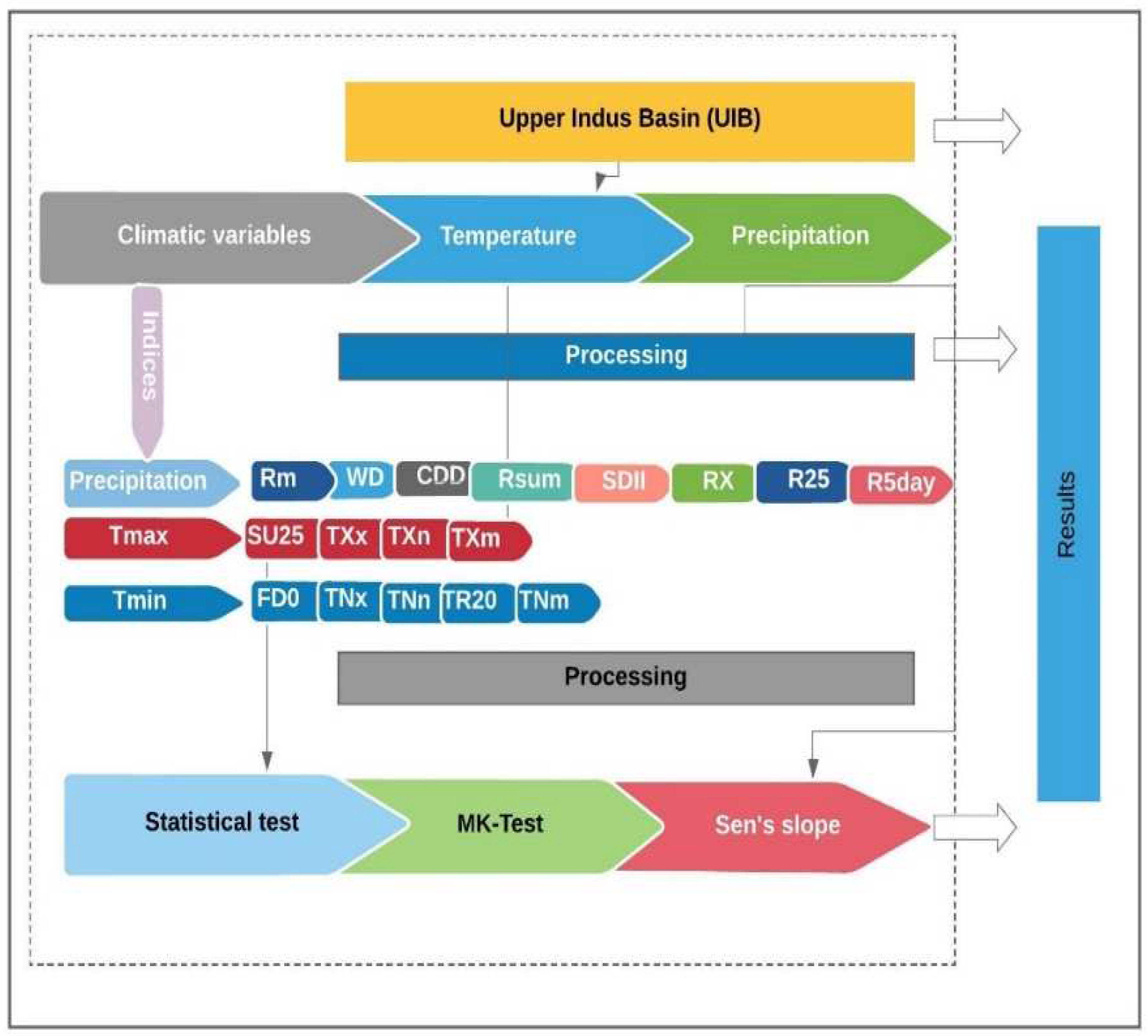
3. Material and Methods

3.1. Trend Detection

Trend identification by parametric or non-parametric statistical tests seeks the existence of significance and governs the values of a random variable which increases/decreases over a period of time in statistical terms [46,47]. The Mann-Kendall (MK) test and Sen’s robust slope estimator (SS) have been widely used in trend detection and estimation [48,49,50]. Previously [27] concluded that the results of the MK and Spearman rank correlation tests are similar. We applied these two tests for trend identification, the methodology flowchart is given in Figure 2.

3.1.1. Assessment of Autocorrelation

Autocorrelation is the mutual correlation of a variable with itself during the following time interval prior to test application. In particular, presence of the positive autocorrelation verifies the significant trend in time series data [50]. Some studies suggested the ‘pre-whitening’ of data for removing to autocorrelation [51,52,53,54,55].

The method of ‘pre-whitening’ is appliead as follows

$$Y_i=X_i-\left(\beta \times i\right)$$

(1)

The trend (β) represents slope which was calculated by Sen’s estimator to make a linear trend, given as follows

$$\beta =\mathrm{midian}\left(\frac{X_i-X_j}{i-j}\right), {\forall }_j<i$$

(2)

where 1 < j < i < n. The r1 represents the lag-1 autocorrelation. The method of data refining is applied where r1 is significant, however, in the case of insignificant r1 at the 5% level, original values will be required for test application. The pre-whitening method is applied as follows

$$\begin{gathered} {Y^{\prime }}_i=Y_i-r1\times Y_{i-1} \\ {Y^{″}}_i={Y^{\prime }}_i+\left(\beta \times i\right) \\ {Y^{″}}_i \mathrm{is} \mathrm{pre}-\mathrm{whitened} \mathrm{time} \mathrm{series}. \end{gathered}$$

(3)

3.1.2. Mann-Kendal Test for Trend Detection

The trend identification for climate change impact assessment is carried out by MK statistical test [56,57,58]. It is very suitable due to its simple data requirements such as that the data must not be normally distributed and data breaks do not compromise the results of time-series data [56].

Test statistic Zmk, is calculated using the following relation:

$$Z_{\mathrm{mk}}=\left\{\begin{array}{cc}\frac{S-1}{{\sigma }_s}& if S>0\\ 0& if S=0\\ \frac{S+1}{{\sigma }_s}& if S<0\end{array}\right\}$$

(4)

S can be found as:

$$S={\displaystyle \sum }_{k=1}^{n-1}{\displaystyle \sum }_{j=k+1}^{n}sgn\left(X_j-X_k\right)$$

(5)

where n is the number of years, x_j and x_k, are the annual values in the years j and k, respectively. The function sgn(x_j − x_k) is an indicator function that takes the value 1, 0, or −1 according to sign of difference (x_j − x_k), where j > k:

$$sgn\left(X_j-X_k\right)=\left\{\begin{array}{cc}1& if x_j-x_k>0\\ 0& if{x}_j-x_k=0\\ -1& if{x}_j-x_k<0\end{array}\right\}$$

(6)

Zmk might be positive or negative with respect to data, designating an upward (warming) or negative (cooling) trend. Significance level α of an existing trend depends upon the test statistic (S) which may follow the standard normal distribution if there is the probability under the null hypothesis Ho, of observing a value higher than the test statistic Zmk. The null hypothesis Ho stands true in the absence of a trend, Ho will be rejected. For the direction of a trend (positive/negative) a two-tailed test at α level of significance Ho is rejected if the absolute value of Zmk > Z1-a/2 at the α-level of significance.

3.1.3. Sen’s Slope Estimator

The changes over the period (1971–2018) were computed from the slope estimated by Sen’s method [48]. The slope estimates of N pairs of data using the following equation

$$Q_i=\frac{x_{j-}{x}_k}{j-k} \mathrm{If} j > k$$

(7)

where x_j and x_k represent annual values of the year’s j and k, respectively, while Sen’s shows the median of these N values of Q. N values of Qi are arranged in increasing order for slope estimation using the following

$$\mathrm{Sen}’\mathrm{s} \mathrm{estimator}=Q_{\left[\left(N+1\right)/2\right]} \mathrm{if} N \mathrm{was} \mathrm{odd} \mathrm{and}$$

(8)

$$\frac{1}{2}\left(Q_{N/2}+Q_{\left[\left(N+2)/2\right)\right]}\right) \mathrm{if} N \mathrm{was} \mathrm{even}$$

(9)

Lastly, two-sided test at 100 (1 − α) % is applied to assess Qmed at the certain confidence interval.

3.1.4. Inhomogeneity and Change-Point Analysis

The homogeneity of climatic records might be affected by the method of gauging and data collection, the conditions around the station, the station location, and the reliability of the measurement tools. Homogeneous climate time-series may be defined as the series only influenced by the variations in climate. For this reason, the reliability and quality of the data taken from the observation stations need to be tested statistically prior to their used in hydrological modelling and research studies. It can be stated that the natural structure of the observation values does not deteriorate when the climatic time-series have a homogenous structure. Homogeneity is important in detecting the variability of the data. The homogeneity tests are classified into two groups: absolute tests and relative tests. In the absolute method, different tests are applied separately for each station while in the relative method, the neighboring (reference) stations are also used in the testing [59]. In literature, many methods such as the standard normal homogeneity test (SNHT), the Buishand range (BR) test, the Pettitt test, and the Von Neumann tests were proposed for testing the homogeneity of meteorological variables such as precipitation and temperature [60,61,62,63,64]. These methods have been often applied in studies aiming to analyze the variability in the hydro-meteorological time series over different regions of the world [65,66,67,68,69]. We have used XLSTAT for trend analysis, slope detection, and change-point identification.

4. Results

We analyzed changes in climatic extremes for the selected weather stations in different sub-basins of the UIB, as shown in Figure 3. The maps show the magnitude of positive/negative changes in detected trends at selected locations.

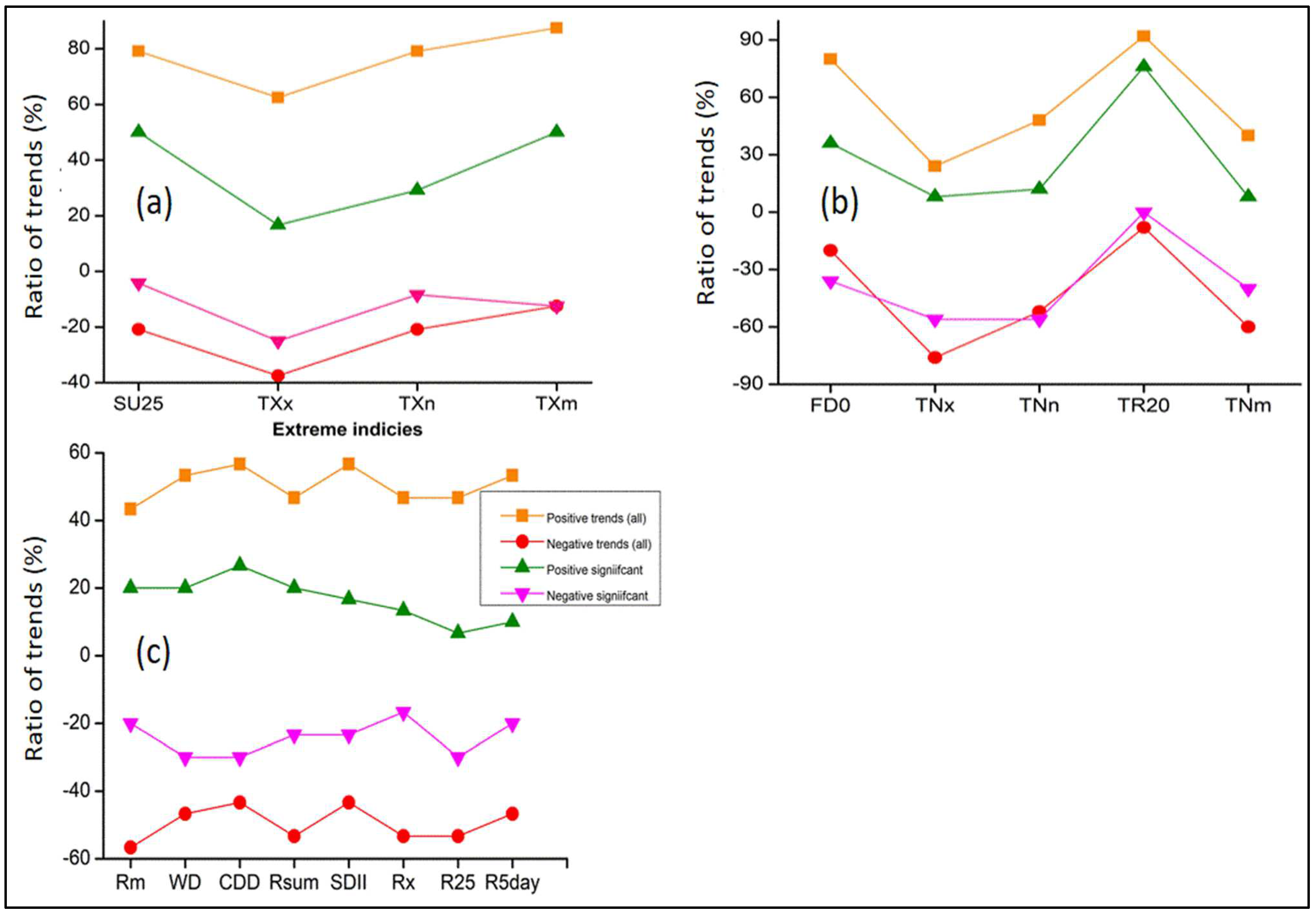
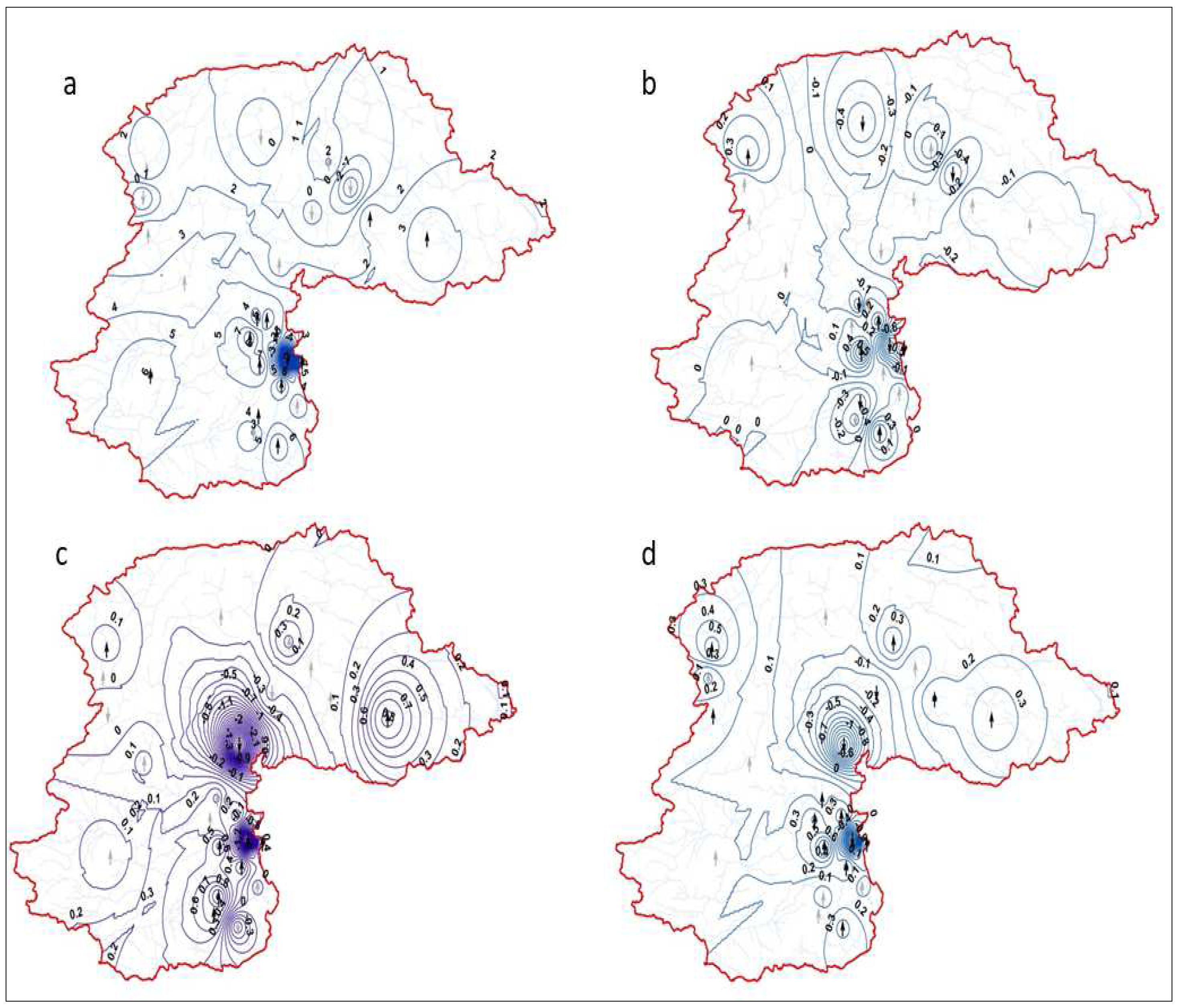
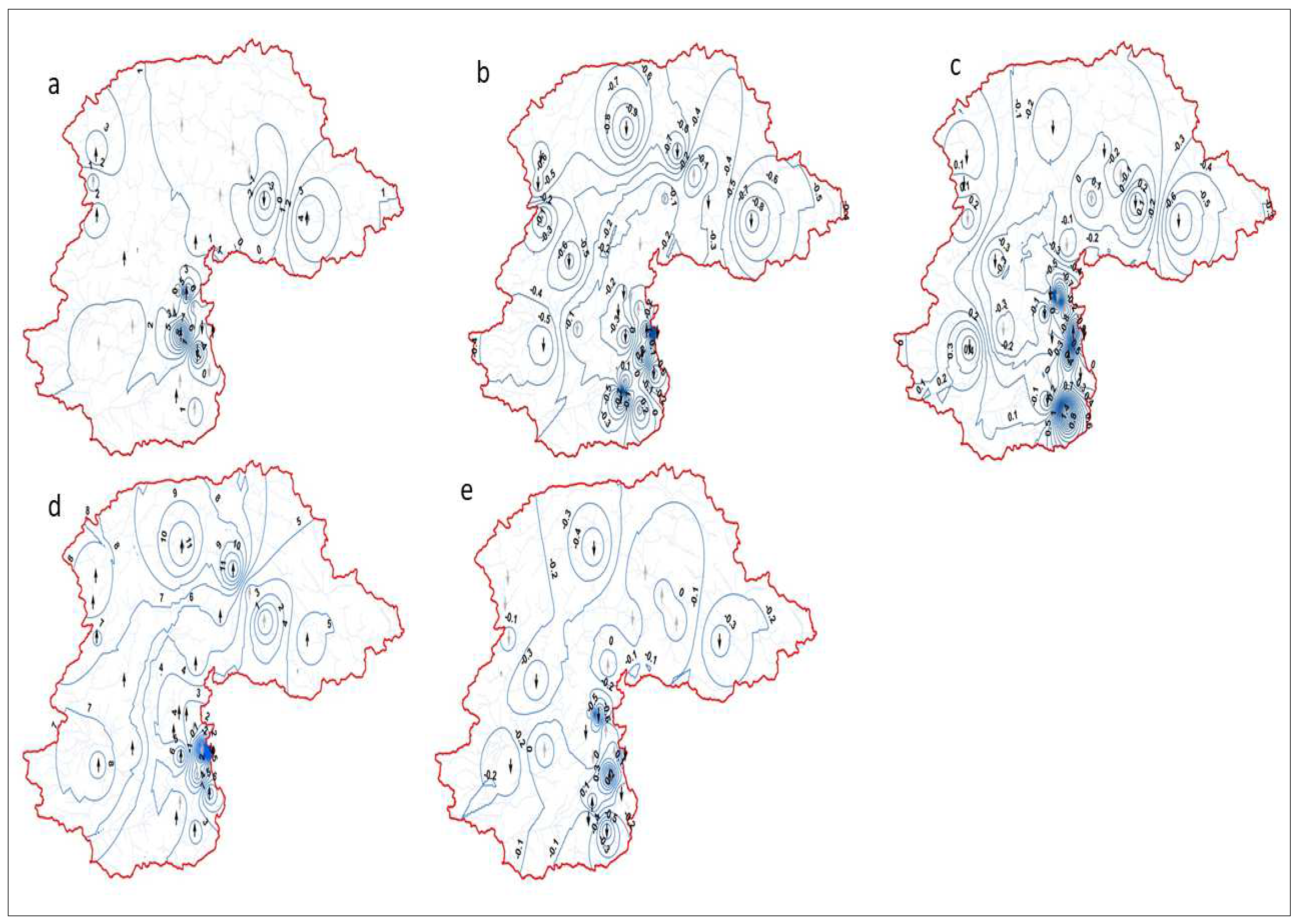
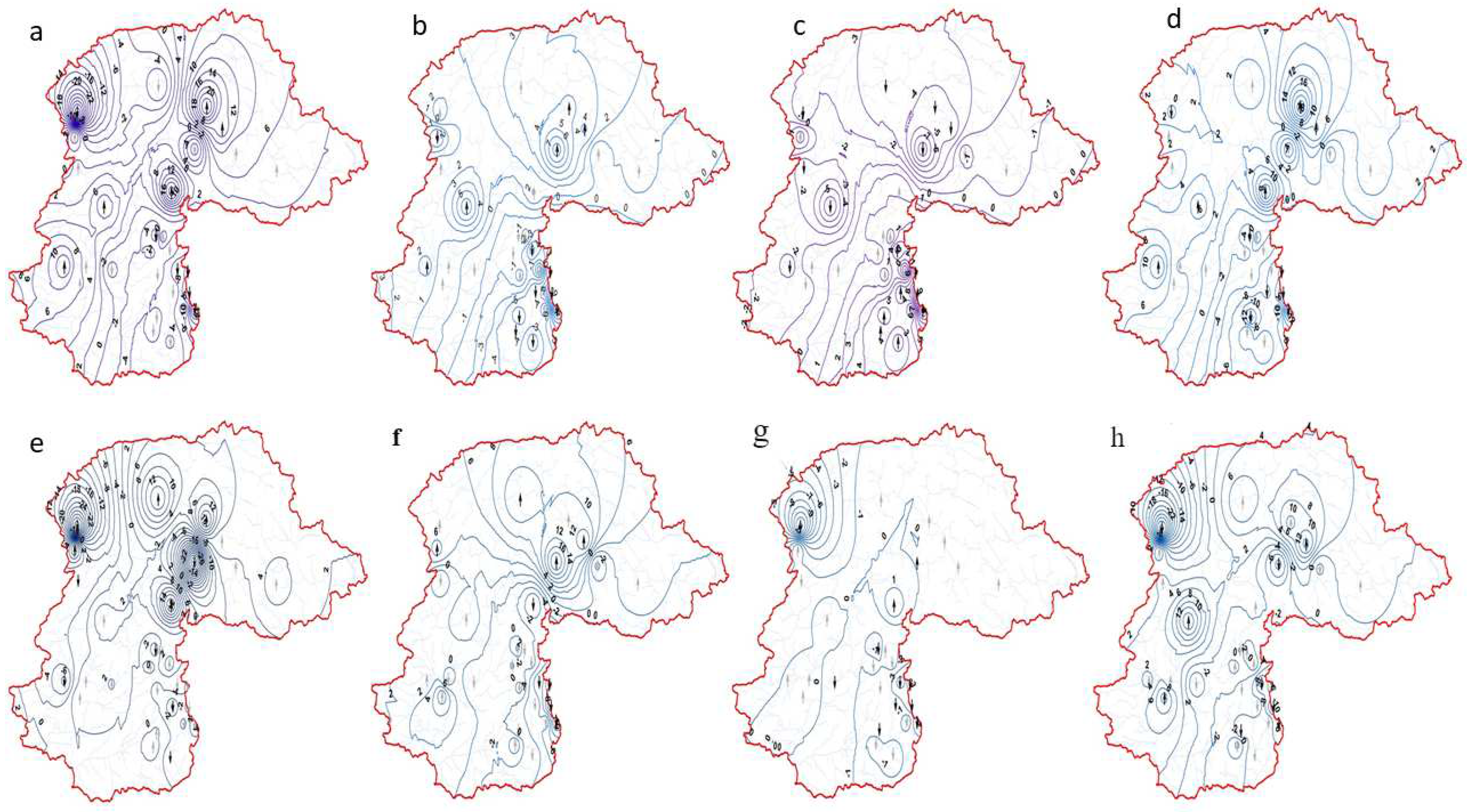
4.1. Extreme T_max Variablity

We observed significant upward trends in most of the temperature extremes. On average, such increases were prominent for summer days (SU25), TXx, TXn, and TXm during 1971 to 2018. Figure 3a also indicates that SU25 and TXm increased significantly at more than 50% of the stations. Similarly, TXx and TXn were significantly increased at 20% and 30% of the stations, respectively. On the other hand, these extremes were negative at fewer than 20% of the stations. These trends support the concept of warming prevailing at most of the stations in terms of increasing numbers of summer days and annual average maximum temperature in UIB.

We observed a prominent warming pattern in all indices of Tmax during 1971 to 2018; in particular, the warming signal was stronger at Mangla Kotli and Kallar as shown in Figure 3. Similarly, some stations including Astore, Murree and Naran exhibited a strong cooling signal. TXm for Naran has been decreased but increased for Murree during 1971–2016. Similarly, the number of SU25 for Murree and Naran increased.

The variation in climatic extremes at a different location is attributed to land-use changes, vegetative cover, and urbanization in the UIB. Most of the stations exhibited positive trends with a large variation in magnitude at the regional scale. More warming trends were found in the lower region of the UIB compared to the higher region. We found that summer day SU25 extremes showed positive trends at most of the stations as shown in Figure 4a. The highest number of decreasing SU25 was seen at Bagh with a rate of 15.4 days per decade (significant with p < 0.01). However, Rawalakot showed the highest increasing trend (significant with p < 0.01) at the rate of 14.4 days per decade.

TXx, TXn, and TXm are changing throughout the UIB revealing a substantial inconsistency spatially in hot extremes. The trend value in TXm varied from −1.3 to 0.7 °C per decade. A statistically significant increase in TXm was experienced at twelve stations and trend values varied up to 0.7 °C per decade, while only three stations Naran, Bagh and Chilas showing a negative trend.

4.2. Extreme T_min Variablity

We observed that most of the cold extreme indices exhibited a decreasing trend. Significantly increasing trends were found for frost days (FDo) and tropical nights (TR20) at 80% (36% were significant) and 92% (76% were significant) of the stations, respectively, for the 1971–2018 period whereas TNx, TNn, and TXm showed more negative trends at 20% (56%), 48% (56%) and 42% (40%) of the stations, respectively. In contrast, FDo, TNx, TNn, TR20 and TNm increased significantly at the rates of 72, 64, 68, and 48% of the observatories, respectively, including both warming and cooling trends. We noted a similar prominent warming pattern in all indices of Tmin to those observed for Tmax. In particular, the warming signal was stronger in TR20 at most of the stations, however, FD0 exhibited overall cooling patterns, as shown in Figure 5. The cooling tendency was prominent in TNm, TNn, TNx at Astore, Saidu Sharif, and Naran but warming was observed in FD0. The highest temperature drop was observed at Skardu for both time-series, followed by Bagh and Murree.

The spatial patterns in minimum temperature trends for the frost days (FDo) exhibited negative trends on eastern side of the UIB along the line-of-control (LOC). The rest of the stations revealed positive trends, as shown in Figure 5a. Significant decreased FDo were experienced at Astore (significant with p < 0.05), Bagh (p < 0.1), and Plandri (p < 0.05) with the rate of 3.5, 0.2, and 4.5 days per decade, respectively. In contrast, increased FDo were observed at Chitral (p < 0.05), Dir (p < 0.1), Gujar Khan (p < 0.05), Murree (p < 0.001), Muzaffarabad (p < 0.01), Naran (p < 0.1), Rawalakot (p < 0.001), Skardu (p < 0.01), and Saidu Sharif (p < 0.001) with rates of 3.9, 2.3, 0.4, 10.1, 6.4, 0.4, 0.2, 4.0 and 1.2 day per decade, respectively. Figure 4 also depicts the extreme of annual high minimum temperature across the whole region. Just two stations Bagh (p < 0.1) and Plandri (p < 0.05) exhibited a warming pattern at 0.5 and 0.4 °C per decade, respectively. The spatial variation of trend value varied from −1.3 to 0.5 °C per decade.

The downward trend in TNx was associated with decreasing temperature at night, which increased frost days and extension of cooling duration, with snowfall duration. Trends of low minimum temperature were similar to those of high minimum temperature extremes. The highest rate of decrease was observed at Muzaffarabad (p < 0.001) with the rate of 1.4°C per decade. However, for the trend of tropical nights TR20, warming was experienced across the whole of the UIB. No significant cooling trend was observed.

4.3. Variability in Extreme Precipitation

We observed a consistent pattern of mixed trends, particularly for, Rm, Rsum, Rx, and R25 for which downward trends prevailed, while the other four extreme indices WD, CDD, SDII and Rx exhibited upward trends at most of the stations. The Rm showed more negative trends at 57% of the stations but only 20% were observed as significant, as shown in Figure 3c.

We found an overall decreasing pattern, spatially and temporally, as shown in Figure 6. Rx and R5day increased at Astore, Bagh, and Balakot, however, Rsum and Rm increased markedly in Naran. We observed that WD and R25 increased markedly at Naran and Chitral stations, respectively, as shown in Figure 6b,g.

We found significant WD at nine station across the entire UIB. The number of WD increased significantly at a few stations, but decreased at many stations. The CDD showed significant positive trends at 27% of stations and the same pattern was found in intensity index SDII at 30% of stations. The Rx and R25 decreased at 53% of the stations.

Total precipitation might be associated with changes in the frequency of rainy days or average intensity of the events. For further verification of this, trends in annual number of rain days and average daily precipitation during rainy days was calculated during the study period. Except in eastern UIB, rainy days significantly increased supporting increased precipitation frequency in most of the regions.

The wet/rainy days (WD) exhibited a decreasing pattern in eastern UIB mainly in the catchment area of the Mangla Dam while the rest of the UIB exhibited increased rainy days. We observed that average daily rain rate and rainy days were similar and increased significantly over almost all the UIB except for some stations in the Jhelum basin.

We also found the annual frequency of extreme precipitation days, R25 (Figure 6g), was the same as that of annual total precipitation (Figure 6d). The varied from −3.5 to 2 days per decade.

Decreasing trends appeared over the lower eastern part of the UIB, mainly in the Mangla catchment, however, increasing trends were observed, mainly located in the western and upper regions. The trend variation in highest precipitation, from −14% to 18%, also increased in the higher western and northern regions of the UIB while lower and eastern region had decreasing trends, as shown in Figure 6f.

5. Discussion

We observed the recent changes in climatic extremes in terms of precipitation and temperature all over the UIB during 1981–2018. According to updated analysis, we noted a significant increase in summer days and warming trends in annual average temperature at 13 stations. These findings are consistent with [70], who reported seven stations exhibiting warming trends in annual maximum temperature within the UIB. A similar dominance of warming trends at lower altitude stations was revealed by a study during 1981–2013 [30]. Our finding of significant warming of tropical nights (TR20) also supports the idea of winter warming during 1967–2005 suggested by [14]. The significant increases in warming trends of the present study are also endorsed by the extent of the shrinkage of global spring-snow cover in Northern Hemisphere [2] and the UIB/Gilgit Basin [33,71]. The increase in night temperature has led to a limited new snow events ultimately resulting in less snow cover. Warmer days expedite the snow melting process so the snow cover is decreasing all over the UIB. Similar consistent increase in maximum temperatures and warming patterns were observed at high altitude regions of Khunjrab and Naltar [30]. An increasing number of TR20 over the UIB might be attributed to cloud cover, short/long-wave radiation, and energy budget. Some authors [71] observed decreases in daytime cloud cover and increases in low-level cloud at night. The warming of tropical nights is associated with such phenomena. Our findings of increasing summer-days are fully consistent with the results of [30] who reported significant autumn warming and significant positive trends at Astore, Bunji, and Saidu Sharif during the previous two decades (1991–2013).

The progressive warming supports rapid the melting of the Himalayan, Hindukush, and Karakoram glaciers, resulting in glacial lake outburst flood (GLOF), jeopardizing the neighboring towns and roads (e.g., the Shishper glacier). The effect of temperature variation on snow accumulation is difficult to estimate accurately due to large variations in precipitation amount and phase (solid/liquid) according to changing altitude [72,73,74]. Increasing temperatures may create serious concerns regarding early spring snowmelt and glacier melting in the ablation period, which results in flooding. Some recent studies suggested that increased runoff in Gilgit Basin with snow/glacier melt contribution attributed to increased temperature [33]. The precise snow and glaciers melting assessment requires remotely-sensed data in combination with field-based estimates of melting rates of snow, permafrost, and glaciers which might be employed in future studies.

We must control anthropogenic activities in downstream areas to maintain a sustainable environment under this changing climate. Being an agricultural country, our farming community will be compromised in upstream and downstream areas, particularly in arid regions where most crops are precipitation-dependent. Increasing summer days will reduce soil moisture memory (persistence to hold moisture) of cultivated lands which will ultimately lead to barren lands. Increased summer days will reduce the duration of winter season so there will be less solid snow accumulation in the winter. Furthermore, the reduced accumulated snow will melt early causing severe floods. The increasing summer temperature will further enhance the early melting rates of fresh snow and permafrost ultimately leading to rapid glacier melting. Some glacier-mass-balance studies proposed that eastern and central Karakoram glaciers exhibit glacier retreat in accordance with global glacier shrinkage trends [75]. Furthermore, recent field-based estimations [76,77,78] suggested enhanced areal coverage of debris-covered areas. One may expect due to this fact that increased summer days will enhance melting rates and a further increase debris-covered area.

Climate change in terms of increasing temperature, is occurring strikingly in the UIB. According to our key findings, most areas exhibited significant increases in summer days with negative trends in annual precipitation. Some recent and previous studies observed cooling/warming of temperature and increased/decreased amount of precipitation in the UIB, as discussed. We observed a strong relationship between precipitation extremes and total precipitation in all areas. Moreover, the total precipitation was positively correlated with precipitation extremes concerning Rx, R25, and R5 days. These trends suggest that precipitation is getting frequent but less intense at most parts of the UIB. Conversely, it is getting intense but less frequent in the Mangla watershed. The positive trends in total precipitation within the UIB generally align with increasing average precipitation frequency and intensity. We observed that negative trends in total precipitation in eastern UIB, mainly in the catchment area of the Mangla Dam are associated with a reduced number of rainy days. However, average intensity was higher but was unable to compensate for the loss of total precipitation in terms of fewer rainy days. Our results showed significantly decreasing Rx, R25, and R5 days at most of the stations. These negative precipitation extremes are consistent with regional trends suggesting spring-dying in the UIB [5,31], ultimately leading to lower crop yields in mountain agricultural areas. Our findings are consistent with recent studies [34,79,80] in terms of warm tropical nights, summer warming, and decreased precipitation. Similarly, some authors reported decreased winter precipitation but unaltered trends of annual precipitation in the Himalayan region [6]. However, we observed significantly decreased annual precipitation. As far as temperature trends are concerned, we observed a significant increase in warming days at low-altitude stations which is inconsistent with high altitude cooling trends [30] but the drop in annual precipitation is consistent with [31]. Some studies observed increased winter and monsoon precipitation [70], however, our observed trends revealed significant annual precipitation even in monsoon-dominant areas. We observed that the number of wet days has been significantly decreased in terms of R25 and R5 days which is inconsistent with [81,82,83]. Our findings of wet/dry days will further help with sustainable agricultural planning [84].

6. Conclusions

The present study focused on the variation in extreme temperature and precipitation indices over the past 48 years in the UIB, Pakistan.

According to the observations, our results agree with the regional findings observed in the Northern Hemisphere in response to global warming. We observed large variations all across the UIB attributed to changing temperature, elevation, landforms, and vegetation. The present study suggests a prevailing impact of positive trends in the frequency and intensity of hot extremes with considerable regional differences throughout the basin. Furthermore, warming trends were dominant at lower regions of the UIB compared to the higher areas. On the other hand, cold extremes exhibited a down ward trend tendency. We found the extremes largely shifted during hot season as compared to the cold season. More warming was seen through FDo and TR20 whereas, TNx, TNn, and TX exhibited more negative trends. The comparison between warming and cooling temperature extremes was directly affected by the climate change impacts. In particular, shifting in the warming tendency was more sensitive when compared to the cooling tendency.

We found significant changes in precipitation extremes concerning the frequency and intensity of hot events. Generally, positive trends in wet days and rainfall intensity dominated, while precipitation frequency decreased in the UIB. Western and higher northern areas of the UIB experienced significant increases in annual total precipitation while eastern areas, mainly the Mangla catchment exhibited significant decreases.

Increase in temperature and precipitation extremes is the major aspect of global warming. This indicates that temperatures will continue to rise in the UIB. Therefore, there is the need to build capacity and to decrease the vulnerability to extreme temperature. The major result of this investigation is the detection of the trends and variability in extreme temperature and precipitation. Therefore, this investigation was important in investigating the changes in climate hazards. It is evident that the outcomes of this study will assist in future adaptation and mitigation planning to combat the effects of extreme temperature in the UIB, Pakistan.

References

1. IPCC. Climate Change. In The Physical Science Basis. Contribution of Working Group I to the Fifth Assessment Report of the Intergovernmental Panel on Climate Change; Cambridge University Press: Cambridge, UK; New York, NY, USA, 2013; p. 1535. [Google Scholar]
2. IPCC. AR4 (Intergovernmental Panel on Climate Change Fourth Assessment Report). Climate change and water 2007. IPCC Technical paper VI. 2008. Available online: http://www.ipcc.ch/pdf (accessed on 1 January 2022).
3. Abbas, F. Analysis of a historical (1981–2010) temperature record of the Punjab province of Pakistan. Earth Interact. 2013, 17, 1–23. [Google Scholar] [CrossRef]
4. Abbas, F.; Rehman, I.; Adrees, M.; Ibrahim, M.; Saleem, F.; Ali, S.; Rizwan, M.; Salik, M.R. Prevailing trends of climatic extremes across Indus-Delta of Sindh-Pakistan. Theor. Appl. Climatol. 2018, 131, 1101–1117. [Google Scholar] [CrossRef]
5. Hussain, S.S.; Mudasser, M. Prospects for wheat production under changing climate in mountain areas of Pakistan-An econometric analysis. In Agricultural Systems; Elsevier: Oxford, UK, 2004. [Google Scholar]
6. Iqbal, M.A.; Penas, A.; Cano-Ortiz, A.; Kersebaum, K.; Herrero, L.; Del Río, S. Analysis of recent changes in maximum and minimum temperatures in Pakistan. Atmos. Res. 2016, 168, 234–249. [Google Scholar] [CrossRef]
7. Khan, N.; Shahid, S.; bin Ismail, T.; Wang, X.J. Spatial distribution of unidirectional trends in temperature and temperature extremes in Pakistan. Theor. Appl. Climatol. 2019, 136, 899–913. [Google Scholar] [CrossRef]
8. Khattak, M.S.; Ali, S. Assessment of temperature and rainfall trends in Punjab province of Pakistan for the period 1961–2014. J. Himal. Earth Sci. 2015, 48, 42–61. [Google Scholar]
9. Maida, Z.; Ghulam, R. Frequency of extreme temperature and precipitation events in Pakistan 1965–2009. Sci. Int. 2011, 23, 313–319. [Google Scholar]
10. Revadekar, J.V.; Kothawale, D.R.; Patwardhan, S.K.; Pant, G.B.; Kumar, K.R. About the observed and future changes in temperature extremes over India. Nat. Hazards 2012, 60, 1133–1155. [Google Scholar] [CrossRef]
11. del Río, S.; Iqbal, M.A.; Cano-Ortiz, A.; Herrero, L.; Hassan, A.; Penas, A. Recent mean temperature trends in Pakistan and links with teleconnection patterns. Int. J. Clim. 2012, 33, 277–290. [Google Scholar] [CrossRef]
12. Salma, S.; Shah, M.A.; Rehman, S. Rainfall Trends in Different Climate Zones of Pakistan. Pak. J. Meteorol. 2012, 9, 37–47. [Google Scholar]
13. Yaseen, M.; Tom, R.; Ghulam, N.; Rehman, H.; Latif, M. Assessment of recent temperature trends in Mangla watershed. J. Himal. Earth Sci. 2014, 47, 107–121. [Google Scholar]
14. Khattak, M.S.; Babel, M.S.; Sharif, M. Hydro-meteorological trends in the upper Indus basin in Pakistan. Clim. Res. 2011, 46, 103–119. [Google Scholar] [CrossRef]
15. World Meteorological Organization. Guide to Climatological Practices, 2nd ed.; Part I, Chapter 2, WMO-No. 100; World Meteorological Organization: Geneva, Switzerland, 1983; Available online: http://www.wmo.ch/pages/prog/wcp/ccl/guide/guide_climat_practices.html (accessed on 1 January 2022).
16. Abbas, S.; Shirazi, S.A.; Qureshi, S. SWOT analysis for socio-ecological landscape variation as a precursor to the management of the mountainous Kanshi watershed, Salt Range of Pakistan. Int. J. Sustain. Dev. World Ecol. 2017, 25, 351–361. [Google Scholar] [CrossRef]
17. IPCC. Climate Change 2001: Synthesis Report. Contribution of Working Group I and III to the Third Assessment of the Intergovernmental Panel on Climate Change (IPCC); Cambridge University Press: Cambridge, UK, 2001. [Google Scholar]
18. You, Q.; Kang, S.; Aguilar, E.; Yan, Y. Changes in daily climate extremes in the eastern and central Tibetan Plateau during 1961– 2005. J. Geophys. Res. Atmos. 2008, 113, D7. [Google Scholar] [CrossRef] [Green Version]
19. Zhang, Q.; Xu, C.Y.; Zhang, Z.; Chen, Y.D. Changes of temperature extremes for 1960–2004 in Far-West China. Stoch. Env. Res. Risk A 2009, 23, 721–735. [Google Scholar] [CrossRef]
20. You, Q.; Kang, S.; Aguilar, E.; Pepin, N.; Flügel, W.A.; Yan, Y.; Xu, Y.; Zhang, Y.; Huang, J. Changes in daily climate extremes in China and their connection to the large-scale atmospheric circulation during 1961–2003. Clim. Dyn. 2011, 36, 2399–2417. [Google Scholar] [CrossRef]
21. Fang, S.; Qi, Y.; Han, G.; Zhou, G. Changing trends and abrupt features of extreme temperature in mainland China during 1960 to 2010. Earth Syst. Dyn. Discuss 2015, 6, 979–1000. [Google Scholar]
22. Wang, H.; Chen, Y.; Chen, Z.; Li, W. Changes in annual and seasonal temperature extremes in the arid region of China, 1960–2010. Nat. Hazards 2013, 65, 1913–1930. [Google Scholar] [CrossRef]
23. Araghi, A.; Mousavi-Baygi, M.; Adamowski, J. Detection of trends in days with extreme temperatures in Iran from 1961 to 2010. Theor. Appl. Climatol. 2016, 125, 213–225. [Google Scholar] [CrossRef]
24. Li, J.; Zhu, Z.; Dong, W. A new mean-extreme vector for the trends of temperature and precipitation over China during 1960–2013. Meteorog. Atmos. Phys. 2017, 129, 273–282. [Google Scholar] [CrossRef]
25. Wu, X.; Wang, Z.; Zhou, X.; Lai, C.; Chen, X. Trends in temperature extremes over nine integrated agricultural regions in China, 1961– 2011. Theor. Appl. Climatol. 2017, 129, 1279–1294. [Google Scholar] [CrossRef]
26. Chen, Y.; Zhai, P. Revisiting summertime hot extremes in China during 1961–2015: Overlooked compound extremes and significant changes. Geophys. Res. Lett. 2017, 44, 5096–5103. [Google Scholar] [CrossRef]
27. Yue, S.; Wang, C.Y. Applicability of prewhitening to eliminate the influence of serial correlation on the Mann-Kendall test. Water Resour. Res. 2002, 38, 4-1–4-7. [Google Scholar] [CrossRef]
28. Hamed, K.H. Trend detection in hydrologic data: The Mann–Kendall trend test under the scaling hypothesis. J. Hydrol. 2008, 349, 350–363. [Google Scholar] [CrossRef]
29. Ahmed, K.; Shahid, S.; Chung, E.; Ismail, T.; Wang, X. Spatial distribution of secular trends in annual and seasonal precipitation over Pakistan. Clim. Res. 2017, 74, 95–107. [Google Scholar] [CrossRef]
30. Latif, Y.; Yaoming, M.; Yaseen, M.; Muhammad, S.; Wazir, M.A. Spatial analysis of temperature time series over the Upper Indus Basin (UIB) Pakistan. Theor. Appl. Climatol. 2020, 139, 741–758. [Google Scholar] [CrossRef] [Green Version]
31. Latif, Y.; Yaoming, M.; Yaseen, M. Spatial analysis of precipitation time series over the Upper Indus Basin. Theor. Appl. Climatol. 2018, 131, 761–775. [Google Scholar] [CrossRef] [Green Version]
32. Latif, Y.; Ma, Y.; Ma, W.; Muhammad, S.; Muhammad, Y. Snowmelt runoff simulation during early 21st century using hydrological modelling in the snow-fed terrain of gilgit river basin (Pakistan). advances in sustainable and environmental hydrology, hydrogeology, hydrochemistry and water resources. In Proceedings of the 1st Springer Conference of the Arabian Journal of Geosciences (CAJG-1), Hammamet, Tunisia, 12–15 November 2018. Chapter 18. [Google Scholar]
33. Latif, Y.; Ma, Y.; Ma, W.; Muhammad, S.; Adnan, M.; Yaseen, M.; Fealy, R. Differentiating Snow and Glacier Melt Contribution to Runoff in the Gilgit River Basin via Degree-Day Modelling Approach. Atmosphere 2020, 11, 1023. [Google Scholar] [CrossRef]
34. Saleem, F.; Zeng, X.; Hina, S.; Omer, A. Regional changes in extreme temperature records over Pakistan and their relation to Pacific variability. Atmospheric Res. 2020, 250, 105407. [Google Scholar] [CrossRef]
35. Bocchiola, D.; Diolaiuti, G.; Soncini, A.; Mihalcea, C.; D’Agata, C.; Mayer, C.; Lambrecht, A.; Rosso, R.; Smiraglia, C. Prediction of future hydrological regimes in poorly gauged high-altitude basins: The case study of the upper indus, pakistan. Hydrol. Earth Sys. Sci. Discuss 2011, 8, 3743–3791. [Google Scholar] [CrossRef] [Green Version]
36. Wolf, A.T.; Yoffe, S.B.; Giordano, M. International waters: Identifying basins at risk. Water Policy 2003, 5, 29–60. [Google Scholar] [CrossRef] [Green Version]
37. Negi, G.C.; Joshi, V. Rainfall and Spring Discharge Patterns in Two Small Drainage Catchments in the Western Himalayan Mountains, India. Environmentalist 2004, 24, 19–28. [Google Scholar] [CrossRef]
38. Klein Tank, A.M.G.; Können, G.P. Trends indices of daily temperature and precipitation extremes in Europe, 1946–99. J. Clim. 2003, 16, 3665–3680. [Google Scholar] [CrossRef]
39. Zhang, X.; Aguilar, E.; Sensoy, S.; Melkonyan, H.; Tagiyeva, U.; Ahmed, N.; Kutaladze, N.; Rahimzadeh, F.; Taghipour, A.; Hantosh, T.H.; et al. Trends in Middle East climate extreme indices from 1950 to 2003. J. Geophys. Res. Earth Surf. 2005, 110, D22104. [Google Scholar] [CrossRef]
40. Myronidis, D.; Nikolaos, T. Changes in climatic patterns and tourism and their concomitant effect on drinking water transfers into the region of South Aegean, Greece. Stoch. Environ. Res. Risk Assess. 2021, 35, 1–15. [Google Scholar]
41. Nicholls, N.; Trewin, B.; Haylock, M. Climate Extremes Indicators for State of the Environment Monitoring, Australia: State of the Environment; Technical Paper Series No.2 (The Atmosphere); Department of the Environment and Heritage: Canberra, Australia, 2000.
42. Frich, P.; Alexander, L.V.; Della-Marta, P.; Gleason, B.; Haylock, M.; Klein Tank, A.M.G.; Peterson, T. Observed coherent changes in climatic extremes during the second half of the twentieth century. Clim. Res. 2002, 19, 193–212. [Google Scholar] [CrossRef] [Green Version]
43. Moberg, A.; Jones, P.D.; Lister, D.; Walther, A.; Brunet, M.; Jacobeit, J.; Alexander, L.; Della-Marta, P.M.; Luterbacher, J.; Yiou, P.; et al. Indices for daily temperature and precipitation extremes in Europe analyzed for the period 1901–2000. J. Geophys. Res. 2006, 111, D22106. [Google Scholar] [CrossRef] [Green Version]
44. Choi, K.; Vecchi, G.; Wittenberg, A. ENSO Transition, Duration, and Amplitude Asymmetries: Role of the Nonlinear Wind Stress Coupling in a Conceptual Model. J. Clim. 2013, 26, 9462–9476. [Google Scholar] [CrossRef]
45. Haan, C.T. Statistical Methods in Hydrology; The Iowa State University Press: Ames, IA, USA, 1977. [Google Scholar]
46. Dahmen, E.; Hall, M. Screening of Hydrological Data. Tests for Stationarity and Relative Consistency; No. 49.1990; International Institute for Land Reclamation and Improvement/ILRI: Wageningen, The Netherlands, 1990.
47. Mann, H.B. Nonparametric tests against trend. Econometrica 1945, 13, 245–259. [Google Scholar] [CrossRef]
48. Sen, P. Estimates of regression coefficients based on Kendall s tau. J. Am. Stat. Assoc. 1968, 63, 1379–1389. [Google Scholar] [CrossRef]
49. Kulkarni, A.; Von Storch, H. Monte Carlo experiments on the effect of serial correlation on the Mann-Kendal test of trend. Meteorol. Z. 1999, 4, 82–85. [Google Scholar] [CrossRef]
50. Von Storch, H.; Navarra, A. Analysis of Climate Variability: Applications of Statistical Techniques. In Proceedings of the Autumn School Organized by the Commission of the European Community on Elba, 30 October–6 November 1993; Springer: Berlin/Heidelberg, Germany, 1999. [Google Scholar]
51. Kumar, S.; Merwade, V.; Kam, J.; Thurner, K. Stream flow trends in Indiana: Effects of long-term persistence, precipitation and subsurface drains. J. Hydrol. 2009, 374, 171–183. [Google Scholar] [CrossRef]
52. Aziz, O.; Burn, D. Trends and variability in the hydrological regime of the Mackenzie River basin. J. Hydrol. 2006, 319, 282–294. [Google Scholar] [CrossRef]
53. Novotny, E.; Stefan, H. Stream flow in Minnesota: Indicator of climate change. J. Hydrol. 2007, 334, 319–333. [Google Scholar] [CrossRef]
54. Oguntunde, P.G.; Abiodun, B.J.; Lischeid, G. Rainfall trends in Nigeria, 1901–2000. J. Hydrol. 2011, 411, 207–218. [Google Scholar] [CrossRef]
55. Kendall, M.G. Rank Correlation Methods, 4th ed; Charles Griffin: London, UK, 1975. [Google Scholar]
56. Tabari, H.; Talaee, P.H.; Ezani, A.; Some’e, B. Shift changes and monotonic trends in auto correlated temperature series over Iran. Theor. Appl. Climatol. 2012, 109, 95–108. [Google Scholar] [CrossRef]
57. Caloiero, T.; Coscarelli, R.; Ferraric, E.; Mancinia, M. Trend detection of annual and seasonal rainfall in Calabria (southern Italy). Int. J. Climatol. 2011, 31, 44–56. [Google Scholar] [CrossRef]
58. Mavromatis, T.; Stathis, D. Response of the water balance in Greece to temperature and precipitation trends. Theor. Appl. Climatol. 2011, 104, 13–24. [Google Scholar] [CrossRef]
59. Alexandersson, H.; Moberg, A. Homogenization of Swedish Temperature Data Part I: Homogeneity Test for Linear Trends. Int. J. Climatol. 1997, 17, 25–34. [Google Scholar] [CrossRef]
60. Anli, A.S. Regional and point precipitation estimation for 1975–2010 period over semi-arid Central Anatolia Region of Turkey. Fresenius Environ. Bull. 2015, 25, 632–643. [Google Scholar]
61. Ducré-Robitaille, J.F.; Vincent, L.A.; Boulet, G. Comparison of techniques for detection of discontinuities in temperature series. Int. J. Climatol. 2003, 23, 1087–1101. [Google Scholar] [CrossRef]
62. Firat, M.; Dikbas, F.; Koç, A.C.; Gungor, M. Missing data analysis and homogeneity test for Turkish precipitation series. Sadhana 2010, 35, 707–720. [Google Scholar] [CrossRef]
63. Firat, M.; Dikbas, F.; Koc, A.C.; Gungor, M. Analysis of temperature series: Estimation of missing data and homogeneity test. Meteorol. Appl. 2012, 19, 397–406. [Google Scholar] [CrossRef]
64. González-Rouco, J.F.; Jiménez, J.L.; Quesada, V.; Valero, F.; González-Rouco, J.F.; Jiménez, J.L.; Quesada, V.; Valero, F. Quality Control and Homogeneity of Precipitation Data in the Southwest of Europe. J. Clim. 2001, 114, 964–978. [Google Scholar] [CrossRef] [Green Version]
65. Khaliq, M.N.; Ouarda, T.B.M.J. On the critical values of the standard normal homogeneity test (SNHT). Int. J. Climatol. 2007, 27, 681–687. [Google Scholar] [CrossRef]
66. Klingbjer, P.; Moberg, A. A composite monthly temperature record from Tornedalen in northern Sweden, 1802–2002. Int. J. Climatol. 2003, 23, 1465–1494. [Google Scholar] [CrossRef]
67. Modarres, R. Regional Frequency Distribution Type of Low Flow in North of Iran by L-moments. Water Resour. Manag. 2008, 22, 823–841. [Google Scholar] [CrossRef]
68. Pettitt, A.N. A non-parametric approach to the change-point problem. Appl. Stat. 1979, 28, 126–135. [Google Scholar] [CrossRef]
69. Chu, P.-S.; Wang, J.-B. Recent Climate Change in the Tropical Western Pacific and Indian Ocean Regions as Detected by Outgoing Longwave Radiation Records. J. Clim. 1997, 10, 636–646. [Google Scholar] [CrossRef] [Green Version]
70. Hasson, S.; Böhner, J.; Lucarini, V. Prevailing climatic trends and runoff response from Hindukush-Karakoram-Himalaya, Upper Indus Basin. Earth Syst. Dynam. Discuss 2015, 6, 579–653. [Google Scholar] [CrossRef] [Green Version]
71. Liu, Z.; Vaughan, M.; Winker, D.; Kittaka, C.; Getzewich, B.; Kuehn, R.; Omar, A.; Powell, K.; Trepte, C.; Hostetler, C. The CALIPSO lidar cloud and aerosol discrimination: Version 2 algorithm and initial assessment of performance. J. Atmos. Ocean. 2008, 11, 499–551. [Google Scholar] [CrossRef]
72. Scherrer, S.C.; Appenzeller, C.; Laternser, M. Trends in Swiss Alpine snow days: The role of local- and large-scale climate variability. Geophys. Res. Lett. 2004, 31, L13215. [Google Scholar] [CrossRef] [Green Version]
73. Wielke, L.-M.; Haimberger, L.; Hantel, M. Snow cover duration in Switzerland compared to Austria. Meteorol. Z. 2004, 13, 13–17. [Google Scholar] [CrossRef] [Green Version]
74. Changchun, X.; Yaning, C.; Weihong, L.; Yapeng, C.; Hongtao, G. Potential impact of climate change on snow cover area in the Tarim River basin. Environ. Earth Sci. 2007, 53, 1465–1474. [Google Scholar] [CrossRef]
75. Bolch, T.; Kulkarni, A.; Kaab, A.; Huggel, C.; Paul, F.; Cogley, J.G.; Frey, H.; Kargel, J.S.; Fujita, K.; Scheel, M.; et al. The state and fate of himalayan glaciers. Science 2012, 336, 310–314. [Google Scholar] [CrossRef] [Green Version]
76. Muhammad, S.; Tian, L.; Khan, A. Early twenty-first century glacier mass losses in the Indus Basin constrained by density assumptions. J. Hydrol. 2019, 574, 467–475. [Google Scholar] [CrossRef]
77. Muhammad, S.; Tian, L. Changes in the ablation zones of glaciers in the western Himalaya and the Karakoram between 1972 and 2015. Rem. Sen. Environ. 2016, 187, 505–512. [Google Scholar] [CrossRef] [Green Version]
78. Muhammad, S.; Tian, L.; Nüsser, M. No significant mass loss in the glaciers of Astore Basin (North-Western Himalaya), between 1999 and 2016. J. Glaciol. 2019, 65, 270–278. [Google Scholar] [CrossRef] [Green Version]
79. Latif, Y.; Ma, Y.; Ma, W. Climatic trends variability and concerning flow regime of Upper Indus Basin, Jehlum, and Kabul river basins Pakistan. Theor. Appl. Climatol. 2021, 144, 447–468. [Google Scholar] [CrossRef]
80. Yaseen, M.; Ahmad, I.; Guo, J.; Azam, M.I.; Latif, Y. Spatiotemporal Variability in the Hydrometeorological Time-Series over Upper Indus River Basin of Pakistan. Adv. Meteorol. 2020, 2020, 5852760. [Google Scholar] [CrossRef]
81. Ullah, S.; You, Q.; Ullah, W.; Ali, A. Observed changes in precipitation in China-Pakistan economic corridor during 1980–2016. Atmos. Res. 2018, 210, 1–14. [Google Scholar] [CrossRef]
82. Ikram, F.; Afzaal, M.; Bukhari, S.A.A.; Ahmed, B. Past and future trends in frequency of heavy rainfall events over Pakistan. Pak. J. Meteorol. 2017, 12, 57. [Google Scholar]
83. Zhan, Y.-J.; Ren, G.-Y.; Shrestha, A.B.; Rajbhandari, R.; Ren, Y.-Y.; Sanjay, J.; Xu, Y.; Sun, X.-B.; You, Q.-L.; Wang, S. Changes in extreme precipitation events over the Hindu Kush Himalayan region during 1961–2012. Adv. Clim. Chang. Res. 2017, 8, 166–175. [Google Scholar] [CrossRef]
84. Myronidis, D.; Fotakis, D.; Ioannou, K.; Sgouropoulou, K. Comparison of ten notable meteorological drought indices on tracking the effect of drought on streamflow. Hydrol. Sci. J. 2018, 63, 2005–2019. [Google Scholar] [CrossRef]
Figure 1. Network of installed climatic stations in the UIB.
Water 14 01718 g001
Figure 2. Methodology flowchart for trend analysis of climatic extremes.
Water 14 01718 g002
Figure 3. The number of stations in (a) Tmax indices, (b) Tmin indices, and (c) Pmean indices.
Water 14 01718 g003
Figure 4. Change in Tmax extreme indices: (a) SU25, (b) TXx, (c) TXn, and (d) TXm. Upward/downward arrows represent positive/negative trends, respectively; bold arrows represent significant trends at α = 0.05.
Water 14 01718 g004
Figure 5. Spatial change in Tmin extreme indices: (a) FD0, (b) TNx, (c) TNn, (d) TR20, and (e) TNm.
Water 14 01718 g005
Figure 6. Change in precipitation extreme indices: (a) Rm, (b) WD, (c) CDD, (d) Rsum, (e) SDII, (f) Rx, (g) R25, and (h) R5day.
Water 14 01718 g006