


Abstract
The variability of submillimeter emission provides a useful tool to probe the accretion physics in low-luminosity active galactic nuclei. We accumulate four years of observations using the Submillimeter Array for Centaurus A, NGC 4374, NGC 4278, and NGC 5077, and one year of observations for NGC 4552 and NGC 4579. All sources are variable. We measure the characteristic timescale at which the variability is saturated by modeling these sources' light curves as a damped random walk. We detect a timescale for all the sources except NGC 4552. The detected timescales are comparable to the orbital timescale at the event horizon scale for most sources. Combined with previous studies, we show a correlation between the timescale and the black hole mass over 3 orders of magnitude. This discovery suggests the submillimeter emission is optically thin with the emission originating from the event horizon. The mass scaling relationship further suggests that a group of radio sources with a broadband spectrum that peaks at submillimeter wavelengths have similar inner accretion physics. Sources that follow this relationship may be good targets for high-resolution imaging with the Event Horizon Telescope.
Export citation and abstract BibTeX RIS

Original content from this work may be used under the terms of the Creative Commons Attribution 4.0 licence. Any further distribution of this work must maintain attribution to the author(s) and the title of the work, journal citation and DOI.
1. Introduction
In recent years, people have shown an increased interest in understanding the similarity of black hole accretion systems. Studies have drawn analogs between systems with mass across several orders of magnitude, from stellar mass black holes in X-ray binaries (BHBs) to supermassive black holes (SMBHs) in active galactic nuclei (AGNs). Long-term variability studies have revealed that the timing feature of the accretion behavior is related to physical parameters such as black hole mass, luminosity, Eddington ratio, and redshift (e.g., McHardy et al. 2006; Kelly et al. 2009; MacLeod et al. 2010). More specifically, these studies have investigated the relationship between black hole mass and the characteristic timescale of variability. One can expect a linear relationship between black hole mass and the characteristic timescale if the emission origin region in all systems is the same size in the Schwarzschild radius unit (Rs = 2GM/c2). The characteristic timescale, corresponding to the transition in the power spectral density (PSD) of the variability varying from power laws in the high-frequency regime to white noise in the low-frequency end, has been found to be consistent with the physical timescales, e.g., the orbital timescale or the thermal timescales; therefore, the characteristic timescale corresponds to the emission zone size and is further related to the black hole mass. This concept was clearly shown in Burke et al. (2021) who suggested that the physical origin of the mass-dependent optical timescale is associated with the thermal timescale. The corresponding emission radius of the optical timescale deriving from the thin disk theory (Shakura & Sunyaev 1973) is consistent with the microlensing measurement (see, e.g., Morgan et al. 2010; Morgan et al. 2018). Further, a comparison with the substantially shorter mass-dependent X-ray timescales showed that the potential of that variability is able to probe different scales of accretion disks by selecting different wavelengths.
In addition, studies of the broadband spectrum have suggested a strong correlation between radio, X-ray, and black hole mass (the so-called "fundamental plane of black hole activity" or FP; see Merloni et al. 2003; Falcke et al. 2004). This relationship confirms the prediction of an earlier theoretical framework in which the synchrotron spectrum feature from a relativistic jet is expected to scale with the accretion power and the black hole mass (Blandford & Königl 1979; Falcke & Biermann 1995). Therefore, the sub-Eddington systems, whose spectral energy distribution (SED) is jet-dominated, show a tight relationship between the optically thick radio emission and the optically thin optical or X-ray emission when the mass and accretion power is scaling along with black hole systems. Collectively, the black hole systems, regardless of whether disk-dominated (corresponding to the standard thin disk accretion mode) or jet-dominated (corresponding to the optically thin and radiatively inefficient accretion mode; see Yuan & Narayan 2014), seem to have a mass-scale-free characteristic.
In previous studies, Bower et al. (2015) investigated the relationship between timescale and black hole mass at submillimeter wavelengths. The timescale of two sources, M81 and M87, were detected, in contrast to only a lower-limit constraint on most of the sources in the Submillimeter Array (SMA) calibrator database. Combining with previous Sgr A*s measurements (Dexter et al. 2014), they revealed a linear timescale–black hole mass correlation among three low-luminosity AGNs (LLAGNs; Ho 2008). Three measured timescales, which all correspond to the physical timescale at the event-horizon-scale radius in their system, as well as the linear relationship, indicate that the variability originates from the black hole vicinity where the submillimeter emission is optically thin. This interpretation can be supported by these galaxies' multiwavelength studies, in which they all peak in the submillimeter band while showing a similar spectrum shape in the radio to submillimeter wavelengths (Markoff et al. 2008). Further, with their very long baseline interferometry (VLBI) experiment result (Event Horizon Telescope Collaboration et al. 2019a, 2022a), this evidence suggests the inner part accretion physics of three of the LLAGNs may be similar. Other LLAGNs, having similar radio properties, are also expected to follow this mass–timescale relationship in the submillimeter band.
Understanding submillimeter variable behavior is crucial for studying the astrophysics of these LLAGN systems. In their comprehensive investigation of the Sgr A*s submillimeter light curve using high-signal-to-noise ratio (S/N), high-cadence Atacama Large Millimeter/submillimeter Array (ALMA) phased array data as the byproduct of the 2017 Event Horizon Telescope (EHT) campaign, Wielgus et al. (2022) showed that the variability of a 230 GHz emission in a short timescale from one minute to several hours can be characterized by a red noise process. Furthermore, the PSD slope on a minutes-to-hours timescale is steeper than the generally used damped random walk model (DRW model; see Kelly et al. 2009). Moreover, a comparison between observational variability and numerically simulated variability, done by Event Horizon Telescope Collaboration et al. (2022b), showed that the simulation, however, seems to produce excessive variability. In other words, the measured variability can provide a strong constraint on the simulated models; nevertheless, the discrepancy could also be attributed to some unknown physical processes that may suppress the emission variation.
Motivated by the submillimeter light-curve studies mentioned above, in this paper, we attempt to extend the variability study to nearby bright LLAGNs, and we intend to explore the black hole mass–characteristic timescale correlation in submillimeter wavelengths. Additionally, this study provides potential candidates for submillimeter high-angular-resolution imaging. The paper is structured as follows. We present the SMA observation and light curves, including archive data in Section 2. We then apply two timescale analysis methods in Section 3 and discuss the mass scaling relationship result in Section 4. Finally, in Section 5, we give our research conclusions.
2. Observational Data
2.1. SMA Observation
We designed a monitoring observation toward six nearby LLAGNs on a small patch of sky (R.A. ∼1 hr) in a weekly-to-daily observation frequency. Six LLAGNs, Centaurus A (hereafter, Cen A), NGC 4374, NGC 4552, NGC 4579, NGC 4278, and NGC 5077, were selected. These sources are predicted to have variability timescales ranging from a few days to 10 days due to their black hole masses being situated between Sgr A* and M87. This is expected to provide clarity on the submillimeter mass scaling relationship. In addition, these sources are bright in the submillimeter wavelength (≥ 25 mJy) and show similar radio properties to Sgr A*, M81, and M87, that is, a flat-to-inverted spectrum from the centimeter to submillimeter wavelength (Doi et al. 2011).
Six targets were monitored using SMA from 2015 June to 2019 January. We adopted the "piggybacked" observation on the full-track schedule to collect the light curve; therefore, observational frequency varied around 230 GHz. Note that the angular resolution varies from ∼1'' to ∼10'', which is related to the array configuration schedule. The observations were done under good weather conditions with precipitation water vapor <4 mm.
We performed initial flagging and calibration, including bandpass, flux, and gain calibration in IDL software Millimeter Interferometer Reduction (MIR). We then performed imaging and flux measurements in the Miriad package. We carried out flux calibration using a planet moon, mainly Callisto, Titan, or Ganymede. Bright sources, such as 3C 279, 3C 454.3, or 3C 84, were used for the bandpass calibration. The choice of flux and bandpass calibrator depends on the available source in the sky. We performed gain calibration with calibrator 1315-336 for Cen A, 1159 + 292 for NGC4278, 1305-105 for NGC 5077, and 3C 274 for NGC 4374, NGC 4552, and NGC 4579. After the calibration, each receiver and sideband were imaged separately. Source detection was confirmed by both visual and a three S/N threshold applied on an individual image. Once the detection was confirmed, we applied a point-source model fit on the visibility. The measurement of flux and uncertainty from the visibility was then adopted into the light curve. Fitting flux directly on the visibility gets rid of the extra uncertainty that may be introduced by the imaging process. The light-curve data points will be filtered out when a noticeable mismatch in the calibrator's flux, which cannot be explained by the calibrator's variability, is detected between the measurement and the archive. All the targets in the individual map showed a point-source-like structure, and no extended emission has been detected.
2.2. The Archive Data
In addition to the monitoring observation, we compiled data from the SMA calibrator database 8 and ALMA archive for M87, Cen A, NGC 4552, and NGC 4579. In the cases of M87 and Cen A, the SMA calibrator database includes observations from 2003 April and 2005 July to the present, spanning about 18 and 15 yr, respectively. We adopted NGC 4552 and NGC 4579s ALMA observations from the Japanese Virtual Observatory (JVO) image archive. 9 We measured the flux density from the FITS images in the JVO image archive by modeling the source as a point source, and we estimated the uncertainty by taking the rms value from the off-source region. Furthermore, we included a measurement of NGC 4579 with a flux of 11 ± 2 mJy observed by the Plateau de Bure Interferometer (PdBI; Krips et al. 2007) around 2002. These archive data significantly expand the light-curve duration and provide useful information for understanding the long-term flux level of our targets.
2.3. Light Curves
Light curves of M87, Cen A, NGC 4374, NGC 4278, NGC 5077, NGC 4552, and NGC 4579 are shown in Figure 1. We use symbols with different colors to denote data from either our observation or archive. The full light-curve information is shown in Table 1. We present our unpublished SMA data in Table 2.

Figure 1. Light curves of M87, Cen A, NGC 4374, NGC 4278, NGC 5077, NGC 4552, and NGC 4579. The data point in black labels our SMA observation, while blue and red represent the SMA calibrator list and ALMA archive data. The data point in green shows the PdBI measurement for NGC 4579. We have removed the large gap in NGC 4552 and NGC 4579.
Download figure:
Standard image High-resolution imageTable 1. Information of Full Light Curve
| Source | Start Date | End Date | Consist | Mean Flux | Var a |
|---|---|---|---|---|---|
| (MJD) | (MJD) | (#) | (Jy) | (%) | |
| M87 | 52736.0 | 59789.0 | SMA: 83, SMACAL: 231 | 1.571 ± 0.261 | 15 |
| Cen A | 53564.0 | 59267.0 | SMA: 44, SMACAL: 61, ALMA: 9 | 7.743 ± 1.766 | 22 |
| NGC 4278 | 57174.0 | 58484.0 | SMA: 69 | 0.036 ± 0.007 | 19 |
| NGC 4374 | 57174.0 | 58484.0 | SMA: 83 | 0.133 ± 0.024 | 18 |
| NGC 4552 | 56803.0 | 58484.0 | SMA: 22, ALMA: 2 | 0.023 ± 0.005 | 16 |
| NGC 4579 | 52379.0 | 58553.0 | SMA: 19, ALMA: 5, PdBI: 1 | 0.037 ± 0.031 | 84 |
| NGC 5077 | 57174.0 | 58484.0 | SMA: 75 | 0.120 ± 0.033 | 27 |
Note.
a The mean fraction of variation is defined as Var , where σ2 is the variance of the light curve,
  is the mean square of flux uncertainties, and 〈F〉 is the mean of flux.
Download table as: ASCIITypeset image
Table 2. Table of Unpublished SMA Data
| Source | Epoch | Freq | Flux Density | Beam Size | PA |
|---|---|---|---|---|---|
| (yyyymmdd) | (GHz) | (Jy) | (arcsec2) | (deg) | |
| M87 | 20150601 | 224.5 | 1.532 ± 0.018 | 3.92 × 2.09 | −42.2 |
| M87 | 20150609 | 224.5 | 1.874 ± 0.009 | 7.38 × 4.24 | 72.8 |
| M87 | 20150617 | 224.5 | 1.618 ± 0.018 | 9.21 × 3.78 | 60.3 |
| M87 | 20150626 | 225.0 | 1.223 ± 0.026 | 3.83 × 2.29 | 21.3 |
| M87 | 20150707 | 224.5 | 1.551 ± 0.017 | 4.83 × 2.27 | 20.9 |
| ⋯ | |||||
| Cen A | 20150601 | 224.5 | 6.343 ± 0.101 | 9.13 × 2.27 | −29.7 |
| Cen A | 20150626 | 225.0 | 4.770 ± 0.172 | 8.33 × 2.60 | −10.9 |
| Cen A | 20150707 | 224.5 | 4.428 ± 0.192 | 10.65 × 2.51 | 6.7 |
| Cen A | 20150724 | 211.0 | 6.066 ± 0.101 | 13.40 × 2.52 | 12.4 |
| Cen A | 20151215 | 221.0 | 3.875 ± 0.184 | 8.47 × 2.58 | −23.9 |
| ⋯ | |||||
| NGC 4374 | 20150601 | 224.5 | 0.155 ± 0.003 | 3.85 × 2.05 | −45.4 |
| NGC 4374 | 20150609 | 224.5 | 0.179 ± 0.001 | 7.37 × 4.24 | 73.8 |
| NGC 4374 | 20150617 | 224.5 | 0.138 ± 0.003 | 9.16 × 3.77 | 59.9 |
| NGC 4374 | 20150626 | 225.0 | 0.083 ± 0.002 | 3.82 × 2.28 | 20.3 |
| NGC 4374 | 20150707 | 224.5 | 0.112 ± 0.003 | 4.84 × 2.28 | 20.6 |
| ⋯ | |||||
| NGC 4278 | 20150601 | 224.5 | 0.030 ± 0.003 | 3.60 × 2.08 | −45.1 |
| NGC 4278 | 20150609 | 224.5 | 0.035 ± 0.001 | 7.76 × 3.94 | 70.8 |
| NGC 4278 | 20150626 | 231.0 | 0.032 ± 0.006 | 3.76 × 2.39 | 14.6 |
| NGC 4278 | 20150707 | 230.0 | 0.029 ± 0.004 | 4.37 × 2.25 | 12.2 |
| NGC 4278 | 20150724 | 205.0 | 0.030 ± 0.004 | 4.88 × 3.05 | 10.2 |
| ⋯ | |||||
| NGC 5077 | 20150601 | 224.5 | 0.068 ± 0.003 | 5.53 × 2.09 | −44.3 |
| NGC 5077 | 20150609 | 224.5 | 0.088 ± 0.001 | 7.92 × 5.44 | −87.3 |
| NGC 5077 | 20150617 | 224.5 | 0.077 ± 0.002 | 9.84 × 4.73 | 55.1 |
| NGC 5077 | 20150626 | 225.0 | 0.056 ± 0.002 | 4.33 × 2.45 | 10.7 |
| NGC 5077 | 20150707 | 224.5 | 0.083 ± 0.003 | 5.69 × 2.29 | 18.0 |
| ⋯ | |||||
| NGC 4552 | 20180113 | 221.0 | 0.023 ± 0.002 | 2.56 × 2.41 | 30.5 |
| NGC 4552 | 20180115 | 216.5 | 0.023 ± 0.002 | 4.02 × 2.74 | −32.3 |
| NGC 4552 | 20180413 | 202.0 | 0.018 ± 0.004 | 1.32 × 0.89 | 42.2 |
| NGC 4552 | 20180418 | 218.5 | 0.020 ± 0.002 | 1.04 × 0.86 | −82.4 |
| NGC 4552 | 20180422 | 220.5 | 0.031 ± 0.005 | 1.70 × 0.82 | 75.8 |
| ⋯ | |||||
| NGC 4579 | 20180113 | 221.0 | 0.022 ± 0.002 | 2.57 × 2.50 | 57.5 |
| NGC 4579 | 20180115 | 216.5 | 0.022 ± 0.002 | 4.14 × 2.82 | −35.4 |
| NGC 4579 | 20180418 | 227.0 | 0.012 ± 0.002 | 0.98 × 0.80 | −82.6 |
| NGC 4579 | 20180507 | 217.0 | 0.108 ± 0.007 | 1.46 × 0.93 | −60.8 |
| NGC 4579 | 20180512 | 225.0 | 0.022 ± 0.001 | 1.56 × 0.88 | −86.1 |
| ⋯ | |||||
Note. Ellipses in the table represent the whole data that we do not display here.
Only a portion of this table is shown here to demonstrate its form and content. A machine-readable version of the full table is available.
Download table as: DataTypeset image
The composition of each light curve is shown in Table 1. In addition, we have included M87 (3C 274) in this study. The variability properties of M87 were investigated in Bower et al. (2015) using an 11 yr light curve with 147 data points. In this paper, we have extended the time baseline to 18 yr with 314 data points. We further included M87's flux measurement from our observation, which provides a finer cadence for probing M87's variability.
Cen A and NGC 4374 show long-term stability, which is consistent with our understanding of LLAGN variability properties (Dexter et al. 2014; Bower et al. 2015). NGC 4552 and NGC 4579 also show stability during their whole light curve; however, note that we only have a small number of data across a short period. This suggests that the result in the following analysis section should be treated with caution. On the other hand, flux levels gradually increase for NGC 4278 and NGC 5077, suggesting that these two sources may behave more like a regular AGN. For M87, we observed a long declining trend starting from 2015, but it reversed itself and reached the mean again recently, which was not included in the previous study, making it worth reanalyzing.
3. Timescale Analysis
3.1. Structure Function
We have applied a first-order structure function (SF) analysis to the light curves shown in the previous section. The structure function SF(Δti ) of a light curve Fj with N numbers of data points in the Δti time bin is defined as
The SF results are shown in Figure 2. Error bars, deriving from calculations in Simonetti et al.'s (1985) Appendix, show one σ of measurement noise variance plus the combined statistic error in each bin. However, the SF method has been shown to suffer from the dependent sampling issue, that is, each of the SF points is correlated to others, and the numbers of independent sampling are finite. For example, a 1000 day observation duration can only have five independent measurements for a process that operates on a timescale of 200 days. This sampling issue will be more significant at the long timescale. In this study, we estimated this uncertainty by considering the number of independent measurements (Nind) in each bin. The SF in each bin has a fractional uncertainty of  , which is displayed as the gray shaded region in Figure 2.
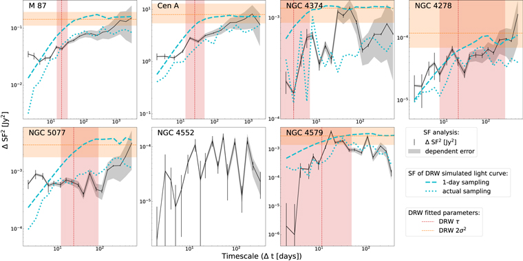
Figure 2. The structure function (SF) analysis result. The error bar shows 1σ uncertainty inferred from the measurement noise variance and the sample numbers. The gray shaded area represents the error caused by the finite number of observations contributing to each bin's measurement. We show the simulated DRW light curve with parameters inferred from Section 3.2's fitting. The cyan dashed line shows the regular sampling of the light curve, while the cyan dotted line shows the actual sampling. The red vertical dashed line indicates the inferred timescale, while the orange horizontal dashed line represents twice the variance, which indicates the expected level of the long-term flux variability for a stationary signal. The comparison of data and simulation suggests that, in our case, the SF may be inadequate for accurately identifying the variability timescale.
Download figure:
Standard image High-resolution imageThe SF provides observations to flux variation between different time lags; therefore, it can reflect the slope properties of the PSD on the short timescale as well as detect the variability saturation on the long timescale. A typical SF is composed of three parts: a flat component in the shortest timescale representing the noise level of the measurement; an increasing trend with a constant slope on a short timescale; and a slope changing to a flat plateau, which reflects the saturation of the variability on a long timescale (see, e.g., Figure 8 in Wielgus et al. 2022). In our SF results, M87, Cen A, and NGC 4374 show an apparent changing slope on the timescale of 10 to 100 days. On the other hand, a suspected steep-to-flat characteristic is detected in NGC 4278's SF, while no detection is found for NGC 5077. The lack of a flat plateau for NGC 4278 and NGC 5077 suggests that there is no stable flux level in their long-term variability, as we can observe in their light curves. With only a few data points (∼20), the SFs of NGC 4552 and NGC 4579 are ambiguous. Therefore, we believe the saturated timescale of a few to 10 days in these cases could be a spurious detection.
The SF has been widely applied in light-curve variability studies (e.g., Collier & Peterson 2001; Czerny et al. 2003; Dexter et al. 2014; Kozłowski 2016a) to avoid ground-based observational bias. It provides a useful insight into the qualitative comparison between sources when the actual PSD is relatively difficult to derive. However, Eracleous et al. (2010) pointed out that the limitation of SF is related to three points. First, properly handling the estimation of the timescale and its uncertainty could be challenging because SF data points are nonindependent. Second, any specific total sampling duration may lead to a spurious saturated timescale. Most important, the SF can still be affected by the observational gap in the light curve.
We further compare the Gaussian process model fitting result (the DRW in the next section) with the SF measurement. We present the SF of a simulated DRW light curve with parameters inferred from the DRW fitting process. In Figure 2, the DRW light curve is labeled in cyan. The dashed line represents the simulated light curve with a regular sampling cadence of 1 day, while the dotted line shows the actual sampling of the SMA observation, and both simulated light curves present the actual duration of the real data. Additionally, we exhibit the DRW-inferred parameters, such as the timescale (vertical red dashed line) and the doubled long-term variance (vertical orange dashed line). The analysis suggests that for M87 and Cen A, the SF (black line) is consistent with the DRW model (cyan dashed line), and the DRW-inferred timescale is situated at the first local maximum, which is generally considered as being where the SF slope breaks. In contrast, the comparison becomes marginally consistent for sources such as NGC 4374 and NGC 4278 and inconsistent for NGC 5077 and NGC 4579. We hypothesize that the SF result is strongly biased by the sampling window effect by simulating the actual sampling DRW light curve (cyan dotted line). Therefore, we conclude that the SF is not sufficient to constrain the timescale for most of the sources.
3.2. The Damped Random Walk Model
To quantify the variable behavior of these sources, we have modeled the light curves as the result of a stochastic DRW process. DRW is a specific Markovian stationary Gaussian process. The application of DRW as a mathematical model to describe the optical variability of quasars was first proposed by Kelly et al. (2009). The validation of DRW to describe the submillimeter light curve of Sgr A* was then investigated by Dexter et al. (2014) and applied to other submillimeter sources by Bower et al. (2015). DRW contains only three parameters: the mean of the light curve μ, the long-term standard deviation σ, and the characteristic timescale τ. The structure function of the DRW model is

The τ determines where the light curve is decorrelated, which corresponds to the saturation of the variability. In the frequency domain, the PSD of the DRW model can be given as
which is composed of a red noise spectrum (αPSD =−2) in the higher-frequency regime (fτ ≫ 1) and a flat white noise spectrum at low frequencies (fτ ≪ 1).
We have followed Kelly et al. (2009) and Dexter et al. (2014) to fit light curves with the following procedure. The likelihood function of a DRW fitting the observed light curve is given by a product of Gaussian describing the residuals from each light-curve point as
where σi
represents measurement uncertainties and  is the difference between each data point and mean,

The quantities Ωi
and  are iterated by the following equations,

and
and regulated by ai , which is the expected correlation between data points,

The iterative procedure starts from the initial conditions

Note that σ2 is the variance of the light curve.
This procedure allows us to calculate the best-fit DRW solution from a given vector of parameters. Therefore, the fit quality can be evaluated by examining the distribution of the residual χ and the reduced chi-square  , calculated as
where ν is the degree of freedom. A proper fit should meet the criteria that the residuals are independent, characterized by a Gaussian distribution with a mean of 0 and a variance of 1, and consequently, the  should approach 1. Figure 3 illustrates the best-fit DRW solution, the light curve, and the residual χ for seven sources. The values of
  are listed in the final column of Table 3. One can observe that the best-fit DRW solution will approach the mean of the light curve if the time interval between two data points is significantly greater than the τ, which agrees with the fitting procedure in Equations (6) and (7). We draw attention to this characteristic of the fitting outcomes, particularly for NGC 4374, since the DRW fits a smaller timescale than the sampling cadence. This results in a DRW light curve with less variability than the actual light curve observed.
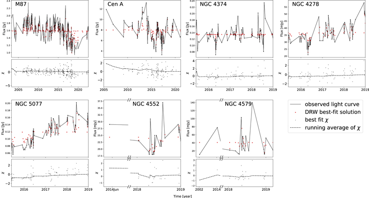
Figure 3. The best-fit DRW solution, the light curve, and the residual χ along with the time. The running average of the residual is also shown for evaluating the distribution of χ.
Download figure:
Standard image High-resolution imageTable 3. Inferred Parameters of DRW Solution
| Source | τ | Δτ | μ | Δμ | σ | Δσ | χ2 |
|---|---|---|---|---|---|---|---|
| (days) | (days) | (Jy) | (Jy) | (Jy) | (Jy) | ||
| M87 | 21 | (15, 32) | 1.589 | (1.530, 1.648) | 0.2676 | (0.2362, 0.3097) | 1.20 |
| Cen A | 26 | (14, 50) | 7.994 | (7.370, 8.677) | 1.9954 | (1.6492, 2.5323) | 1.06 |
| NGC 4278 | 22 | (8, 283) | 0.037 | (0.032, 0.043) | 0.0077 | (0.0059, 0.0209) | 1.06 |
| NGC 4374 | 3.0 | (0.3, 7) | 0.134 | (0.128, 0.141) | 0.0250 | (0.0212, 0.0303) | 1.04 |
| NGC 4552 | ... | (70, ...) | ... | (..., ...) | ... | (..., ...) | 1.12 |
| NGC 4579 | 11.4 | (0.4, 49) | 0.040 | (0.011, 0.073) | 0.0386 | (0.0269, 0.1001) | 1.15 |
| NGC 5077 | 24 | (12, 92) | 0.119 | (0.099, 0.143) | 0.0384 | (0.0300, 0.0683) | 1.07 |
Note. We estimate τ, μ, and σ by calculating the median of the parameter probability distribution and estimating the uncertainty using a 95% CI.
Download table as: ASCIITypeset image
We then applied a Bayesian approach to compute the posterior probability of τ, μ, and σ from the likelihood. Following Dexter et al. (2014), we assume uniform priors on all three parameters. The Metropolis–Hastings algorithm was adopted to sample τ, μ, and σ. The corner plot of the parameters solution is presented in Figure 4 using Cen A as an example. The inferred parameters were estimated by taking the median of the sample population (the red line in Figure 4). We adopted a 2σ uncertainty, which corresponds to the 95% confidence interval (CI) in the population shown in the vertical black dashed line.

Figure 4. Posterior probability distributions of the DRW model parameters using Cen A as an example. The red vertical line displays the median of samples, and the black dashed line labels the 95% CI. Contours correspond to 0.2, 0.5, 0.8, and 0.95 of the posterior volume.
Download figure:
Standard image High-resolution image3.3. Results
We have applied the DRW model to measure the τ of our six new samples and to reanalyze M87. Figure 5 showcases the DRW fit solution of the probability distribution of τ, which is the most relevant parameter in the light curve. A thorough examination of the probability distribution was carried out by plotting the 68%, 95%, and 99.7% CIs for the sample. Note that a good measurement is only valid when both sides of the distribution converge at τ range from τ > Δt and τ < T, where Δt is the minimum observation separation in the light curve, and T is the total light-curve duration. We observe a long tail extending to a short or long timescale, suggesting that τ of the source is not well captured. However, in these cases, the timescale has a high likelihood of being located where the Metropolis–Hastings algorithm conducted intense sampling. As a result, we present the median and 95% CI of the distribution to reflect the highest possible parameter value in these sources.
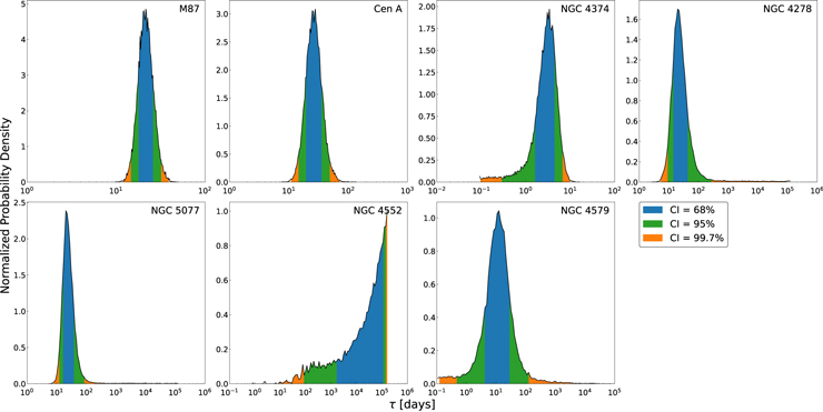
Figure 5. Probability distribution of τ for each source. The 68%, 95%, and 99.7% CIs are labeled in blue, green, and orange, respectively.
Download figure:
Standard image High-resolution imageThe inferred timescale τ, the inferred light-curve mean μ, and the inferred standard distribution σ are presented in Table 3. The reduced χ2 of the best-fit results are calculated in the last column. We note that the correction for the cosmological time dilation is not necessary in these cases. The correction according to Equation (17) in Kelly et al. (2009) is ∼1% for the most distant object NGC 5077 (z ∼ 0.00936; from NASA/IPAC Extragalactic Database), which is smaller than the inferred uncertainty of the timescale.
A long-enough monitoring observation is critical for a DRW study, which provides sufficient probe to the long-term variance, i.e., the white noise part of the PDS. Combining archive data with our monitoring observation, the total light-curve duration for each source is at least 10 times longer than the τ we found, suggesting that the DRW result should be secure in our cases (Kozłowski 2017). On the other hand, the stationary character of the underlying physical process becomes a concern for such a long monitoring observation. In other words, the effect of the underlying process change should be considered.
We found short timescales to be constrained (or with a robust trend to be constrained) in all of our cases except NGC 4552. With a proper sampling cadence (both a cadence much shorter than the timescale and a duration much longer than the timescale), we observed that the degree of how well a timescale can be constrained relies on a certain number of data points. For example, in Dexter et al. (2014), Bower et al. (2015), and this study, sources, such as Sgr A*, M87, M81, and Cen A, whose light curve has over 100 data points, have been accumulated, and this seems to provide a reliable constraint on the timescale. NGC 4374, NGC 4278, and NGC 5077, with only around 80 data points accumulated, exhibit significant uncertainty in either the upper or lower limit. Furthermore, timescale τ becomes poorly constrained in the case of NGC 4579 and NGC4552. Therefore, we suggest that 100 data points seem to be a lower-limit number for measuring a reliable timescale in this experiment. Below we discuss the analysis details for individual cases.
3.3.1. Cen A
We found that the light curve of Cen A can be well described by DRW. A well-constrained τ was measured, while the assessment from both the distribution of residual and reduced χ2 suggests a good fit has been approached. However, we measured that there was roughly a two-time difference in τ when we compared the results of fitting a light curve using linear and logarithmic flux density methods. Except for Cen A, we identify consistent τ in other sources, similar to the result in Dexter et al. (2014). Unlike other data, we suspect that Cen A's flux distribution may show a significant trend to be either a Gaussian or a lognormal distribution (Uttley et al. 2005), and suggests which fit is preferred. We calculated the histogram of the normalized flux of Cen A; however, with limited data, we cannot tell whether Cen A flux follows a Gaussian or lognormal distribution. Here we adopted the linear result of  days, as the linear flux mean and standard deviation are more straightforward.
3.3.2. NGC 4374
We measured  days for NGC 4374 with a good fit quality. A long tail distributed to a short timescale is seen in Figure 5, suggesting that the lower limit of NGC 4374 is not well constrained. The lower-limit long tail reflects the lower limit of 0.3 days for a 95% CI in Table 3. Note that our highest cadence of observation is about 1 day. This result suggests that more daily monitoring observations are necessary for capturing NGC 4374's high-frequency behavior in order to constrain the timescale. The actual timescale is expected to be larger than 3 days since the Metropolis–Hastings algorithm will preferentially sample the long tail of the probability distribution rather than the peak.
3.3.3. NGC 4278 and NGC 5077
We measured  days and
  days for NGC 4278 and NGC 5077, respectively. In both cases, we observed a long tail at the long timescale, suggesting that we do not have a reasonable upper-limit constraint for these sources. They both have χ2 ≈ 1, suggesting a good fit quality. However, the distribution of residuals that have a Gaussian distribution deviates from having a zero mean, suggesting that there is additional noise present in the light curve along with the actual DRW signal. In addition, both sources' light curves show a long-term increase trend and lack of a stable flux level. This evidence suggests that our 4 yr observation did not capture the long-term variable behavior of the sources, but we still detected some short characteristic timescales of the variability. Furthermore, the fit quality suggests that DRW does not describe the light curve well. A model whose PDS slope index is not equal to −2 (e.g., the intraday power spectrum of Sgr A* in Dexter et al. 2014 and the Matern covariance Gaussian process considered by Wielgus et al. 2022) or is a multistochastic Gaussian superposition is possible to consider. Based on current results, weekly or monthly monitoring observations every few years may precisely capture the variability properties.
3.3.4. NGC 4579 and NGC 4552
We have only a small number of data points to marginally constrain the timescale of NGC 4579. Here we adopted a timescale of  days with χ2 = 1.15. The amount of residual is statistically insufficient to provide a robust assessment. In addition, the upper and lower limits are not well constrained, leading to large uncertainty in the inferred τ. For NGC 4552, we cannot constrain any timescale with the current data. Improvement in the numbers of data and flux measurement uncertainty can make a better constraint on timescale measurement in both cases.
3.3.5. M87
We measured a timescale of  days for M87. This measurement is roughly 2 times smaller than the τ in Bower et al. (2015) who measured
  . To investigate the inconsistency in the τ measurement, we separated the light curve into two segments using 2015 as the benchmark. The DRW solution for the before-2015 segment, with a
  and a χ2 ∼ 1, is consistent with Bower et al. (2015); by contrast, the after-2015 segment has a fitting result of
  ,
,  , and
, and  with a χ2 ∼ 1.5. Further, we note that the after-2015 segment is composed of the SMA calibrator database and our observations of the phase calibrator (blue and black marks in Figure 1). By fitting them separately, we found that the after-2015 segment's variability properties are dominated by our observation, while we cannot identify any timescale for the SMA calibrator database. We investigate the systematic difference between these two light curves, and we speculate the variability difference comes from the cadence in which our denser weekly-to-daily observation is advanced to probe the short timescale.
The discrepancy of the fitting result suggests the variability properties vary over these two segments, possibly indicating that an intrinsic physics evolution happens in the historical flux decline, while we have seen a historical low-energy state around 2017–2018 (also see EHT MWL Science Working Group et al. 2021). Nevertheless, the flux decline has recovered itself to the mean flux level in recent observations. We point out that the question of whether the underlying process is stationary on such long timescales is essential to consider in the long-term monitoring study. Here we adopted the result of τ ∼ 20, the whole light-curve measurement, to represent the averaged M87 variability properties.
We noted that M87 shows an extended jet structure in the high-S/N submillimeter observation (large-scale jet lobes on an arcsecond scale; see Figure 1 in Goddi et al. 2021), which we also observed in our M87 snapshot. The core flux can be contaminated by the jet flux in our observation since the angular resolution varies along with the monthly changed configuration schedule. The compact configuration, corresponding to a larger beam size, will naturally include the extended jet component, i.e., the component D in Goddi et al. (2021). This causes an additional artificial variability to be added to the M87 light curve. To remove this artificial variability, we first investigate the variability of the extended jet structure. From a series of high-angular-resolution epochs, we found that component D is relevantly stable with a flux of ∼50 mJy; therefore, we assumed the extended jet structure is static. We note that beam sizes vary from 1'' to 10'' in our observation, and we measured the angular distance between the M87 core and the component D center (here we assumed the flux of component D distributed as an elliptical Gaussian) to be 3 4 from the image in Goddi et al. (2021). We then removed a 50 mJy flux from 66 epochs, whose measurement is considered to include component D based on the beam size and beam position angle. However, the DRW solution of the modified light curve is consistent with the original one, suggesting that DRW is not sensitive to this level of variability in this case.
3.3.6. Limitation and Future Work
The DRW is useful for quantifying the variability properties of the light curves. Moreover, this fitting light-curve method has the advantage of getting rid of observation sampling bias compared to the SF method (Kelly et al. 2009; Dexter et al. 2014). However, it naturally limits itself on the flexibility to probe the light-curve properties in the high-frequency regime, since the use of DRW assumes the PSD slope αPSD = − 2. Several studies have indicated a steeper PSD slope in the optical quasar light curve (Zu et al. 2013; Kasliwal et al. 2015) and The X-ray binary's X-ray variability (Tetarenko et al. 2021). In the context of the Sgr A* submillimeter light curve, the continuous observing mode using ALMA provides a perfect tool to probe the high-frequency regime of the PSD with the use of high-cadence, high-sensitivity light curves and recently found that αPSD is steeper than −2 (Iwata et al. 2020; Murchikova & Witzel 2021; Wielgus et al. 2022). In Wielgus et al. (2022), the SF method reveals a PSD that has a steep slope with αPSD = −2 to −3 that transitions slowly into a white noise on long timescales. Additionally, they apply the Matern covariance model, which is also a Gaussian process model, which provides extra flexibility on fitting the αPSD, and found that αPSD = − 2.6. Compared to the DRW model, the Matern covariance τ measurement is significantly shorter, which may be related to that the DRW can lead to a bias in the τ measurement when the underlying process has αPSD not equal to 2 (Kozłowski 2016b). A potential caveat of our analysis is that our measured τ may have existing bias under the DRW assumption. The use of the Matern covariance in Sgr A* was based on high-quality data; hence, the application of the Matern covariance to our irregular sampling light curve, which, especially, is not sensitive to high frequency, is worth exploring. On the other hand, to better understand the variability of our targets, specifically, the decorrelated timescale and the PSD slope property, both high-cadence, high-S/N light curves and a longer observation span are necessary. The high-frequency PSD slope has the potential to constrain the theoretical accretion model and expand our understanding of Sgr A* and M87 to a population of low-accretion-rate systems.
4. Discussion
4.1. The Black Hole Mass
We have compiled black hole masses from the literature in Table 4. Most of the masses were measured using the multiple dynamical method, which provided a precise mass estimation. By accurately measuring stellar proper motion, Sgr A* has two independent, high-precision measurements with a mass of 4.297 ± 0.012 × 10⁶
M⊙ using the GRAVITY instrument (GRAVITY Collaboration et al. 2022), and a mass of 3.951 ± 0.047 × 10⁶
M⊙ using Keck (Do et al. 2019). We adopted a mass of 4.297 ± 0.012 × 10⁶
M⊙ for Sgr A* and note that, for our purposes, the discrepancy in the mass measurement is irrelevant. We adopted a mass of 6.5 ± 0.7 × 10⁹
M⊙ for M87, which was determined by fitting the physical parameters of lensed emissions near the event horizon (Event Horizon Telescope Collaboration et al. 2019b). This value is consistent with the stellar dynamical method, which suggests a mass of 6.6 ± 0.4 × 10⁹
M⊙ (Gebhardt et al. 2011). M81 has two mass measurements using both the stellar and dynamic methods; therefore, we followed Kormendy & Ho (2013) to adopt a mass of  , which took the mean of two measurements. Cen A has a mass of 5.5 ± 3 × 10⁷
M⊙ using the stellar dynamic method (Cappellari et al. 2009). For NGC 4374, two groups analyzed the same data but identified different black hole masses. We followed Walsh et al. (2010) who clarified this discrepancy and adopted a mass of
, which took the mean of two measurements. Cen A has a mass of 5.5 ± 3 × 10⁷
M⊙ using the stellar dynamic method (Cappellari et al. 2009). For NGC 4374, two groups analyzed the same data but identified different black hole masses. We followed Walsh et al. (2010) who clarified this discrepancy and adopted a mass of  . NGC 5077 has a mass of
  using the gas dynamic method (de Francesco et al. 2008) and NGC 4552 has a mass of (4.7 ± 0.5) × 108 determined by the stellar dynamic method (Sahu et al. 2019). In addition to dynamical methods, we followed the work done by Wang & Zhang (2003) to adopt NGC 4278 and NGC 4579's black hole masses that are estimated by the MBH–σ relationship with a 20% uncertainty on the stellar velocity dispersion. However, we note that systematic errors can be large for all black hole mass estimates.
Table 4. Black Hole Masses Compiled from the Literature
| Source | MBH | Method | References | BH Shadow Size a |
|---|---|---|---|---|
| (M⊙) | (μas) | |||
| Sgr A* | (4.297 ± 0.012) × 106 | Stellar proper motion | GRAVITY Collaboration et al. (2022) | ∼51.3 |
| M87 | (6.5 ± 0.7) × 109 | Lensed emission | Event Horizon Telescope Collaboration et al. (2019b) | ∼38.2 |
| M81 |

| Stellar and gas | Kormendy & Ho (2013) | ∼1.8 |
| Cen A | (5.5 ± 3) × 107 | Stellar | Neumayer (2010) | ∼1.4 |
| NGC 4278 | (3.1 ± 0.5) × 108 | M–σ relation | Wang & Zhang (2003) | ∼1.8 |
| NGC 4374 |

| Gas | Walsh et al. (2010) | ∼5.0 |
| NGC 4552 | (4.7 ± 0.5) × 108 | Stellar | Sahu et al. (2019) | ∼2.8 |
| NGC 4579 | (1.1 ± 0.2) × 108 | M–σ relation | Wang & Zhang (2003) | ∼0.6 |
| NGC 5077 |

| Gas | de Francesco et al. (2008) | ∼1.5 |
Note.
a We assume a fiducial radius of 5Rs for the potential observable black hole shadow size. The angular diameter of the black hole shadow is calculated using 5Rs = 10GM/Dc2, where D is the distance to the observer. The distances of the black holes are adopted from Sgr A*: GRAVITY Collaboration et al. (2022); M87: Event Horizon Telescope Collaboration et al. (2019b); M81: Freedman et al. (1994); Cen A: Harris et al. (2010); and others from NASA/IPAC Extragalactic Database (NED).Download table as: ASCIITypeset image
4.2. MBH versus τ
To qualitatively understand the physical meaning of the timescale and the connection with the black hole mass, we presented the black hole mass–characteristic timescale correlation among nine sources in Figure 6. New LLAGN samples in this study are labeled in purple, while sources measured in previous studies are labeled in different colors. Here we compare these measured timescales with the physical timescales in the accretion system. The orbital timescale torb and the viscous timescale tvisc, which scale with the black hole mass MBH and Schwarzschild radius Rs , can be expressed in the following equations:
The use of parameter α ∼ 0.03 − 0.05 and the scale height H/R ∼ 0.6 is based on previous simulation results (Narayan et al. 2012).
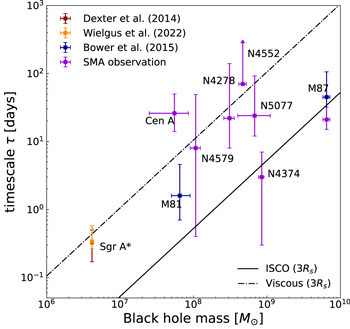
Figure 6. MBH–τ relationship. We present the DRW-inferred τ vs. MBH for our six new sources (labeled in purple), the reanalyzed result of M87 (also labeled in purple), and other sources (labeled as different colors according to the provenance) from previous studies.
Download figure:
Standard image High-resolution imageTwo physical timescales are labeled in Figure 6 with the innermost stable circular orbit (ISCO) radius (3Rs = 6GM/c2) for a Schwarzschild black hole. We found that no source falls under the orbital ISCO timescale, and most sources have a characteristic timescale comparable with the orbital or viscous timescale in the inner region of the accretion disk. Note that the new M87 result agrees with the orbital ISCO timescale since the period of ISCO varies from 5 days to about a month, relevant to the spin of the black hole from 1 to 0. NGC 4374 is situated near the orbital ISCO line. However, as previously discussed in the analysis section, the algorithm has a tendency to choose the unconstrained long tail. As a result, we anticipate that the well-constrained timescale would be larger.
Bower et al. (2015) found a linear MBH–τ correlation among three LLAGNs, Sgr A*, M81, and M87. Our new results agree with the trend they found. Besides the lower-limit measurement for NGC 4552, the whole samples show a significant trend that the timescale of these sources increases along with their black hole mass. This can be understood by approximating the timescale scaling around the black hole to be  (a simplification of Equations (11) and (12)). One can expect a linear black hole mass–minimum timescale correlation to establish when the emission originates from the same Rs
, where Rs
is in the event horizon scale. In contrast, Cen A shows a much larger timescale in this population and deviates from the linear relationship. The VLBI experiment result (discussed in the next paragraph) suggests that our timescale of a few to 10 days of Cen A comes from a more outer region of the accretion disk. From our result, the black hole mass–minimum timescale correlation in the submillimeter light curve indicates that the submillimeter emission originates from the event horizon scale for these sources.
(a simplification of Equations (11) and (12)). One can expect a linear black hole mass–minimum timescale correlation to establish when the emission originates from the same Rs
, where Rs
is in the event horizon scale. In contrast, Cen A shows a much larger timescale in this population and deviates from the linear relationship. The VLBI experiment result (discussed in the next paragraph) suggests that our timescale of a few to 10 days of Cen A comes from a more outer region of the accretion disk. From our result, the black hole mass–minimum timescale correlation in the submillimeter light curve indicates that the submillimeter emission originates from the event horizon scale for these sources.
This interpretation is consistent with our understanding of the VLBI experiment results and the multiwavelength studies. The synchrotron radiation dominates the emission that originates from the accretion flow at the black hole vicinity, and the synchrotron self-absorption leads to an optically thick photosphere that shrinks along with the frequency until the spectral peak. For instance, we saw the intrinsic size of the emission core shrink along with the higher-frequency VLBI observation for M87 and Sgr A* (Hada et al. 2011; Johnson et al. 2018). The black hole image was then resolved by the EHT in the 2017 campaign using the 230 GHz global VLBI. The sizes of the rings are ∼5.5Rs and ∼4Rs , respectively (Event Horizon Telescope Collaboration et al. 2019a; Event Horizon Telescope Collaboration et al. 2022a). By contrast, an edge-brightened jet structure was observed in the 2017 EHT campaign for Cen A, and the interpreted core size is ∼32μas (∼120Rs ; Janssen et al. 2021). Based on the jet model, the optically thin frequency is expected to be located between the wavelengths from terahertz to far-infrared and further, as agreed by the Cen A core SED study (Abdo et al. 2010). In the cases of M81 and NGC 4374, Jiang et al. (2018) and Jiang et al. (2021) report the unresolved core observation with VLBA at 88 GHz. Combined with their flat-to-inverse slope spectrum, the VLBI measurement suggests the upper limit of the core size at 230 GHz to be <80Rs and <30Rs for M81 and NGC 4374. On the other hand, the submillimeter emission core size of NGC 4278, NGC 4579, and NGC 5077, lacking a high-angular-resolution observation, is unknown. However, one can interpret that the submillimeter emission is optically thin for NGC 4278 and NGC 4579 from their SED study (see Mason et al. 2013; Bandyopadhyay et al. 2019). Although the SED study is incomplete, it generally provides properties of the nonthermal emission and further supports our timescale result.
4.3. MBH–τ Scaling Relation
To investigate the MBH–τ scaling relationship suggested in Figure 6, we perform both linear and power fits on our sample set. This sample set includes τ values from Sgr A* and M81 obtained from the literature and excludes the lower-limit constraint of NGC 4552. We exclude Cen A from our analysis of the mass scaling relationship because its submillimeter properties, as suggested by VLBI experiments and SED studies, differ from those of our other samples. When multiple timescale measurements are available, we use the best measurement for our discussion of the mass scaling relationship. For Sgr A*, we adopt the 8 hr measurement reported in Wielgus et al. (2022), as it provides high-quality data that were previously unattainable. Additionally, it is worth mentioning that Wielgus et al. (2022) have extensively discussed the comparison of timescale measurements obtained from different sets of light curves, which indicates the evolution of the physical state of Sgr A*. For M87, we use our 21 day measurement, as it provides the densest sampling cadence and longest time baseline in our observation.
Following Kelly (2007), we adopt a Bayesian method and apply a Metropolis–Hastings sampler to account for both MBH and τ uncertainties in the linear regression process in both linear space and logarithmic space. The best-fit parameters, i.e., the slope and the intercept, are estimated from the median of the probability distribution, and we present 1σ as the fit uncertainty.
One can expect a τ–MBH linear relationship ( ) from the physical interpretation. However, we found a linear fit result of
  with a coefficient of determination of R2 ∼ 0.23, suggesting that the relationship between τ and MBH is not simply linear. On the other hand, the power-law fit provides a result of
with a coefficient of determination of R2 ∼ 0.61, and we report a 1σ intrinsic scatter of  dex for the data.
Based on our limited sample, our experiment suggests that there is a scaling relationship between the black hole mass and timescale; however, the correlation is weak and there is significant intrinsic scatter, implying that there may be a third parameter involved that may not be easy to measure, such as the optical depth. We highlight that this relationship is largely driven by Sgr A* and M87. By considering different measurements that reflect the different status of the sources' underlying physics for Sgr A* and M87, we found that the relationship can appear more steep or more shallow and tighter or looser. This evidence suggests that the robustness of the relationship requires further samples to be added to the MBH–τ correlation, especially the timescale measurement for black hole mass equal to or smaller than Sgr A*, and black hole mass larger than M87.
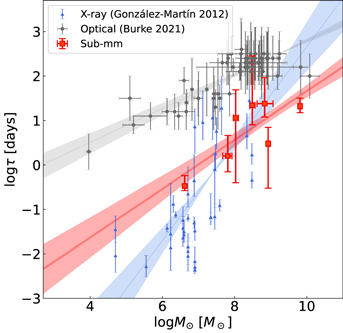
In Figure 7, we present the linear regression result of our submillimeter measurement as well as the optical and X-ray linear fit from Burke et al. (2021) and González-Martín & Vaughan (2012). The optical data, containing 67 AGNs, have the best-fit model of  , which considers errors in both parameters. X-ray data, including 42 light-curve measurements, suggest a linear correlation fit of
  , but without considering the black hole mass error.
Figure 7. MBH–τ correlation in submillimeter vs. optical vs. X-ray. Different shapes and colors of marks label data from the different wavelengths. Solid lines represent the linear regression result from each group of data. The shaded area displays the fitting uncertainty in one σ level. Note that for submillimeter, the results presented exclude the case of Cen A.
Download figure:
Standard image High-resolution image
While various types of AGNs may be classified into different accretion models, such as the standard thin disk model and the radiatively inefficient accretion flow, resulting in different wavelengths being attributed to various emission mechanisms, a comparison of variability properties between wavelengths still offers a unique opportunity to gain insight into the disk configuration and the origin of variability. The submillimeter and X-ray wavelengths show a significantly shorter timescale compared to the optical wavelength, suggesting that submillimeter and X-ray variability can provide information about the inner regions of the black hole system. On the other hand, the optical timescale is comparable to that of the outer disk's dynamics or thermal timescale. These observations of the timescales at different wavelengths are in agreement with our current understanding of the structure of the accretion disk/flow. Moreover, slopes are different in the X-ray, submillimeter, and optical MBH–τ correlations, which come with 1, 0.6, and 0.4, respectively. In the inner part of the accretion flow, X-ray correlation indicates that plasma around the black hole (corona) correlates tightly with black hole mass. In contrast to X-ray, our submillimeter correlation may be impacted by additional physical parameters, such as the optical depth or black hole spin. The optical correlation in the outer region suggests that other factors have a significant impact on the variability or that the variability origin differs from that seen in the X-ray or submillimeter data. However, it is important to note that the X-ray sample shows more scatter than the optical and submillimeter samples, which was attributed to the absorption along the line of sight proposed by González-Martín (2018), indicating a more complex situation. Meanwhile, the submillimeter results are less scattered but remain uncertain due to being based on a smaller population.
5. Conclusion
In this study, we investigate the variability of seven LLAGNs' submillimeter light curves. All sources are variable at levels ranging from ∼10% to ∼100%. We show that submillimeter light curves can be well described using the DRW model and we determine the characteristic timescales of the variability. The LLAGNs' timescales are then found to have a correlation with their black hole masses. This correlation suggests that the accretion flow at the submillimeter wavelength is transparent down to the event horizon scale, and indicates that accretion disk size may scale with black hole mass in a low-accretion system. This method, by measuring timescales, provides an independent way to test the black hole size. Moreover, this variability study provides an important identification of potential EHT targets. These sources with their black hole masses and distances to Earth suggest a few microarcsecond black hole shadow sizes, which may be resolvable by using the EHT at a higher frequency (345 or 690 GHz; see Doeleman et al. 2019) or with the space VLBI (e.g., Fish et al. 2020; Roelofs et al. 2021; Gurvits et al. 2022).
Acknowledgments
We thank the anonymous referees for helpful comments that improved the paper. We appreciate the support of this work from the Ministry of Science and Technology (MOST) of Taiwan (code: 110-2923-M-001-001-) and the National Science and Technology Council (NSTC) of Taiwan (code: 111-2124-M-001-005-). The Submillimeter Array is a joint project between the Smithsonian Astrophysical Observatory and the Academia Sinica Institute of Astronomy and Astrophysics and is funded by the Smithsonian Institution and the Academia Sinica. We recognize that Maunakea is a culturally important site for the indigenous Hawaiian people; we are privileged to study the cosmos from its summit. This paper makes use of the following ALMA data: ADS/JAO.ALMA # 2011.0.00010.S, ADS/JAO.ALMA # 2012.1.00019.S, ADS/JAO.ALMA # 2012.1.00139.S, ADS/JAO.ALMA # 2013.1.00803.S, ADS/JAO.ALMA # 2013.1.01342.S, ADS/JAO.ALMA # 2015.1.00483.S, ADS/JAO.ALMA # 2015.1.01577.S, ADS/JAO.ALMA # 2017.1.00090.S, ADS/JAO.ALMA # 2017.1.00886.L, and ADS/JAO.ALMA # 2018.A.00062.S. ALMA is a partnership of ESO (representing its member states), NSF (USA), and NINS (Japan), together with NRC (Canada), MOST and ASIAA (Taiwan), and KASI (Republic of Korea), in cooperation with the Republic of Chile. The Joint ALMA Observatory is operated by ESO, AUI/NRAO, and NAOJ.
Facilities: SMA - SubMillimeter Array, ALMA - Atacama Large Millimeter Array, IRAM:Interferometer.
Software: MIR-IDL, Miriad, CASA.