


Abstract
Several publications highlight the importance of the observations of bow shocks to learn more about the surrounding interstellar medium and radiation field. We revisit the most prominent dusty and gaseous bow shock source, X7, close to the supermassive black hole, Sgr A*, using multiwavelength analysis. For the purpose of this study, we use Spectrograph for Integral Field Observations in the Near Infrared (SINFONI) (H+K-band) and NACO L'- and M'-band) data sets between 2002 and 2018 with additional COMIC/ADONIS+RASOIR (L'-band)7data of 1999. By analyzing the line maps of SINFONI, we identify a velocity of ∼200 km s−1 from the tip to the tail. Furthermore, a combination of the multiwavelength data of NACO and SINFONI in the H-, K-, L'-, and M'-bands results in a two-component blackbody fit that implies that X7 is a dust-enshrouded stellar object. The observed ongoing elongation and orientation of X7 in the Brγ line maps and the NACO L'-band continuum indicate a wind arising at the position of Sgr A* or at the IRS16 complex. Observations after 2010 show that the dust and the gas shell seems to be decoupled in the projection from its stellar source S50. The data also implies that the tail of X7 thermally heats up due to the presence of S50. The gas emission at the tip is excited because of the related forward scattering (Mie scattering), which will continue to influence the shape of X7 in the near future. In addition, we find excited [Fe iii] lines, which together with the recently analyzed dusty sources and the Brγ-bar underline the uniqueness of this source.
Export citation and abstract BibTeX RIS
1. Introduction
The prominent variable radio source Sgr A* is located in the center of our galaxy (Balick & Brown 1974). This source emits across a broad range of wavelengths, ranging from the radio up to the X-ray domain, with the peak at submillimeter wavelengths (see, e.g., Genzel et al. 2010; Eckart et al. 2017, and references therein). Although Sgr A* is a low-luminosity source, its monitoring has been of high interest because of order-of-magnitude flares in the near-infrared (NIR) and X-ray domains (Witzel et al. 2012; Do et al. 2019). Because of its nonthermal radiative properties, compact nature, variability, and position at the Galactic center (GC), it has been associated with a supermassive black hole (SMBH) since its discovery (Lynden-Bell & Rees 1971), with most of the alternatives being ruled out based on the current observational data (Eckart et al. 2017).
Sgr A* is also the only SMBH to date, where we can detect and monitor orbiting stars. Some of them are located inside the S-cluster, hence, they are called S-stars. These stars show pericenter distances of several hundred astronomical units (Gillessen et al. 2009; Parsa et al. 2017; Ali et al. 2020). Recently discovered stars push this distance an order of magnitude closer to the SMBH (Peißker et al. 2020a, 2020d). These S-stars have been widely covered by many publications. For example, Eckart & Genzel (1996) derived from the stellar proper motion a direct mass estimate of Sgr A*. In addition, Ghez et al. (2002) and Eckart et al. (2002) found stellar accelerations based on the orbital curvature. Genzel et al. (2000) derived a velocity dispersion as a function of the distance of S-stars and found values of up to several hundred kilometers per second.
One of the controversial but also interesting sources in the field of view (FOV) is the GC gas cloud G2 (Gillessen et al. 2012; Eckart et al. 2013; Valencia-S. et al. 2015; Shahzamanian et al. 2017; Zajaček et al. 2017; Peißker et al. 2020b) also known as the Dusty S-cluster Object (DSO). 8 This object was found on its way to approaching Sgr A* in the Doppler-shifted Brγ maps of the Spectrograph for Integral Field Observations in the Near Infrared (SINFONI), an NIR instrument mounted at the Very Large Telescope (VLT; Chile/Paranal). In combination with the observed dust emission in the L'-band (3.8 μm) with NACO (also operating in the NIR, mounted at the VLT), the authors of Gillessen et al. (2012, 2013) and Pfuhl et al. (2015) have claimed that the object will get disrupted during or after its periapse passage. Later on, Plewa et al. (2017) stated that the density of the ambient medium of Sgr A* is too low to cause a disruptive event. Even more, they excluded the possibility of a drag force acting on the DSO. In contrast, Gillessen et al. (2019) reported a drag force that influenced the observed Doppler-shifted Brγ line shape. This underlines the ongoing confusion about the nature of the source. However, in Peißker et al. (2020b) we presented a spectral energy distribution (SED) derived from the H-, K-, and L'-band data of NACO and SINFONI. This SED consists of a dusty and stellar component and shows that the DSO is more likely a Young Stellar Object instead of a coreless ∼3 × M⊕ cloud that moves on a Keplerian orbit around a 4.1 × 10⁶ M⊙ SMBH.
Clénet et al. (2003) and Clénet et al. (2005) reported for the first time two comet-shaped sources, namely, X3 and X7. These dusty objects can be found in the mid-infrared (MIR) but also show an NIR counterpart. Because of its close projected distance to X7, another line emitting source is located, which we call X7.1 (G5 in Ciurlo et al. 2020).
The identification of these objects is still challenging, which is illustrated in Figure 1 in Peißker et al. (2020b). The potentially temporary distance of X7 and X7.1/G5 can lead to confusion about the identification without spectroscopic analysis. It is, for instance, not clear why the dusty object X7.1/G5 with an approximate L-band magnitude of 14.11 mag (∼0.57 mJy) can neither be observed in the NACO (L'-band) data presented in this work nor in the 3.8 μm continuum data shown in Ciurlo et al. (2020) (see the extended data in Figure 2 in the related publication). A dust-enshrouded source with a stellar counterpart should be detectable in the L'-band as presented in Peißker et al. (2020b). A reliable approach is the spectroscopic analysis in combination with multiwavelength observations. This underlines the need for broad observation programs. Following the example of the DSO and X7.1, we emphasize a multiwavelength analysis of these (potentially) dust-enshrouded stars. With the observational coverage of different bands in combination with spectroscopy, the confusion about the nature of these objects can be minimized (see Zajaček et al. 2017).
However, Mužić et al. (2010) analyzed the X7 source in detail and showed a connection to a possible nuclear wind that arises at the position of Sgr A*. This wind is also mentioned in several observational and theoretical publications (Mužić et al. 2007; Zajaček et al. 2016; Yusef-Zadeh et al. 2017b; Peißker et al. 2020b, 2020c; Yusef-Zadeh et al. 2020). In this regard, Peißker et al. (2019) reported a new bow shock source in the central arcseconds that the authors call X8 (G6 in Ciurlo et al. 2020) because of its close projected distance to X7. These two objects are the closest bow shock sources that could be used to determine the properties of a possible wind that arises at the position of Sgr A*.
In this work, we update the analysis of X7 done by Mužić et al. (2007, 2010) with the help of SINFONI integral field spectroscopy and NACO continuum data that cover almost 16 years. Additionally, we use L'-band continuum COMIC/ADONIS+RASOIR data of 1999 to extend the analysis of X7 to about 20 years. This work is part of a broader investigation that is divided into two publications. Here, we emphasize the observational results and give an outlook on the second part where we theoretically investigate the observed source X7. In the second part of this survey, we will apply two models to describe an open and closed bow shock based on the work of Wilkin (1996, 2000) and Christie et al. (2016). The spectroscopic capabilities of SINFONI give us access to investigate the velocity along the bow shock source that could help to describe the nuclear and the stellar-wind interaction as well as prominent Doppler-shifted emission lines. Furthermore, we investigate the close projected distance of S50 to X7. This S-cluster star can be associated with the stellar counterpart of X7 and seems to interact with the dust tail of the bow shock source. In the multiwavelength analysis, we also model a two-component SED of X7. We also witness ongoing decoupling in the projection of the dusty and gaseous shell of S50 that is associated with X7.
In the following Section 2, we introduce the instruments used and the analytical techniques. The results of the analysis are presented in Section 3. Section 4 summarizes the results and provides an outlook for future observations. In Appendix A, we provide some supplementary information regarding the analysis and a possible scenario. In addition, we list the SINFONI and NACO data that were used for the analysis.
2. Data and Analysis
In this section, we give a brief overview about the instruments used, the data reduction, and the applied analysis tools.
2.1. SINFONI and NACO
The SINFONI was mounted on the VLT and underwent an upgrade (for further information about the upgrade, see Kuntschner et al. 2014; Marchetti et al. 2014; Pearson et al. 2016). SINFONI operates in the NIR and provides observations in the J- (1.10–1.40 μm), H- (1.45–1.85 μm), K- (1.95–2.45 μm), and H + K-bands (1.45–2.45 μm). The output files of the ESO pipeline are in the shape of a three-dimensional data cube. This data cube consists of two spatial dimensions and one spectral dimension. The components of the data cubes are described in spaxels (pixels containing a spectrum, see Hörtner et al. 2012) rather than pixels. With SINFONI, we are able to isolate single emission lines in the H + K-band to create channel (line) maps. In comparison, the NACO 9 instrument works also in the J, L', and M'-bands (Lenzen et al. 2003; Rousset et al. 2003). Since dust can be traced in higher wavelengths, the L'-band setup of NACO is favored for the search of the dusty bow shock source. In both cases, we apply the usual data reduction steps, e.g., dark- and flat-field corrections. We also apply the mandatory sky correction to the adaptive optics (AO) corrected data. Additional correction steps are described in detail in Peißker et al. (2019, 2020a, 2020b, 2020c, 2020d) where the data analyzed here is also used. See Tables 1, 2, 3, 4, 5, 6 and 7, and Appendix E for a detailed overview about the data used.
Table 1. SINFONI Data of 2005, 2006, 2007, 2008, and 2009
| Date | Observation ID | Amount of on Source Exposures | Exposure Time | ||
|---|---|---|---|---|---|
| Total | Medium | High | (s) | ||
| 2005 Jun 16 | 075.B-0547(B) | 20 | 12 | 8 | 300 |
| 2005 Jun 18 | 075.B-0547(B) | 21 | 2 | 19 | 60 |
| 2006 Mar 17 | 076.B-0259(B) | 5 | 0 | 3 | 600 |
| 2006 Mar 20 | 076.B-0259(B) | 1 | 1 | 0 | 600 |
| 2006 Mar 21 | 076.B-0259(B) | 2 | 2 | 0 | 600 |
| 2006 Apr 22 | 077.B-0503(B) | 1 | 0 | 0 | 600 |
| 2006 Aug 17 | 077.B-0503(C) | 1 | 0 | 1 | 600 |
| 2006 Aug 18 | 077.B-0503(C) | 5 | 0 | 5 | 600 |
| 2006 Sep 15 | 077.B-0503(C) | 3 | 0 | 3 | 600 |
| 2007 Mar 26 | 078.B-0520(A) | 8 | 1 | 2 | 600 |
| 2007 Apr 22 | 179.B-0261(F) | 7 | 2 | 1 | 600 |
| 2007 Apr 23 | 179.B-0261(F) | 10 | 0 | 0 | 600 |
| 2007 Jul 22 | 179.B-0261(F) | 3 | 0 | 2 | 600 |
| 2007 Jul 24 | 179.B-0261(Z) | 7 | 0 | 7 | 600 |
| 2007 Sep 3 | 179.B-0261(K) | 11 | 1 | 5 | 600 |
| 2007 Sep 4 | 179.B-0261(K) | 9 | 0 | 0 | 600 |
| 2008 Apr 6 | 081.B-0568(A) | 16 | 0 | 15 | 600 |
| 2008 Apr 7 | 081.B-0568(A) | 4 | 0 | 4 | 600 |
| 2009 May 21 | 183.B-0100(B) | 7 | 0 | 7 | 600 |
| 2009 May 22 | 183.B-0100(B) | 4 | 0 | 4 | 400 |
| 2009 May 23 | 183.B-0100(B) | 2 | 0 | 2 | 400 |
| 2009 May 24 | 183.B-0100(B) | 3 | 0 | 3 | 600 |
Note. The total amount of data is listed.
Download table as: ASCIITypeset image
Table 2. SINFONI Data of 2010, 2011, 2012, and 2013
| Date | Observation ID | Amount of on Source Exposures | Exposure Time | ||
|---|---|---|---|---|---|
| Total | Medium | High | (s) | ||
| 2010 May 10 | 183.B-0100(O) | 3 | 0 | 3 | 600 |
| 2010 May 11 | 183.B-0100(O) | 5 | 0 | 5 | 600 |
| 2010 May 12 | 183.B-0100(O) | 13 | 0 | 13 | 600 |
| 2011 Apr 11 | 087.B-0117(I) | 3 | 0 | 3 | 600 |
| 2011 Apr 27 | 087.B-0117(I) | 10 | 1 | 9 | 600 |
| 2011 May 02 | 087.B-0117(I) | 6 | 0 | 6 | 600 |
| 2011 May 14 | 087.B-0117(I) | 2 | 0 | 2 | 600 |
| 2011 Jul 27 | 087.B-0117(J)/087.A-0081(B) | 2 | 1 | 1 | 600 |
| 2012 Mar 18 | 288.B-5040(A) | 2 | 0 | 2 | 600 |
| 2012 May 05 | 087.B-0117(J) | 3 | 0 | 3 | 600 |
| 2012 May 20 | 087.B-0117(J) | 1 | 0 | 1 | 600 |
| 2012 Jun 30 | 288.B-5040(A) | 12 | 0 | 10 | 600 |
| 2012 Jul 01 | 288.B-5040(A) | 4 | 0 | 4 | 600 |
| 2012 Jul 08 | 288.B-5040(A)/089.B-0162(I) | 13 | 3 | 8 | 600 |
| 2012 Sep 08 | 087.B-0117(J) | 2 | 1 | 1 | 600 |
| 2012 Sep 14 | 087.B-0117(J) | 2 | 0 | 2 | 600 |
| 2013 Apr 05 | 091.B-0088(A) | 2 | 0 | 2 | 600 |
| 2013 Apr 06 | 091.B-0088(A) | 8 | 0 | 8 | 600 |
| 2013 Apr 07 | 091.B-0088(A) | 3 | 0 | 3 | 600 |
| 2013 Apr 08 | 091.B-0088(A) | 9 | 0 | 6 | 600 |
| 2013 Apr 09 | 091.B-0088(A) | 8 | 1 | 7 | 600 |
| 2013 Apr 10 | 091.B-0088(A) | 3 | 0 | 3 | 600 |
| 2013 Aug 28 | 091.B-0088(B) | 10 | 1 | 6 | 600 |
| 2013 Aug 29 | 091.B-0088(B) | 7 | 2 | 4 | 600 |
| 2013 Aug 30 | 091.B-0088(B) | 4 | 2 | 0 | 600 |
| 2013 Aug 31 | 091.B-0088(B) | 6 | 0 | 4 | 600 |
| 2013 Sep 23 | 091.B-0086(A) | 6 | 0 | 0 | 600 |
| 2013 Sep 25 | 091.B-0086(A) | 2 | 1 | 0 | 600 |
| 2013 Sep 26 | 091.B-0086(A) | 3 | 1 | 1 | 600 |
Download table as: ASCIITypeset image
Table 3. SINFONI Data of 2014 and 2015
| Date | Observation ID | Amount of on Source Exposures | Exposure Time | ||
|---|---|---|---|---|---|
| Total | Medium | High | (s) | ||
| 2014 Feb 27 | 092.B-0920(A) | 4 | 1 | 3 | 600 |
| 2014 Feb 28 | 091.B-0183(H) | 7 | 3 | 1 | 400 |
| 2014 Mar 01 | 091.B-0183(H) | 11 | 2 | 4 | 400 |
| 2014 Mar 02 | 091.B-0183(H) | 3 | 0 | 0 | 400 |
| 2014 Mar 11 | 092.B-0920(A) | 11 | 2 | 9 | 400 |
| 2014 Mar 12 | 092.B-0920(A) | 13 | 8 | 5 | 400 |
| 2014 Mar 26 | 092.B-0009(C) | 9 | 3 | 5 | 400 |
| 2014 Mar 27 | 092.B-0009(C) | 18 | 7 | 5 | 400 |
| 2014 Apr 02 | 093.B-0932(A) | 18 | 6 | 1 | 400 |
| 2014 Apr 03 | 093.B-0932(A) | 18 | 1 | 17 | 400 |
| 2014 Apr 04 | 093.B-0932(B) | 21 | 1 | 20 | 400 |
| 2014 Apr 06 | 093.B-0092(A) | 5 | 2 | 3 | 400 |
| 2014 Apr 08 | 093.B-0218(A) | 5 | 1 | 0 | 600 |
| 2014 Apr 09 | 093.B-0218(A) | 6 | 0 | 6 | 600 |
| 2014 Apr 10 | 093.B-0218(A) | 14 | 4 | 10 | 600 |
| 2014 May 08 | 093.B-0217(F) | 14 | 0 | 14 | 600 |
| 2014 May 09 | 093.B-0218(D) | 18 | 3 | 13 | 600 |
| 2014 Jun 09 | 093.B-0092(E) | 14 | 3 | 0 | 400 |
| 2014 Jun 10 | 092.B-0398(A)/093.B-0092(E) | 5 | 4 | 0 | 400/600 |
| 2014 Jul 08 | 092.B-0398(A) | 6 | 1 | 3 | 600 |
| 2014 Jul 13 | 092.B-0398(A) | 4 | 0 | 2 | 600 |
| 2014 Jul 18 | 092.B-0398(A)/093.B-0218(D) | 1 | 0 | 0 | 600 |
| 2014 Aug 18 | 093.B-0218(D) | 2 | 0 | 1 | 600 |
| 2014 Aug 26 | 093.B-0092(G) | 4 | 3 | 0 | 400 |
| 2014 Aug 31 | 093.B-0218(B) | 6 | 3 | 1 | 600 |
| 2014 Sep 07 | 093.B-0092(F) | 2 | 0 | 0 | 400 |
| 2015 Apr 12 | 095.B-0036(A) | 18 | 2 | 0 | 400 |
| 2015 Apr 13 | 095.B-0036(A) | 13 | 7 | 0 | 400 |
| 2015 Apr 14 | 095.B-0036(A) | 5 | 1 | 0 | 400 |
| 2015 Apr 15 | 095.B-0036(A) | 23 | 13 | 10 | 400 |
| 2015 Aug 01 | 095.B-0036(C) | 23 | 7 | 8 | 400 |
| 2015 Sep 05 | 095.B-0036(D) 17 | 11 | 4 | 400 | |
Download table as: ASCIITypeset image
Table 4. SINFONI Data of 2016
| Date | Observation ID | Amount of on Source Exposures | Exp. Time | ||
|---|---|---|---|---|---|
| Total | Medium | High | (s) | ||
| 2016 Mar 15 | 096.B-0157(B) | 15 | 0 | 15 | 400 |
| 2016 Mar 16 | 096.B-0157(B) | 17 | 0 | 17 | 400 |
| 2016 Apr 14 | 594.B-0498(R) | 12 | 0 | 12 | 400 |
| 2016 Apr 16 | 594.B-0498(R) | 10 | 0 | 8 | 600 |
| 2016 Jul 09 | 097.B-0050(A) | 15 | 0 | 2 | 600 |
| 2016 Jul 11 | 097.B-0050(A) | 38 | 0 | 3 | 600 |
| 2016 Jul 12 | 097.B-0050(A) | 27 | 0 | 13 | 600 |
Download table as: ASCIITypeset image
Table 5. SINFONI Data of 2017
| Date | Observation ID | Amount of on Source Exposures | Exposure Time | ||
|---|---|---|---|---|---|
| Total | Medium | High | (s) | ||
| 2017 Mar 15 | 598.B-0043(D) | 5 | 2 | 0 | 600 |
| 2017 Mar 19 | 598.B-0043(D) | 11 | 0 | 5 | 600 |
| 2017 Mar 20 | 598.B-0043(D) | 15 | 4 | 11 | 600 |
| 2017 Mar 21 | 598.B-0043(D) | 1 | 0 | 0 | 600 |
| 2017 May 20 | 0101.B-0195(B) | 8 | 2 | 6 | 600 |
| 2017 Jun 01 | 598.B-0043(E) | 5 | 0 | 3 | 600 |
| 2017 Jun 02 | 598.B-0043(E) | 8 | 0 | 8 | 600 |
| 2017 Jun 29 | 598.B-0043(E) | 4 | 2 | 17 | 600 |
| 2017 Jul 20 | 0101.B-0195(C) | 8 | 5 | 0 | 600 |
| 2017 Jul 28 | 0101.B-0195(C) | 6 | 0 | 0 | 600 |
| 2017 Jul 29 | 0101.B-0195(D) | 9 | 0 | 0 | 600 |
| 2017 Aug 01 | 0101.B-0195(E) | 4 | 0 | 0 | 600 |
| 2017 Aug 19 | 598.B-0043(F) | 8 | 0 | 2 | 600 |
| 2017 Sep 13 | 598.B-0043(F) | 8 | 0 | 0 | 600 |
| 2017 Sep 15 | 598.B-0043(F) | 10 | 1 | 1 | 600 |
| 2017 Sep 29 | 598.B-0043(F) | 2 | 0 | 0 | 600 |
| 2017 Oct 15 | 0101.B-0195(F) | 2 | 0 | 0 | 600 |
| 2017 Oct 17 | 0101.B-0195(F) | 4 | 0 | 0 | 600 |
| 2017 Oct 23 | 598.B-0043(G) | 3 | 0 | 0 | 600 |
Download table as: ASCIITypeset image
Table 6. K-band Data Observed with NACO between 2002 and 2018
| NACO | ||||
|---|---|---|---|---|
| Date | Observation ID | Number of Exposures | Total Exposure Time | λ |
| (s) | ||||
| 2002 Jul 31 | 60.A-9026(A) | 61 | 915 | K |
| 2003 Jun 13 | 713-0078(A) | 253 | 276.64 | K |
| 2004 Jul 06 | 073.B-0775(A) | 344 | 308.04 | K |
| 2004 Jul 08 | 073.B-0775(A) | 285 | 255.82 | K |
| 2005 Jul 25 | 271.B-5019(A) | 330 | 343.76 | K |
| 2005 Jul 27 | 075.B-0093(C) | 158 | 291.09 | K |
| 2005 Jul 29 | 075.B-0093(C) | 101 | 151.74 | K |
| 2005 Jul 30 | 075.B-0093(C) | 187 | 254.07 | K |
| 2005 Jul 30 | 075.B-0093(C) | 266 | 468.50 | K |
| 2005 Aug 02 | 075.B-0093(C) | 80 | 155.77 | K |
| 2006 Aug 02 | 077.B-0014(D) | 48 | 55.36 | K |
| 2006 Sep 23 | 077.B-0014(F) | 48 | 55.15 | K |
| 2006 Sep 24 | 077.B-0014(F) | 53 | 65.10 | K |
| 2006 Oct 03 | 077.B-0014(F) | 48 | 53.84 | K |
| 2006 Oct 20 | 078.B-0136(A) | 47 | 42.79 | K |
| 2007 Mar 04 | 078.B-0136(B) | 48 | 39.86 | K |
| 2007 Mar 20 | 078.B-0136(B) | 96 | 76.19 | K |
| 2007 Apr 04 | 179.B-0261(A) | 63 | 49.87 | K |
| 2007 May 15 | 079.B-0018(A) | 116 | 181.88 | K |
| 2008 Feb 23 | 179.B-0261(L) | 72 | 86.11 | K |
| 2008 Mar 13 | 179.B-0261(L) | 96 | 71.49 | K |
| 2008 Apr 08 | 179.B-0261(M) | 96 | 71.98 | K |
| 2009 Apr 21 | 178.B-0261(W) | 96 | 74.19 | K |
| 2009 May 03 | 183.B-0100(G) | 144 | 121.73 | K |
| 2009 May 16 | 183.B-0100(G) | 78 | 82.80 | K |
| 2009 Jul 03 | 183.B-0100(D) | 80 | 63.71 | K |
| 2009 Jul 04 | 183.B-0100(D) | 80 | 69.72 | K |
| 2009 Jul 05 | 183.B-0100(D) | 139 | 110.40 | K |
| 2009 Jul 05 | 183.B-0100(D) | 224 | 144.77 | K |
| 2009 Jul 06 | 183.B-0100(D) | 56 | 53.81 | K |
| 2009 Jul 06 | 183.B-0100(D) | 104 | 72.55 | K |
| 2009 Aug 10 | 183.B-0100(I) | 62 | 48.11 | K |
| 2009 Aug 12 | 183.B-0100(I) | 101 | 77.32 | K |
| 2010 Mar 29 | 183.B-0100(L) | 96 | 74.13 | K |
| 2010 May 09 | 183.B-0100(T) | 12 | 16.63 | K |
| 2010 May 09 | 183.B-0100(T) | 24 | 42.13 | K |
| 2010 Jun 12 | 183.B-0100(T) | 24 | 47.45 | K |
| 2010 Jun 16 | 183.B-0100(U) | 48 | 97.78 | K |
| 2011 May 27 | 087.B-0017(A) | 305 | 4575 | K |
| 2012 May 17 | 089.B-0145(A) | 169 | 2525 | K |
| 2013 Jun 28 | 091.B-0183(A) | 112 | 1680 | K |
| 2017 Jun 16 | 598.B-0043(L) | 36 | 144 | K |
| 2018 Apr 24 | 101.B-0052(B) | 120 | 1200 | K |
Download table as: ASCIITypeset image
Table 7. L'-band Data Observed with NACO between 2002 and 2018
| NACO | |||
|---|---|---|---|
| Date | Observation ID | Number of Exposures | λ |
| 2002 Aug 30 | 060.A-9026(A) | 80 | L' |
| 2003 May 10 | 071.B-0077(A) | 56 | L' |
| 2004 Jul 06 | 073.B-0775(A) | 217 | L' |
| 2005 May 13 | 073.B-0085(E) | 108 | L' |
| 2005 Jun 20 | 073.B-0085(F) | 100 | L' |
| 2006 May 28 | 077.B-0552(A) | 46 | L' |
| 2006 Jun 01 | 077.B-0552(A) | 244 | L' |
| 2007 Mar 17 | 078.B-0136(B) | 78 | L' |
| 2007 Apr 01 | 179.B-0261(A) | 96 | L' |
| 2007 Apr 02 | 179.B-0261(A) | 150 | L' |
| 2007 Apr 02 | 179.B-0261(A) | 72 | L' |
| 2007 Apr 06 | 179.B-0261(A) | 175 | L' |
| 2007 Jun 09 | 179.B-0261(H) | 40 | L' |
| 2008 May 28 | 081.B-0648(A) | 58 | L' |
| 2008 Aug 05 | 179.B-0261(N) | 64 | L' |
| 2008 Sep 14 | 179.B-0261(U) | 49 | L' |
| 2009 Mar 29 | 179.B-0261(X) | 32 | L' |
| 2009 Mar 31 | 179.B-0261(X) | 32 | L' |
| 2009 Apr 03 | 082.B-0952(A) | 42 | L' |
| 2009 Apr 05 | 082.B-0952(A) | 12 | L' |
| 2009 Sep 19 | 183.B-0100(J) | 132 | L' |
| 2009 Sep 20 | 183.B-0100(J) | 80 | L' |
| 2010 Jul 02 | 183.B-0100(Q) | 485 | L' |
| 2011 May 25 | 087.B-0017(A) | 29 | L' |
| 2012 May 16 | 089.B-0145(A) | 30 | L' |
| 2013 May 09 | 091.C-0159(A) | 30 | L' |
| 2016 Mar 23 | 096.B-0174(A) | 60 | L' |
| 2017 Mar 23 | 098.B-0214(B) | 30 | L' |
| 2018 Apr 22 | 0101.B-0065(A) | 68 | L' |
| 2018 Apr 24 | 0101.B-0065(A) | 50 | L' |
Download table as: ASCIITypeset image
We also note that a part of this data was used in Parsa et al. (2017). The authors describe the Schwarzschild precision of S2, which was independently confirmed by the Gravity Collaboration et al. (2020). The collaboration used GRAVITY, an interferometric instrument with a resolution almost one magnitude better than NACO. 10 This underlines the robustness and validity of the NACO data.
2.2. COMIC/ADONIS+RASOIR
The NIR camera COMIC was installed in La Silla/Chile at the 3.6 m telescope and used the AO system ADONIS+RASOIR (Beuzit et al. 1994; Lacombe et al. 1998). It operated in the J-, H-, K-, K'-, L'-, and M-bands with two different plate scales (35 mas/pixel and 100 mas/pixel). It was optimized for L- and M-band observations and decommissioned in 2001 (Pasquini & Weilenmann 1996). For the data presented here, the exposure time was set to 10 s. The observational pattern was chosen to be sky-object-sky followed by flat and dark exposures. For combining the data, we used the shift and add algorithm to maximize the signal-to-noise ratio (S/N). This is followed by rebinning the data to smooth sharp edges caused by the resolution. The COMIC/ADONIS+RASOIR data analyzed in this work was first published in Clénet et al. (2001).
2.3. High-pass Filter
Depending on the scientific goal, a suitable frequency pass filter can improve the amount of accessible image information. In the case of an elongated source like X7, using the Lucy-Richardson algorithm (Lucy 1974) is not the most satisfying option for the L'-band NACO data. However, using a high-pass filter like the smooth-subtract algorithm can reveal the stellar component of the bow shock source in the K-band SINFONI data if the object is confused with nearby S-stars. For that, we are subtracting a smoothed version of the input image file. The size of the Gaussian that is used for the smoothing should be of the order of the related image point-spread function (PSF). The resulting smooth subtracted image should then be resmoothed with a Gaussian PSF that can be 10%–20% smaller than the image PSF. With this technique, the influence of overlapping PSF wings can be minimized.
3. Results
This section shows the results of the survey of the X7/S50 system between 2002 and 2018. We present the line map and continuum detection of the bow shock source X7 and show the ongoing implied decoupling of the shell from its central star, S50. Furthermore, we compare the observations with the published COMIC/ADONIS+RASOIR data of 1999 and apply a photometric analysis to the NACO images.
3.1. Line Map and Velocity Gradient Detection of X7
Throughout the SINFONI data between 2005 and 2018, the source X7 can be at least partially observed. A key parameter is the FOV. Hence, the SINFONI data in 2006, 2008, 2014, 2015, and 2018 can be used for a detailed analysis. By analyzing continuum subtracted line maps, we find the length from the tip to the tail of the detected Doppler-shifted Brγ emission to be around 0.23'' in 2006. Furthermore, we measure the length of the bow shock of about 0.35'' in 2018.
Because of the high S/N of the SINFONI data in 2018 (see Appendix E) at the spatial position of the Doppler-shifted Brγ emission of X7, we use this set to investigate the velocity gradient of the bow shock source. For this purpose, we fit a Gaussian to the blueshifted Brγ line in the related spectral range (2.16 ± 0.04 μm). Afterwards, the related spaxel carrying the velocity information is copied to the same position in a new array that is as big as the input file. We manually mask the close-by source X7.1/G5 (see Ciurlo et al. 2020; Peißker et al. 2020b) and nonlinear pixel.
In Figure 1, the resulting velocity gradient is shown. We find a difference from the tip to the tail along the projected bow shock structure of ≈190 ± 20 km s−1. Considering a spatial pixel scale of 12.5 mas in the H + K-band in the highest plate-scale setting of SINFONI and the measured projected bow shock length of 349 mas, we get a linear gradient of ≈7.1 ± 1.0 km s−1/pixel for 2018. Furthermore, we find several prominent emission lines that indicate the presence of ionized gas (see Table 8). In several data sets, a H2 emission triplet can be found (Appendix B, Figure 10). Due to crowding and therein the resulting possibility of confusion, we limit the analysis of the H2 emission triplet to the data of 2018.
Table 8. Observed Emission and Absorption Lines of X7/S50 in 2018
| Spectral Line@Rest Wavelength | Transition | Central Wavelength | Velocity |
|---|---|---|---|
| (μm) | (μm) | (kms−1) | |
| Br10 @1.7366 μm | n = 10–4 | 1.7335 ± 0.0002 | −536 |
| Brδ @1.9450 μm | n = 8–4 | 1.9414 ± 0.0002 | −555 |
| He i @2.0586 μm | 2p1 P0 − 2s1 S | 2.0545 ± 0.0002 | −597 |
| Brγ @2.1661 μm | n = 7–4 | 2.1619 ± 0.0002 | −582 |
| [FeIII]@2.1451 μm | 3 G3 − 3 H4 | 2.1414 ± 0.0002 | −517 |
| [FeIII]@2.2178 μm | 3 G5 − 3 H6 | 2.2145 ± 0.0002 | −446 |
| [FeIII]@2.2420 μm | 3 G4 − 3 H4 | 2.2379 ± 0.0002 | −549 |
| [FeIII]@2.3479 μm | 3 G5 − 3 H5 | 2.3444 ± 0.0002 | −447 |
| H2@2.4065 μm | v = 1–0 Q(1) | 2.4045 ± 0.0002 | −250 |
| H2@2.4134 μm | v = 1–0 Q(2) | 2.4130 ± 0.0002 | −50 |
| H2@2.4237 μm | v = 1–0 Q(3) | 2.420 ± 0.0002 | −458 |
Note. All emission lines are related to Figure 1, whereas the H2 absorption lines are shown for better visibility in Appendix B, Figure 10. The typical uncertainty of the measured central wavelength (peak intensity) indicates the standard deviation to 2.5 × 10⁻⁴. Hence, the uncertainty of the derived Doppler-shifted velocity is about ±35 km s−1.
Download table as: ASCIITypeset image

Figure 1. Bow shock source X7 in 2018. The upper left plot shows the K-band continuum with SINFONI of the S-cluster where the black × marks the position of Sgr A*. The marked position of the SMBH coincides with the S-cluster star S2 in 2018 because of its pericenter passage. We adapt the line map contours of X7 from the Brγ-emission detection at 2.162 μm (upper middle image) and include them in the continuum image. The upper right panel shows a zoomed-in map of the Brγ-line map with a spatial pixel size of 12.5 mas. We present the velocity in this panel based along the line map detection of X7 in the SINFONI cube of 2018. For that, we fit a Gaussian to the spectrum of every spaxel in order to create a confusion free velocity map. In the lower panel, the spectrum of X7 can be seen where we mark prominent lines. The related spectrum is integrated over all pixels shown in the top right panel ("velocity map"). The telluric emission between 1.80 and 1.93 μm is clipped. The most prominent blueshifted emission lines are Brδ @ 1.9414 μm, He i @ 2.0545 μm, Brγ @ 2.1619 μm, [Fe iii]3 G5 − 3 H6 @ 2.2144 μm, and [Fe III]3 G5 − 3 H5 @ 2.2344 μm. Next to the blueshifted He i and Brγ line, we observe a redshifted emission that is related to X7.1/G5. This source is in projection spatially close to X7 (Peißker et al. 2020b).
Download figure:
Standard image High-resolution image3.2. Continuum Detection of X7
L'-band observation of the bow shock source X7 in the close distance of the S-cluster shows that the object is always one of the most prominent sources in the close vicinity of the SMBH (see Figure 2). The L'-band brightness and elongated shape of X7 underlines the unique character of the object.
Figure 2. L' images of the GC observed with NACO between 2002 and 2018. The size of every panel is 1.8'' × 1.2''. As indicated, north is up, east is to the left. The position of Sgr A* is marked with a × and locked in every panel. The green circle indicates the position of the bow shock source X7. In the upper left panel, we show the position of the S-star S65 with a white circle. The related measured projected on-sky size and the position angle of X7 of every year are listed in Table 9. An animation of this figure is available. It shows the 2002–2018 sequence at half a second per year. The total video duration is 7 s.
(An animation of this figure is available.)
Download figure:
Video Standard image High-resolution imageAfter 2002, X7 becomes increasingly brighter than most of its nearby stars like, e.g., S1, S2, S61, and S71. The bow shock shape is clearly noticeable in the NACO L'-band (green circles indicate its position in Figure 2). After 2010, the source shows a more elongated shape with an approximate projected length of 333 mas in 2016. This is almost three times as much as the L'-band dust emission detected with NACO in 2002 (112 mas). Compared with the line emission area of the SINFONI data in 2006, 2008, 2009, 2013, 2014, 2015, and 2018, we find matching values for the gaseous emission (for a detailed list, see Table 9). Hence, the size of the projected area of the ionized gas coincides with the L' continuum dust emission of X7.
Table 9. Projected Length of the Bow Shock Source X7
| Year | L' Size (Continuum) | Brγ Size (Line) | Position Angle (Projected) |
|---|---|---|---|
| (mas) | (mas) | (deg) | |
| 2002 | 112 | ⋯ | 42 |
| 2003 | 148 | ⋯ | 44 |
| 2004 | 162 | ⋯ | 45 |
| 2005 | 180 | ⋯ | 45 |
| 2006 | 200 | 230 | 45 |
| 2007 | 206 | ⋯ | 45 |
| 2008 | 229 | 230 | 45 |
| 2009 | 274 | 192 | 45 |
| 2010 | 212 | ⋯ | 50 |
| 2011 | 262 | ⋯ | 51 |
| 2012 | 272 | ⋯ | 51 |
| 2013 | 314 | 246 | 52 |
| 2014 | ⋯ | 311 | ⋯ |
| 2015 | ⋯ | 321 | ⋯ |
| 2016 | 333 | ⋯ | 55 |
| 2017 | 348 | ⋯ | 57 |
| 2018 | 388 | 349 | 60* |
| 2019 | ⋯ | ⋯ | ⋯ |
Note. The line emission length is extracted from the SINFONI data cube that shows the required FOV. The related line map represents the Doppler-shifted Brγ emission line of the bow shock. From the NACO data, we derive the length of the bow shock from the L'-band continuum emission. Please note that the observation of X7 in 2009 can be distinguished in a pre- (NACO, 2009.26) and post-event (SINFONI, 2009.47). We indicate the time of the pre- and post-event (that shows a discontinuous behavior of the increasing elongation of the X7/S50 system) with the horizontal lines before and after 2009 and 2010, respectively. To cover statistical variations, reading errors, background effects, and detector irregularities, we determine a spatial uncertainty of ±10 mas. For the position angle that is measured with respect to Sgr A*, an uncertainty of ±2° is given. The asterisk of the position angle measurement of 2018 indicates 60° as a lower limit. This lower limit is justified because X7 is not aligned toward Sgr A* in 2018.
Download table as: ASCIITypeset image
Since we observe a clear increasing projected size of X7 between 2002 and 2018, we investigate the L'-band data of 1999 to see if this trend is also observable in data before 2002. For this purpose, we use the investigated COMIC/ADONIS+RASOIR L'-band data in 1999 by Clénet et al. (2001). We apply a high-pass filter to reduce the influence of overlapping PSF. Afterwards, we use a Gaussian that is about 50% in size of the initial smoothing kernel (Appendix D, Figure 12) on the resulting high-pass filtered image. In addition to some prominent members of the S-cluster, we identify at the expected position of S50 a spherical L'-band emission several magnitudes above the noise level. By comparing the closest NACO L'-band data to verify the COMIC/ADONIS+RASOIR identifications of 1999, we find matching positions for almost all stars/features.
3.3. S50
Mužić et al. (2010) reported that the stellar counterpart of X7 could be associated with the S-cluster star S50. In Figure 12 (right side), we present the orbit plots of S50 based on the analysis presented in Ali et al. (2020). Throughout the available data covering the related spatial area, we find without confusion that the bow shock source X7 is moving along with S50 (see Figure 3 and Appendix A, Figure 9) until 2009. S2 (K-band) and S65 (L-band) as the two brightest and therefore most prominent members of the S-cluster can always be observed in the same FOV as S50. Hence, we are use these two S-stars for a photometric analysis to investigate the magnitude of S50 and X7 in various bands (see Table 10). In combination with the published System for High Angular Resolution Pictures (SHARP) data (Schödel et al. 2002), we find a constant K-band magnitude of S50 of mK ≈ 16 mag. We find a similar magnitude with the NACO (VLT) data of 2007 and SINFONI (VLT) data of 2019. Based on the data that covers almost 20 years, we conclude that the S-cluster member S50 does not show a variable K-band emission. However, this is not the case for the L'-band continuum emission that seems to vary between 2008 and 2018. We will elaborate on this point in detail in Section 3.5.
Table 10. Magnitude and Flux of the Bow Shock Source X7
| Band | Central Wavelength | magS2 | magS50/X7 | FluxS50/X7 |
|---|---|---|---|---|
| (μm) | (mJy) | |||
| H | 1.65 | 16.00 | 19.65 | 0.0861 |
| K | 2.20 | 14.13 | 16.00 | 0.2459 |
| L' | 3.80 | 11.33 | 10.72 | 12.680 |
| M' | 4.80 | 12.3 | 9.12 | 33.736 |
Note. We use the band-related ESO filter for the zero magnitude flux. The dereddened H-, K-, and L'-band values are related to the SINFONI and NACO data of 2016. The M' data point is determined from the NACO data of 2012 where we applied a flux conserving smooth-subtract Gaussian (PSF-sized kernel).
Download table as: ASCIITypeset image

Figure 3. Doppler-shifted Brγ line maps observed with SINFONI in 2009. East is to the left, north is up. The × marks the position of Sgr A*, which is derived by the offset of the well-known orbit of S2. The filled contour line is related to the position of S50 and S33 (see the included legend). From the same data cube, we extract a K-band image (2.0–2.2 μm) and isolate in the same wavelength window the Doppler-shift Brγ line at around 2.161 μm.
Download figure:
Standard image High-resolution image3.4. Decoupling of X7 from S50?
Based on the L'-band observations, we find a noticeable elongation of the source X7 that becomes increasingly prominent after 2009 (please see Figure 2). Comparing the NACO L'-band images with the SINFONI line maps, we find that the symmetric distribution of gas and dust cannot be observed after 2009. Compared to the SINFONI data between 2006–2008 and 2010–2018, the data shows a rather compact gas emission in 2009 (see Figure 3). Whereas the data of 2006–2008 shows a symmetrical gas-to-dust distribution with respect to S50 and X7, we find that this symmetry of the S50-X7 system is broken for the observations between 2010 and 2018. Furthermore, we observe that the distance of the gaseous front of X7 (i.e., head) is increasing year by year with respect to S50 (Figure 4).

Figure 4. Distance of the head and tail of X7 in relation to the position of S50 and Sgr A*. On the left, the distance of the head related to the position of S50 is plotted. In combination with Figure 3, we distinguish between two responsible processes for the evolution of the dust shell X7, which is reflected in the two fits. The overall trend is indicated with a blue transparent fit. On the right, the head (red), the tail (green), and S50 (blue) are shown with their positions with respect to Sgr A*. Again, the trend shows that the head is moving toward Sgr A* and further away from S50. Typical uncertainties of about 1 pixel are not included to preserve the better readability of the plots. One pixel corresponds to 12.5 mas.
Download figure:
Standard image High-resolution imageIn contrast, the back (or tail) of the Brγ gas emission does not show a comparable behavior compared to the head after 2009. As previously described, this leads to an asymmetric distribution of the gas around the central stellar source S50. This broken symmetry between the shell and the star can also be observed in the NACO L'-band data (see Figure 5).

Figure 5. NACO L'-band continuum images (upper row) and SINFONI Doppler-shifted Brγ line maps (lower row) displaying the immediate environment of Sgr A*. Here we compare the appearance of the dust (L'-band) and the ionized gas (Brγ) in relation to the K-band of S50, which is indicated by the green dot. The green-filled contour lines are extracted from the related K-band image of the same data (SINFONI) or year (NACO). Since NACO was decommissioned in 2014–2015, we use the L'- and K-band observations of early 2016, which are just 0.6 yr later than the displayed SINFONI line map of 2015. In every image, the colored × marks the position of Sgr A*, which is derived with the well-observed S2 orbit. The pixel scale is identical in each row.
Download figure:
Standard image High-resolution imageHence, the data implies that the gas and dust shell starts to detach in projection after 2010. This process can be tracked throughout the available NACO and SINFONI data beginning in 2009 and is indicated in Figure 4. Furthermore, we find that the intensity maximum of the dust is located at a distance of less than 13 mas to the position of S50 (Figure 2). As a result, the tail of X7 gets increasingly brighter when comparing the data between 2002 and 2018.
3.5. Photometric Analysis of X7
The photometry was done in the H-, K-, L'-, and M'-bands. As shown in Figure 2, Figure 5, Figure 12, and Figure 4 the dusty bow shock of X7 becomes elongated between 1999 and 2018. After 2007, the projected elongated size of the L'-band emission exceeds a spatial coverage of two PSF (≈0.20'') and we categorize the source in a front- (i.e., head) and back-part (i.e., tail). For this analysis, we focus on the tail of X7 since deriving the emission area of the faint L'-band head magnitude is not without confusion. For the photometric analysis, we use S65 because of its well-known stable magnitude of about 10.96 mag (Hosseini et al. 2020). For the magnitude of X7, we use the peak emission of the L'-band dust emission (see Figure 2). The magnitude of X7 is derived from the peak intensity and can be related to the tail of the source after 2008. For every data set, a 1 pixel aperture is used. No background subtraction is applied because of the high S/N that exceeds several orders of magnitude the intensity of the surroundings. The fit presented in Figure 6 can be categorized into two different results:
- 1.A constant magnitude of X7 before 2007,
- 2.A variable magnitude of the tail after 2007.
Regarding point 1, the COMIC/ADONIS+RASOIR and NACO L'-band data between 1999 and 2006 does not show a variation in magnitude. Additionally, point 2 underlines a slightly variable L'-band tail magnitude of the bow shock at the K-band position of S50. These variations of the L'-band magnitude of X7 coincide with the discontinuous shape evolution that is observed in the Brγ line maps (see Figure 3 and Figure 5). By investigating several data sets of the GC that cover individual bands, we find an increasing flux toward higher bands (from the H- to M-band, see Table 10) for X7. Using the magnitude values, we derive the SED with a two-component fit for the emission of S50 (H and K) and X7 (L' and M'). This indicates a dust-dominated emission source with a multiwavelength appearance. Since the commonly observed dust temperature in the GC is about 200 K (Cotera et al. 1999), the derived envelope temperature of 450 K must be heated up by the internal stellar source S50.

Figure 6. L' magnitude of X7 between 1999 and 2018 with a typical uncertainty of ±0.02 mag (see also Hosseini et al. 2020). The data before 2002 was observed with COMIC/ADONIS+RASOIR and presented partially in Clénet et al. (2001). The red data points show the magnitude of X7 until 2007. After 2007, the main peak emission can be found in the back of the emission source and is therefore related to the tail of X7. In this figure, a lower magnitude value is brighter.
Download figure:
Standard image High-resolution image4. Discussion and Conclusion
In this section, we discuss the results and the implications for future observations of the X7/S50 system. We also speculate about some possible interpretations regarding the increasing position angle and the implied decoupling of X7 and S50.
4.1. The Shape of X7
From the survey of X7 over two decades with all publicly available SINFONI and NACO data, we have shown that the shape of the bow shock does change over time on a significant level. Even when we consider different weather and background scenarios, the findings presented here underline a dynamical star-envelope setup. As shown in Table 9 and Figure 3, the shape of X7 undergoes a transition: we find an almost constant position angle and magnitude with a linear increasing bow shock size both in gas and dust until 2009. Based on Mužić et al. (2010), this setup for X7 is expected because S50 as the stellar counterpart is located close to the front tip of the bow shock X7. As theoretically described by Wilkin (1996, 2000) and observed by Mužić et al. (2010), we can confirm that the S-star S50 is always located at the position of the maximum peak intensity of the observed L'-band emission of the bow shock X7. This L'-band intensity peak can be found close to the apex of the bow shock at a distance of  cm (Mužić et al. 2010) until 2009. Here,
  describes the mass-loss rate of the star, vw is the stellar-wind velocity, Ω a dimensionless parameter to control the shape of the bow shock (Ω = 4π for an isotropic stellar wind), ρa is the density of the ambient medium, and va the relative stellar velocity in a nonstationary medium.
Between 2009.47 and 2010.49, we observe a discontinuous process since the Brγ- and L'-band size is decreased by almost 30% compared to the observation in 2009.26 (NACO). After 2010, not only is the Brγ- and L'-band continuum size expanding, but also the position of S50 seems to change with respect to the shell. Hence, R0 is not a fixed value anymore and seems to change year by year. Because the stellar position with respect to its dusty envelope does not follow any simple stationary model, we will speculate about some possible interpretations.
Henney & Arthur (2019) discussed dust and bow waves as a possibility for asymmetric shapes. Considering a possible "rip-point" (where the shell gets detached from the star) harbors the problem that these processes (including the trajectories of the dust grains) take up to several thousand years as proposed by Henney & Arthur (2019). We have shown that the gas distribution coincides with the dust emission (see Table 9 and Figure 5). In 2008, we find a matching size of the emission of about 230 mas. The NACO data of 2009.26 seems to follow the linear evolution of the observed emission size in 2008. For the SINFONI data of 2009.47, we observe a source size that is unexpected. Because of these timescales, we see a reduced chance of the possibility of dust and bow waves as a suitable explanation for the discontinuous evolution.
Another possibility are projection effects. Considering the possibility that S50 could maybe not be related to X7 at all and just moves on a random orbit that coincides in projection with X7 opens a new set of questions. In the following, we independently discuss these questions ignoring the already complete discussion of Mužić et al. (2010), where the authors exclude the possibility of a random encounter based on the matching proper motion of S50 and X7.
The most obvious one is regarding the statistical robustness of a randomized orbit that is oriented along the trajectory of X7 over time. As derived by Sabha et al. (2012) and Eckart et al. (2013), the probability for such an event is of the order of 10−4 to a few percent for a consecutive observation of 3 yr. The probability for the outer region of the S-cluster should therefore be in a comparable range since we observe S50 along with X7 between 2002 and 2009 (NACO) and 1999 with COMIC/ADONIS+RASOIR (Appendix D, Figure 12).
As shown in Figure 2 and Figure 5, the shifted L'-band intensity maximum toward the tail is followed by the projected position of S50. Based on the derived L'-band magnitude year by year, the temperature of X7 is always well above 200K which can only be achieved by an internal heating source. Hence, we conclude that the tail of X7 gets heated up by S50. Alternatively, a wind that originates southwest of the position of Sgr A* could be responsible for the increased tail emission in 2018. However, this does not explain the Wilkinoide (Wilkin 1996) bow shock between 2002 and 2009 that is observed throughout the NACO and SINFONI data. In combination with the continuum and line emission data of 2006 and 2008 (see Figure 5), we will not discuss the possibility of another wind coming from the southeast any further, especially considering the observed footprint of a wind that originates at the position of Sgr A* or IRS16 in the mini-cavity (see, e.g., Lutz et al. 1993).
A more suitable explanation of the observed gas and dust emission of X7 is forward scattering explained by the Mie theory. This scatter mechanism describes dust grains as an emitter with the mentioned forwarded scattering. Single and multiscattering events occur where, e.g., dust emits and transmits stellar light, which is reemitted by close-by grains. As long as S50 is embedded in the dusty shell X7, the ionized and blueshifted Brγ emission is symmetrically distributed following the aligned dust grains. After 2009, the peak emission of the L'-band emission can be observed closer to the tail of X7, whereas the gaseous tip becomes more prominent. 11
Overall, we conclude that a projection scenario that describes a random encounter between S50 and X7 is highly unlikely but not excluded.
4.2. Two Observed Processes: the Change of the Position Angle between X7 and Sgr A*
Besides the observed decreased projected source size in 2009–2010, we find that the position angle (with respect to Sgr A*) is increasing faster as the shell of S50 is aligned toward the SMBH (Table 9). Even though a change in the position angle is expected since the proper motion of the X7/S50 system is directed toward the north (Mužić et al. 2010), the gas and dust shell points to/aligns with a position 0.45'' north of the SMBH (see Figures 2 and 5) in 2018. Comparing the position angle of 2006 and 2018 shows a growth of about 40%. If S50 were located close to the position of the tip of the bow shock at a distance R0, a growth by around 12% would be expected in 2018. However, assuming the chance of reading uncertainties, the position angle of 60° in 2018 between Sgr A* and X7 marks a lower limit. The observations and the measured properties suggest distinguishing the description of X7 in pre 2009.26 and post 2009.46 since the object shows a discontinuous development as a function of time. Summing up the observational results leads to two assumptions: either X7 is a tidally stretched object 12 where the head is on its way toward Sgr A* (A), or the dust and gas shell seems to be ripped apart by an unknown interaction (B).
- (A) The trajectory of the head, as shown in Figure 4, shows a clear trend toward Sgr A*. The distance between the SMBH and the gaseous head of X7 decreased by around 20% over almost two decades. Taking into account the proper motion of the S50/X7 system, this is expected. Even though a clear trend can be observed, projection effects could also play a role because of the orbit of S50 (see Appendix D, Figure 12). Studying the projected positions of the head, tail, and S50 with respect to Sgr A* (Figure 4), implies that the R.A. distance of the head remains almost constant. If the head were attracted to Sgr A*, we would not observe a preserved dusty shell of X7 because the front would simply accelerate toward the SMBH with respect to S50 and the tail. Hence, the shape of the Brγ emission in 2018 might be explained by the forward (and backward) single- and multiscattered stellar light of S50. If upcoming observations can confirm the observed decoupling of the head from S50 and its tail, it might trigger the flaring activity of Sgr A* above the statistical level (Witzel et al. 2012). Please consider Appendix D (Figure 11) for a possible outlook.
- (B) As discussed before, the Brγ line map of 2009 (Figure 3) but also the size of the L'-band continuum detection (Table 9 and Figure 2) marks a noticeable step in the discontinuous evolution of X7. Adding the growth of the position of the angle of X7, the increasing distance between the head and S50, and the relative position of the shell and the S-star to the calculation creates the assumption that we observe a dissolving event. Since the overall shape of the dust shell as observed with NACO seems to be preserved even though a clearly increased elongation can be observed, it is safe to assume that the shell remains intact. Hence, clear evidence for the scenario of a destroyed shell cannot be given.
Considering the observational results discussed here leads to the problem of the ongoing spatial misplacement of S50 with respect to X7 and the growing position angle. We elaborate on this in the following subsections.
4.3. Unexpected Event around 2010
Recently, Vorobyov et al. (2020) modeled the behavior of the gas and dust features of protoplanetary disks that move with a supersonic motion in a dense ambient medium. Considering the Brγ emission in Figure 3 in 2009 in combination with the related L'-band emission size (Table 9), we conclude that there might be a prominent decoupling of gas and dust as discussed by Henney & Arthur (2019). As discussed, the timescales of the cited work does not fit the observation. Hence, the observations suggest the presence of a disturbing event. We speculate that this event has been caused by the close fly-by (in projection) of S33, which would at least partially explain the almost compact Brγ line map emission in 2009 and the discontinuous evolution of the projected L'-band size of X7 (see Table 9). A critical parameter of this speculative scenario is the three-dimensional distance and therefore the position of S50/X7 and S33 with respect to each other.
To give an estimate of the three-dimensional distance between S33 and S50, we use the related proper motion (vt
) and line-of sight (LOS) velocity (vr
). For vr
, we use a lower limit of around 500 km s−1 (Mužić et al. 2010). For deriving an LOS velocity, an averaged value of the observed H2Q(1)
13
and H2Q(3)
14
absorption line is used. Hence, for the vt
of S50 we derive a value of around 350 km s−1 in 2018 (see Appendix B (Figure 10) and Table 8). This velocity estimate results in an approximate three-dimensional velocity of  km s−1. This results in an approximate distance d toward Sgr A* of dS50 ≈ 0.047 pc ≈ 1.19''. From Ali et al. (2020), we use the three-dimensional position of S33 based on their presented orbit plots. We find that the three-dimensional distance of S33 in 2009 with respect to Sgr A* is about 12''. Because the three-dimensional distance of S50 with respect to Sgr A* is a lower limit, we set the distance of S33 to S50 at about 0.01'' or 120 au.
Considering the derived three-dimensional distance between S33 and S50, the modeled interaction between an intruder and the host star with an envelope as presented in Vorobyov et al. (2020) could be a possibility. A detailed model should answer the question about the stellar-wind interaction with the ambient wind (Yusef-Zadeh et al. 2020) but is beyond the scope of this work.
Furthermore, it should be mentioned that O'Gorman et al. (2015) and Wallström et al. (2017) presented Atacama Large Millimeter/submillimeter Array observations that do not show a symmetrical dust/gas distribution of the envelope related to the host star (which happens to be in both cases a giant). Wallström et al. (2017) observed a so-called "spur," which describes an asymmetric gas feature related to the host star. This spur could be compared to the dust and gas shell X7 of S50. Wallström et al. (2017) argue that this spur might be created by a sporadic eruption event of the host star. Nevertheless, Zajaček et al. (2020) recently modeled the depletion of red giants and showed that the detached and shocked envelope of the host star can suffer from the interaction with Sgr A*. Even though Schartmann et al. (2018) used stellar winds to model the S2 pericenter passage, it is shown that the presence of a SMBH results in an asymmetric mass distribution. If the gas/dust shell got detached and its length scale increased beyond the stellar Hill radius, the gravitational influence of Sgr A* would dominate the evolution of X7 as was described by Eckart et al. (2012) and numerically modeled by Zajaček et al. (2014).
4.4. The Nature of the Source X7/S50
From the multiwavelength analysis with NACO and SINFONI in the H-, K-, L-, and M-bands, and the modeled SED, we find that the X7/S50 system consists of a stellar component in combination with the internally heated dusty envelope (Figure 7).

Figure 7. SED of the X7/S50 system that indicates a dust-embedded stellar source.
Download figure:
Standard image High-resolution imageComparing the SINFONI Brγ-line map of 2006 and 2018 with the NACO L'-band continuum observations shows the gas- to dust-component ratio is around 1:2–1:3, which are typical values for HAe/Be or T-Tauri stars (Mannings & Sargent 2000). The weak H2-absorption lines (Appendix B, Figure 10) underline the possibility of observing a young stellar object (YSO) as discussed in Mužić et al. (2010). The theoretical modeling of the dust and gas of X7 strengthen the possibility of a YSO.
Additionally, Rivinius et al. (1997) reported wind variations for early-B hypergiants with mass-loss rates of several 10−6 M⊙ yr−1. These variations are also investigated by Muratorio et al. (2002). In both cases, the P-Cygni profile of highly excited [Fe iii] multiplets/lines are indications of a complex wind interaction with the stellar source. Even if we do not find a prominent P-Cygni profile in the spectrum, a nondetection can be explained by the high sky emission line variations that lead to over/undersubraction effects as shown by Davies (2007). Finding a P-Cygni feature would increase the complexity of the X7 system since there would be wind-wind-accretion processes that should be a part of the mentioned model. The wind launched at the position of Sgr A* would be accompanied by stellar winds of S50. Therefore, the S50 dust and gas accretion would be influenced by the aforesaid wind-wind process.
Furthermore, the origin of the excited [Fe iii] lines is still not clear (Peißker et al. 2019, 2020b) even though we speculate the detection could be linked to the area and the Brγ bar (Schödel et al. 2011; Peißker et al. 2020c). However, Wolf & Stahl (1985) mentioned that higher excited [Fe iii] lines could have been pumped by He i lines. In the spectrum of X7, we find a strong blueshifted He i line at 2.058 μm 15 with a matching LOS velocity. Hence, we consider the pumping of the forbidden Fe lines as a possible explanation. For the sake of completeness, we note that all of the four most prominent emission lines in the present K-band spectrum in Figure 1 is accompanied by a less intense line that is related to the source X7.1/G5. In addition, we do find a redshifted H2 line (about 650 km s−1) at 2.228 μm (transition v = 1–0 S(0)). Because of the direction of the Doppler-shifted H2 line, this emission might be related to another species.
From the results shown here and the discussed scenarios, we conclude that the stellar source of X7 can be associated without any doubt with the S-cluster star S50, which confirms the analysis of Mužić et al. (2010). As implied by the H2 absorption lines, the LOS velocity of the star is blueshifted. Hence, the Doppler-shifted direction of the stellar LOS velocity matches the emission lines of the surrounding envelope, which also shows a blueshifted motion.
The shape of the bow shock in 2002 is almost spherical and Wilkinoide. With the presented COMIC/ADONIS+RASOIR data of 1999, we find evidence that earlier L'-band data than 2002 confirm the trend of a "growing" dusty envelope.
The two distinct observed processes, the LOS velocity, and the star/envelope evolution underline the prominent dynamical process that highlights the uniqueness of the X7/S50 system.
Along the X7/S50 source, we observe a strong and prominent velocity gradient in 2018. Considering the existence of a formed wind at the position of Sgr A* or IRS16, we assume that this might be the origin of the gradient. In 2009, it seems that the envelope starts to interact with the nearby S-cluster star S33 since we trace indications of this possible interaction in the same year (Figure 3). The L' NACO data shows that the tail of X7 becomes brighter between 2010 and 2018. We predict that this gain in brightness will likely continue in the future. We also speculate that the ongoing interaction of S33 and Sgr A* with the shell of S50 could lead to the partial destruction of the bow shock.
4.5. Sporadic or Stellar Winds?
As we have observed and presented in Figure 2 , and also listed in Table 9, the shell of S50 is pointing in projection above Sgr A*. As proposed by Wardle & Yusef-Zadeh (1992), strong stellar winds arising from the IRS16 complex are responsible for the creation of the mini-cavity. The authors discussed an observed 2.217 μm emission line at the position of the mini-cavity (see also Lutz et al. 1993), which can most likely be related to the [Feiii] multiplet observed in several dusty sources west of Sgr A* (Ciurlo et al. 2020; Peißker et al. 2020b). The ionized iron multiplet can also be observed for X7/S50 as shown in Figure 1. If we exclude the possibility of a wind arising at the position of Sgr A*, the excitation of iron as well as the position angle (Table 9) could be linked to stellar winds from IRS16. The SMBH would be responsible for refocusing the wind (Figure 8) and sources leaving the "slip stream of Sgr A*" would suffer from this interaction. This dynamical evolution of the gaseous and dusty shell of the X7/S50 system underlines the need for a constant survey of the GC region in various bands.

Figure 8. Sketch adapted from Wardle & Yusef-Zadeh (1992). The [Feiii] emission was also observed by Lutz et al. (1993). The position of X7 and the observed position angle of 2018 is implied with the red object. Sgr A* is located at the black dot.
Download figure:
Standard image High-resolution imageIf a wind responsible for the alignment and evolution of the X7/S50 system is indeed arising at the position of Sgr A*, the apparent change in the position of the angle with respect to Sgr A* is unexpected. Since we clearly observe the evolution of the elongation of the X7/S50 system, it may be explained by a temporarily active wind phase of Sgr A* as indicated by Morris & Serabyn (1996). Speculatively, this could contribute to the "paradox of youth" (Ghez et al. 2003) where star formation is "allowed" for a short period of time. Nevertheless, in combination with the X7 proper motion (Mužić et al. 2010) directed toward the north, the alignment angle of X7/S50 may have been induced to the system before 2009. After 2009, the wind activity may have been decreased, while the position angle increased (Table 9) because of the proper motion of the X7/S50 system.
4.6. Future Observations with the Extremely Large Telescope (ELT) and the James Webb Space Telescope
NIR and MIR instruments will play a key role in investigating the evolution of the X7/S50 system. The prominent detection of X7 in the L'- and M'-bands promises successful observations with Mid-Infrared Instrument (MIRI; James Webb Space Telescope, see Bouchet et al. 2015; Ressler et al. 2015; Rieke et al. 2015), Mid-infrared ELT Imager and Spectrograph (METIS; ELT, see Brandl et al. 2018), and Multi-AO Imaging Camera for Deep Observations (MICADO; ELT, see Trippe et al. 2010). MIRI and METIS will be able to finalize the investigation of the possible clumpiness of X7, which could be used for theoretical models (e.g., the filling factor, see Peißker et al. 2020c). With a more accurate result, we will be able to precisely determine the density and therefore the mass of the dusty shell. Furthermore, we are able to search for more complex emission lines in the local LOS interstellar medium (ISM), for example, NH3. Additionally, gas emission lines, e.g., CO and HCN, can provide a more detailed description of the nature of the X7/S50 system. These gas- and ice-absorption lines can also be used as an additional probe for a stellar disk and a possible YSO. Moultaka et al. (2006) and Moultaka et al. (2009) showed that these lines are useful in determining local extinction values for the ISM (see also Schödel et al. 2010; Peißker et al. 2020c).
Even if we have shown S50 could be associated with the stellar counterpart of X7, a hidden star at a distance of R0 from the apex of the bow shock should be detectable with MICADO (see the simulated view of the GC with MICADO in Davies & Genzel 2010).
As we have presented in Figure 2, investigating the GC with a wider FOV in the mentioned bands should also reveal more (elongated) sources that might be suffering from the wind that is formed at the position of Sgr A* or at IRS16. We conclude that the upcoming observations of the GC with the ELT will be able to manifest the dynamical influence of the nuclear wind. We can safely assume the X7/S50 system will not be the only source in the GC that is undergoing a dynamical influence. Yusef-Zadeh et al. (2017a) have already shown that YSOs with bipolar outflows can be observed in the environment of the SMBH. Even though we cannot finally answer the question about the nature of the X7/S50 system, we see some weak traces that point toward its YSO nature. If the theoretical models reveal matching parameters of the X7/S50 system with a YSO, the origin of these sources is still not clear. However, the implication of a population of YSOs promises an important cornerstone in the investigation of the direct vicinity of the nearest SMBH that resides in our galaxy.
This work was supported in part by the Deutsche Forschungsgemeinschaft (DFG) via the Cologne Bonn Graduate School (BCGS), the Max Planck Society through the International Max Planck Research School (IMPRS) for Astronomy and Astrophysics as well as special funds through the University of Cologne. Conditions and Impact of Star Formation is carried out within the Collaborative Research Centre 956, subproject [A02], funded by the DFG project ID 184018867. F.P. is grateful for the child care support of the DFG. M.Z. acknowledges the financial support by the National Science Center, Poland, grant No. 2017/26/A/ST9/00756 (Maestro 9) and the NAWA financial support under the agreement PPN/WYM/2019/1/00064 to perform a 3-month exchange stay at the Charles University in Prague and the Astronomical Institute of the Czech Academy of Sciences. Part of this work was supported by fruitful discussions with members of the European Union funded COST Action MP0905: Black Holes in a Violent Universe and the Czech Science Foundation—DFG collaboration (No. 19-01137J). J.C., S.E., and G.B. contributed useful points to the discussion. We also would like to thank the members of the SINFONI/NACO/VISIR and ESO's Paranal/Chile team for their support and collaboration.
Appendix A: K-band Position of S50 in Relation to the L'-band Emission of X7
Here we are showing the relation between the K-band detection of S50 and the L'-band emission of X7 (Figure 9) observed with NACO. To compare the projected on-sky distances, we rebin the L'-band data to the same pixel scale as the K-band data, i.e., 2 pixels correspond to 27 mas. By using the stellar position of S50 in the K-band, we pinpoint the stellar location in the L'-band (see Figure 9). This procedure is similar to the steps for the SINFONI detection with the difference being that we use data cubes. In the final mosaic data cube of a related year, we select the 2.0–2.2 μm range to extract the related K-band image. Then, we compare the position of S50 in the extracted K-band image with the continuum subtracted Brγ line maps that are constructed from the related data cube (Figure 5).

Figure 9. GC observed with NACO in the L- and K-bands in 2002. In the upper left and right panel, Sgr A* is indicated with a green ×, the white arrow points toward the position of X7 (L-band) and S50 (K-band). As in Figure 12, S65 can be used as a reference source for the identification. With the combination of the L'- and K-band data, we derive the position of the stellar source S50 with respect to X7 (lower panel, see the green dot inside the dusty emission). For the interested reader, we note that the K-band image also demonstrates a high asymmetrical stellar distribution of the S-cluster in projection.
Download figure:
Standard image High-resolution imageAppendix B: H2 Emission of S50
For investigating the spectrum of S50, two main cornerstones have to be fulfilled:
- 1.A maximized data quality,
- 2.An individual detection of S50.
Regarding point 1, a high number (>20) of single exposures with a satisfying quality (FWHM < 6.5 pixel in the x- and y-directions) results in an increased S/N. Using the SINFONI data in 2018 (Table 11) fulfills this first requirement. The second point is limited by nature. Using data where S50 coincides with its shell could lead to a confused and blended spectrum. However, studying the projected position of the stellar counterpart of the dusty and gaseous shell X7 reveals the data in 2018 matching the needed conditions (see Figure 5). For the spectrum presented in Figure 10, we use a PSF-sized aperture. Furthermore, we fit a Gaussian to the detected H2 triplet with a measured uncertainty of about ±35 km s−1. As pointed out by, e.g., Arulanantham et al. (2017) and Hoadley et al. (2017), H2 lines can be used as a tracer for protoplanetary disks of YSOs. Considering the analysis of Mužić et al. (2010) and the proposed nature of S50 as a T-Tauri or Ae/Be Herbig star seems to be a reasonable connection. However, we would like to point out that future observations in combination with theoretical models will confirm or reject this claim.
Table 11. SINFONI Data of 2018
| Date | Observation ID | Amount of on Source Exposures | Exposure Time | ||
|---|---|---|---|---|---|
| Total | Medium | High | (s) | ||
| 2018 Feb 13 | 299.B-5056(B) | 3 | 0 | 0 | 600 |
| 2018 Feb 14 | 299.B-5056(B) | 5 | 0 | 0 | 600 |
| 2018 Feb 15 | 299.B-5056(B) | 5 | 0 | 0 | 600 |
| 2018 Feb 16 | 299.B-5056(B) | 5 | 0 | 0 | 600 |
| 2018 Mar 23 | 598.B-0043(D) | 8 | 0 | 8 | 600 |
| 2018 Mar 24 | 598.B-0043(D) | 7 | 0 | 0 | 600 |
| 2018 Mar 25 | 598.B-0043(D) | 9 | 0 | 1 | 600 |
| 2018 Mar 26 | 598.B-0043(D) | 12 | 1 | 9 | 600 |
| 2018 Apr 09 | 0101.B-0195(B) | 8 | 0 | 4 | 600 |
| 2018 Apr 28 | 598.B-0043(E) | 10 | 1 | 1 | 600 |
| 2018 Apr 30 | 598.B-0043(E) | 11 | 1 | 4 | 600 |
| 2018 May 04 | 598.B-0043(E) | 17 | 0 | 17 | 600 |
| 2018 May 15 | 0101.B-0195(C) | 8 | 0 | 0 | 600 |
| 2018 May 17 | 0101.B-0195(C) | 8 | 0 | 4 | 600 |
| 2018 May 20 | 0101.B-0195(D) | 8 | 0 | 4 | 600 |
| 2018 May 28 | 0101.B-0195(E) | 8 | 3 | 1 | 600 |
| 2018 May 28 | 598.B-0043(F) | 4 | 0 | 4 | 600 |
| 2018 May 30 | 598.B-0043(F) | 8 | 5 | 3 | 600 |
| 2018 Jun 03 | 598.B-0043(F) | 8 | 0 | 8 | 600 |
| 2018 Jun 07 | 598.B-0043(F) | 14 | 1 | 7 | 600 |
| 2018 Jun 14 | 0101.B-0195(F) | 4 | 0 | 0 | 600 |
| 2018 Jun 23 | 0101.B-0195(F) | 8 | 1 | 1 | 600 |
| 2018 Jun 23 | 598.B-0043(G) | 7 | 2 | 1 | 600 |
| 2018 Jun 25 | 598.B-0043(G) | 22 | 5 | 7 | 600 |
| 2018 Jul 02 | 598.B-0043(G) | 3 | 0 | 0 | 600 |
| 2018 Jul 03 | 598.B-0043(G) | 22 | 12 | 10 | 600 |
| 2018 Jul 09 | 0101.B-0195(G) | 8 | 3 | 1 | 600 |
| 2018 Jul 24 | 598.B-0043(H) | 3 | 0 | 0 | 600 |
| 2018 Jul 28 | 598.B-0043(H) | 8 | 0 | 3 | 600 |
| 2018 Aug 03 | 598.B-0043(H) | 8 | 0 | 1 | 600 |
| 2018 Aug 06 | 598.B-0043(H) | 8 | 1 | 1 | 600 |
| 2018 Aug 19 | 598.B-0043(I) | 12 | 2 | 10 | 600 |
| 2018 Aug 20 | 598.B-0043(I) | 12 | 0 | 12 | 600 |
| 2018 Sep 03 | 598.B-0043(I) | 1 | 0 | 0 | 600 |
| 2018 Sep 27 | 598.B-0043(J) | 10 | 0 | 0 | 600 |
| 2018 Sep 28 | 598.B-0043(J) | 10 | 0 | 0 | 600 |
| 2018 Sep 29 | 598.B-0043(J) | 8 | 0 | 0 | 600 |
| 2018 Oct 16 | 2102.B-5003(A) | 3 | 0 | 0 | 600 |
Download table as: ASCIITypeset image

Figure 10. H2 triplet measured at the K-band position of S50 with SINFONI.
Download figure:
Standard image High-resolution image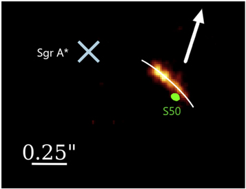
Figure 11. Possible evolution of the X7/S50 system. The sketch is based on the line map detection of X7 in 2018 at about 2.161 μm shown in Figure 5. The green-filled contour represents the K-band position of S50. The white curved line along X7 corresponds to the speculative scenario where the head of the system gets detached and attracted by Sgr A* (light-blue ×). The arrow indicates the direction of the proper motion of X7 and S50 as derived by Gillessen et al. (2009) and Mužić et al. (2010).
Download figure:
Standard image High-resolution imageAppendix C: X7, a Tidally Stretched Feature
As a rather speculative scenario, we shortly discuss the possibility that X7 is a tidally stretched gas and dust feature (as proposed by Randy Campbell, UCLA, at the GCWS 2019 proceedings, in preparation). Isolating the observation of X7/S50 in 2018 could indeed lead to the assumption that the source is a tidally stretched gas and dust feature (see Figure 11). Even though this scenario promises a wide range of useful scientific implications, observations of comparable objects have shown that a tidally stretched object is rather unlikely (Gillessen et al. 2012; Eckart et al. 2013; Valencia-S. et al. 2015). Considering Figure 4 (left side), we do find an increasing distance of the head from S50. However, the overall trend of the X7/S50 system seems to be not affected by Sgr A* (Figure 4, right side). Even with the observed and detected asymmetry regarding the stellar position with respect to its gaseous and dusty shell X7, the system is following the proper motion as found by Mužić et al. (2010). As pointed out several times, a long-time survey of the evolution of X7/S50 is required.
Appendix D: COMIC/ADONIS+RASOIR Data of 1999
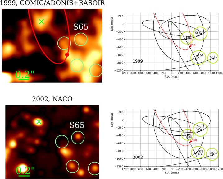
In Figure 12, we present the results of the long-time survey of X7 in the L'-band with COMIC/ADONIS+RASOIR (1999) in combination with the NACO data (2002, 2003–2018 are shown in Figure 2). For the image presented in Figure 12, which is observed with COMIC/ADONIS+RASOIR, we use a high-pass filter to highlight the features of the S-cluster. In both images, we clearly detect the structure of the S-cluster (Figure 12). Even though the resulting COMIC/ADONIS+RASOIR image of 1999 suffers from a decreased magnitude sensitivity, we are still able to identify several (isolated) sources, including the spherical shaped bow shock source X7 at the position of S50. As indicated by the orbital plots presented on the right-hand side of Figure 12, we identify the nearby S-cluster stars S33, S71/S72, S65, and S87 and mark them accordingly. Moreover, we include the K-band-based orbit of S50 (red dot) in the presented COMIC/ADONIS+RASOIR data of 1999 (red ellipse).
Figure 12. GC in the L'-band observed with COMIC/ADONIS+RASOIR and NACO in 1999 and 2002, respectively. The green × marks the approximate position of Sgr A*. In 1999 and 2002, the position of S2 and Sgr A* are confused because of their close proximity to each other. Some re-identified S-stars are marked with a light green circle. In 1999, the orbital spatial position of the S-cluster stars S71 and S72 coincide, which results in the bright spot marked with a light green circle. The right-hand side shows orbits of the S-stars S33 (marked), S50, S71/S72 (marked), and S87 (marked). The position of S65 can be used for orientation in these plots (see Figure 2 for a comparison). The orbit of S50 is highlighted in red. The empty circle of S33 in 2002 corresponds to the position of the star in the high-pass filtered image.
Download figure:
Standard image High-resolution image
Appendix E: Data
Here, we list the NACO and SINFONI data. Parts of these data were analyzed in various publications, e.g., Mužić et al. (2010), Witzel et al. (2012), Eckart et al. (2012), Zajaček et al. (2014), Valencia-S. et al. (2015), Shahzamanian et al. (2016), Parsa et al. (2017), and Peißker et al. (2019, 2020a, 2020b, 2020c, 2020d). These publications underline the robustness of the data use. For the sake of completeness, it should be noted that Parsa et al. (2017) derived with with data used here the gravitational redshift of S2 caused by the SMBH. This was later independently confirmed by the Gravity Collaboration et al. (2018) and indicates the quality of the data reduction process applied to the data.
Footnotes
- 7
COME-ON-PLUS Infrared Camera/Adaptive Optics Near Infrared System + Renouveau de l'Analyseur de Surface d'Onde InfraRouge
- 8
Since the nature of this source is better represented by the name DSO, we will use this throughout the manuscript.
- 9
Nasmyth Adaptive Optics System (NAOS) & Near-Infrared Imager and Spectrograph (CONICA)=NACO.
- 10
Gravity Collaboration et al. (2020) state 3 mas compared to 27 mas of the L'-band setting of NACO.
- 11
We advise the interested reader to compare the Brγ emission of 2008 and 2018 presented in Figure 5.
- 12
Discussed by Randy Campbell et al., UCLA, at GCWS 2019 (proceedings in preparation).
- 13
Transition v = 1–0 Q(1).
- 14
Transition v = 1–0 Q(3).
- 15
Transition 2p1 P0−2s1 S.