


Abstract
Metis, the space coronagraph on board the Solar Orbiter, offers us new capabilities for studying eruptive prominences and coronal mass ejections (CMEs). Its two spectral channels, hydrogen Lα and visible light (VL), will provide for the first time coaligned and cotemporal images to study dynamics and plasma properties of CMEs. Moreover, with the VL channel (580–640 nm) we find an exciting possibility to detect the helium D3 line (587.73 nm) and its linear polarization. The aim of this study is to predict the diagnostic potential of this line regarding the CME thermal and magnetic structure. For a grid of models we first compute the intensity of the D3 line together with VL continuum intensity due to Thomson scattering on core electrons. We show that the Metis VL channel will detect a mixture of both, with predominance of the helium emission at intermediate temperatures between 30 and 50,000 K. Then we use the code HAZEL to compute the degree of linear polarization detectable in the VL channel. This is a mixture of D3 scattering polarization and continuum polarization. The former one is lowered in the presence of a magnetic field and the polarization axis is rotated (Hanle effect). Metis has the capability of measuring Q/I and U/I polarization degrees and we show their dependence on temperature and magnetic field. At T = 30,000 K we find a significant lowering of Q/I which is due to strongly enhanced D3 line emission, while depolarization at 10 G amounts roughly to 10%.
Export citation and abstract BibTeX RIS
1. Introduction
Magnetic-field measurements in cool coronal structures like prominences, coronal rain, or coronal mass ejections (CMEs) represent a challenging problem. In the case of quiescent prominences, several attempts were made to determine the supporting magnetic fields using the spectro-polarimetry—for a review, see López Ariste (2015). Prominences are low-density media and thus the scattering of the incident solar radiation determines their emissivity. Their illumination by the solar disk is largely anisotropic, which leads to a linear polarization of the scattered radiation. The presence of a magnetic field, which is rather weak in prominences, then causes a lowering of the polarization degree and rotation of the polarization plane (the Hanle effect; see Landi Degl'Innocenti & Landolfi 2004). Typical range of the magnetic-field strength in quiescent prominences is around 10 G, but fields as high as tens of G have also been reported (López Ariste 2015). Recently, a much stronger field was detected in post-flare loops, previously referred to as loop prominences and nowadays identified as coronal rain. However, in the case of flare loops with a field strength of a few hundreds of Gauss, the polarization is due to the Zeeman effect and the weak-field approximation was used to determine the field strength (Kuridze et al. 2019). Another class of relatively cool coronal structures is represented by cores of CME, where the kinetic temperatures are on the order of 104–105 K or more (see, e.g., Heinzel et al. 2016 and Jejčič et al. 2018). In these structures, however, the magnetic field was never measured. This is related to the fact that CMEs are mostly observed from space, using coronagraphs in visible light (e.g., LASCO on board SOHO and COR1 and COR2 on board STEREO missions) or with the UV spectrograph like UVCS on board SOHO. Nevertheless, there are no spectropolarimeters attached to space coronagraphs capable of measuring the linear polarization in spectral lines emitted by prominence-like structures including CME cores. A giant coronagraph ASPIICS on board the ESA's Proba-3 formation-flight mission (Lamy et al. 2017) will detect the helium D3 line at 587.73 nm (vacuum wavelength), but only the integrated intensity and no polarization. D3 line polarization in prominence-like structures was studied in many cases, both theoretically as well as observationally (see López Ariste 2015) and, therefore, some attempts were made to include D3 polarization measurements in the concept of ASPIICS. But due to different reasons the final setup will provide polarization detection only in the broadband visible channel, which is important for determinations of the electron density.
With the launch of the ESA-NASA Solar Orbiter mission, we find an exciting opportunity to detect the D3 line polarization in eruptive prominences and CMEs, using the Metis coronagraph (for a description of Metis, see Antonucci et al. 2019). This is because the visible-light (VL) continuum channel of Metis in the range between 580 and 640 nm contains the D3 line at its wavelength edge, which is still detectable, and this channel will provide the polarization measurements. Note that Metis has additional imaging capability in the hydrogen Lyman α line, which will provide important diagnostics of the CMEs and coronal plasmas. The situation with the Metis VL channel is similar to that of SOHO/LASCO-C2, where the orange VL channel also contains the helium D3 line. Quite recently, Floyd & Lamy (2019) analyzed several CMEs detected in the orange channel of LASCO-C2, and they discussed apparent signatures of the D3 polarization. On the other hand, Dolei et al. (2014) were able to extract the Hα line polarization in a CME combining STEREO-COR1 and LASCO-C2 observations and they suggested that this could be used to determine the magnetic field in CMEs.
Our idea is to use the Metis VL channel to detect the D3 polarization in CMEs and possibly to measure their magnetic fields. The main difficulty is that the expected line polarization is mixed with the linear continuum polarization, which is due to Thomson scattering on CME electrons. In this paper we theoretically estimate the amount of D3 line polarization under typical CME conditions and compare it with the respective continuum component. Then we discuss possibility of the magnetic-field determination based on Metis observations.
2. Models of Eruptive Prominences and CMEs
For the purpose of this exploratory work we use the prominence-CME models as described by Jejčič et al. (2018) who studied the capabilities of the narrowband D3 filter for ASPIICS. Since the temperatures in those models range from 8000 K up to 105 K, the models we select here can represent cool erupting prominence plasma as well as hot cores of CMEs (Heinzel et al. 2016). The electron densities ne are first computed with the hydrogen code and then used to synthesize the helium lines as in Labrosse & Gouttebroze (2001, 2004). Note that we neglect here the effect of potentially large CME velocities on the electron density, an aspect to be considered in future modeling. Such velocities, however, do not affect the formation of the D3 line because the prominence is illuminated by continuum radiation, i.e., no Doppler brightening effect takes place. D3 line-center optical thickness τ0 is the input parameter for our polarized radiative-transfer modeling. We need to know the relation between τ0 and ne in order to consistently evaluate the D3 and VL emissions that enter the Metis filter passband. From a grid of 90 models computed in Jejčič et al. (2018) we selected 20 representative ones as shown in Table 1. We choose two heights above the solar surface, and namely 800 Mm with geometrical dilution factor W = 0.058 and 1600 Mm with W = 0.024, which correspond to 2.15 and 3.30 solar radii measured from the disk center, respectively, in the range covered by Metis at its closest approach to the Sun. The dilution factor W substantially decreases with height, which lowers the amount of exciting radiation but simultaneously increases its anisotropy. For the effective geometrical thickness D we choose 5 Mm, which, together with a low filling factor (Susino et al. 2018), represents plausible sizes of CME cores. The selected gas pressures produce hydrogen ionization comparable to that in situations of eruptive prominences and hot CMEs. Similarly to Jejčič et al. (2018), we increase the microturbulent velocity with increasing temperature (see the case or a CME flux rope in Jejčič et al. 2017).
Table 1. Grid of Models Used for Synthesis of Polarized Radiation in D3 Line and VL
| Model | h | T | p | D | vt | ne | E(D3) | τ0(D3) | E(VL) |
|---|---|---|---|---|---|---|---|---|---|
| (km) | (K) | (dyn  ) ) |
(km) | (km s−1) | (cm−3) | (cgs) | (cgs) | ||
| 1 | 800,000 | 8000 | 0.05 | 5000 | 5 | 3.83+9 | 44.2 | 8.4–4 | 90.3 |
| 2 | 800,000 | 15,000 | 0.05 | 5000 | 5 | 1.15+10 | 34.9 | 5.2–4 | 271.0 |
| 3 | 800,000 | 30,000 | 0.05 | 5000 | 15 | 6.29+9 | 885.0 | 6.7–3 | 148.2 |
| 4 | 800,000 | 50,000 | 0.05 | 5000 | 15 | 3.78+9 | 176.9 | 1.2–3 | 89.1 |
| 5 | 800,000 | 100,000 | 0.05 | 5000 | 20 | 1.89+9 | 2.8 | 1.6–5 | 44.5 |
| 6 | 800,000 | 8000 | 0.1 | 5000 | 5 | 8.35+9 | 35.8 | 6.8-4 | 196.8 |
| 7 | 800,000 | 15,000 | 0.1 | 5000 | 5 | 2.34+10 | 66.1 | 9.5-4 | 551.5 |
| 8 | 800,000 | 30,000 | 0.1 | 5000 | 15 | 1.26+10 | 2244.4 | 1.6–2 | 297.0 |
| 9 | 800,000 | 50,000 | 0.1 | 5000 | 15 | 7.56+9 | 439.8 | 2.7–3 | 178.2 |
| 10 | 800,000 | 100,000 | 0.1 | 5000 | 20 | 3.78+9 | 6.9 | 3.6–5 | 89.1 |
| 11 | 1,600,000 | 8000 | 0.05 | 5000 | 5 | 1.75+9 | 7.5 | 3.3–4 | 16.5 |
| 12 | 1,600,000 | 15,000 | 0.05 | 5000 | 5 | 1.13+10 | 6.9 | 2.0–4 | 106.5 |
| 13 | 1,600,000 | 30,000 | 0.05 | 5000 | 15 | 6.29+9 | 290.4 | 3.7–3 | 59.3 |
| 14 | 1,600,000 | 50,000 | 0.05 | 5000 | 15 | 3.78+9 | 57.9 | 6.2-4 | 35.6 |
| 15 | 1,600,000 | 100,000 | 0.05 | 5000 | 20 | 1.89+9 | 0.9 | 8.2-6 | 17.8 |
| 16 | 1,600,000 | 8000 | 0.1 | 5000 | 5 | 4.07+9 | 6.1 | 2.6–4 | 38.4 |
| 17 | 1,600,000 | 15,000 | 0.1 | 5000 | 5 | 2.31+10 | 20.3 | 5.3-4 | 217.7 |
| 18 | 1,600,000 | 30,000 | 0.1 | 5000 | 15 | 1.26+10 | 850.9 | 8.7-3 | 118.8 |
| 19 | 1,600,000 | 50,000 | 0.1 | 5000 | 15 | 7.56+9 | 170.0 | 1.4–3 | 71.3 |
| 20 | 1,600,000 | 100,000 | 0.1 | 5000 | 20 | 3.78+9 | 2.6 | 1.8–5 | 35.6 |
Download table as: ASCIITypeset image
3. Helium D3 Line Formation in Prominences and CMEs
Formation of the helium D3 line under non-LTE conditions (i.e., departures from the Local Thermodynamic Equilibrium) is a complex multilevel radiative-transfer problem. For the case of solar prominences, it was treated in detail by Heasley et al. (1974) and later on by Labrosse & Gouttebroze (2001, 2004; see also reviews by Labrosse et al. 2010 and Labrosse 2015). The latter authors used a multilevel He i model atom depicted in Figure 1, and solving the multi-ion statistical equilibrium equations, they obtained the ionization structure, level populations, and optical properties of the helium. Here we will focus only on the formation of the D3 line, which can be approximately separated into two problems: the excitation of level 9 from which the optically thin D3 emission arises, and the population of the lower level 4, which determines the optical thickness τ0 of the D3 line (see Table 1). While the first aspect can be treated as a two-level atom problem, the second one is a complex multilevel and multi-ion non-LTE problem. Optical thickness  and integrated intensity of D3 result from the helium multilevel modeling as described in Labrosse & Gouttebroze (2001); note that the helium non-LTE code uses as input the electron density previously computed with the hydrogen code. These quantities are shown in Table 1, together with the visible-light (VL) intensity integrated over the Metis VL passband 580–640 nm. VL emission is due to Thomson scattering on prominence or CME electrons and was computed using the limb-darkened incident continuum radiation from the solar disk (e.g., Cox 2000). We can see from Table 1 that even using this wide-band Metis filter, the D3 line intensity is not negligible in comparison to VL intensity and namely for higher temperatures around 30–50,000 K the D3 intensity dominates the VL one. This means that we may expect a nonnegligible contribution of D3 to total polarization signal from the Metis filter. This is also consistent with the conclusions of Floyd & Lamy (2019) who found CME signatures of the D3 emission within an even wider (100 nm) broadband orange filter of the LASCO-C2 coronagraph. The first question that arises is how the upper level 9 of the D3 transition is excited. In Jejčič et al. (2017) the authors suggest that much brighter D3 at T = 30,000 K can be due to stronger collisional excitations at higher temperatures. This of course would produce an unpolarized emission, i.e., the scattering term will be negligible compared to the collisional one in the line source function. We know that collisions, both inelastic as well as elastic, are negligible at typical prominence temperatures below say 10,000 K, but how will they be at the much higher temperatures found in CME cores? In order to answer this critical question, we made two calculations. First, we quantitatively compared the collisional excitation rates to upward radiative ones (i.e., those leading to scattering). Their ratio is

where B49 is the Einstein coefficient for absorption, I0 is the disk-center continuum intensity at the D3 wavelength, and W is the geometrical dilution factor (in this estimate we neglect the continuum limb darkening). C49 is the collisional rate depending on temperature. We found that for all models considered here this ratio is quite small, and the radiative rates are several orders of magnitude larger than the collisional ones, even at high temperatures. This is good news since the line source function in this two-level model is dominated by scattering. We also found negligible collisional rates for transition between levels 2 and 4, which means that level 4 is populated by radiative excitation and thus is polarized (see the next section).

Figure 1. Atomic level and transition diagram for He i atom. The wavelengths of line transitions are indicated, and the dashed line represents the ionization continuum from the ground state. This line also schematically divides the singlet and triplet states of He i. Here the D3 line is due to the transition between levels 4 and 9.
Download figure:
Standard image High-resolution imageThe other independent calculation shows that all D3 line intensities from Table 1 result from an almost identical line source function that is dominated by scattering. For the line integrated intensity we can simply write

where ΔλD is the line Doppler width and S is the line source function. Using E, ΔλD, and τ0 according to Table 1, we find that resulting source function S is almost identical for all models. This then means that it must be dominated by scattering at higher temperatures also.
However, there is still the question of why D3 brightness is so large at temperatures around 30,000 K and this is the other aspect of the D3 line formation problem. Looking at Equation (2) we see that, for a fixed S, E varies due to changes of ΔλD and τ0. However, the product ΔλD × τ0 is directly proportional to number density of He i atoms in level 4, i.e., the level 4 population. Since level 4 is mainly populated by radiative excitations from level 2, i.e., the scattering in the 1083 nm line (collisional excitation is again negligible at low densities), the temperature dependence of τ0(D3) must follow that of the second level population. It is generally known that this particular triplet state is populated by recombinations (radiative and di-electronic) from the He ii ion. Therefore, it must depend on the ionization rate from He i to He ii. If this population is dependent on temperature, the collisional ionization of He i from its ground state must dominate over the radiative one. We thus computed these two rates. The radiative (photoionization) rate was estimated using the incident EUV ionizing radiation below 50.4 nm and the collisional ionization rates were computed according to Mihalas & Stone (1968). Very interestingly, around T = 30,000 K, the collisional ionization is already dominant over the photoionization by almost one order of magnitude while at low temperatures it is quite negligible. Therefore, we may expect a significant temperature-dependent increase of He ii density and thus also of population of the triplet ground state 2 due to photorecombinations. However, for much higher temperatures reaching 105 K, τ0(D3) will substantially decrease due to strong ionization of helium (see Table 1). In summary, we see that E(D3) is varying with temperature due to He i collisional ionization and subsequent photorecombinations, but the line source function is completely dominated by scattering. Note that a slight difference from such a source function at high temperatures is probably due to recombinations directly to level 4.
4. Visible-light and D3 Scattering Polarization
4.1. Visible-light Component
For the sake of simplicity, we consider a simple scattering geometry as shown in Figure 2. The plasma located in the plane of the sky at the height h above the solar surface is illuminated by an anisotropic radiation from the underlying solar photosphere. We assume the illumination is due to an unpolarized solar continuum radiation in the whole spectral interval of the VL filter. Due to the limb darkening effect, the incident intensity Iinc(λ, θ) at wavelength λ depends on the incident angle θ. In our calculations, we use interpolated data from Cox (2000) for Iinc(λ, θ).
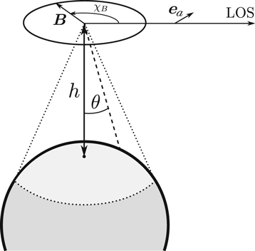
Figure 2. Scattering geometry considered in this paper. The plasma is located at the height h above the solar surface and scatters the incident disk radiation that arrives at the angle θ between the local vertical and the direction of illumination. The positive Stokes Q direction (i.e., the  vector) is parallel to the nearest solar limb. The magnetic field vector
  is perpendicular to the solar radius and deviates by an angle χB from the line of sight (LOS) that is chosen to be perpendicular to the local vertical direction.
Download figure:
Standard image High-resolution imageThe VL continuum emission is predominantly due to the Thomson scattering. In order to calculate the intensity and linear polarization of the scattered radiation at a given height and wavelength, two components of the radiation field tensor need to be considered, namely  that corresponds to the common mean radiation field intensity J, and
  that quantifies anisotropy of the incident field:


where μ = −cos θ (for more details, see Landi Degl'Innocenti & Landolfi 2004). In Figure 3, we show the height dependence of these quantities at the wavelength λ = 600 nm. Even though these quantities depend on wavelength, this dependence is rather weak in the interval of interest (580–640 nm). As is evident from the plot, the fractional anisotropy  rapidly increases with height, as does the fractional polarization of the emitted VL radiation (see below).

Figure 3. Mean intensity ( ) and fractional anisotropy (
 ) as a function of height above the solar surface at the wavelength
  .
.
Download figure:
Standard image High-resolution imageThe continuum optical thickness of the slab of free electrons is independent of wavelength and equal to  , where ne is the electron number density,
  is the Thomson scattering cross-section, and D is the geometrical thickness of the slab. In the models considered in this paper, we are always in the regime of very small optical thickness, τe ≪ 1. In that case, the scattered continuum intensity (Stokes parameter I) and linear polarization (Stokes parameter Q) in the geometrical configuration of Figure 2 are equal to the respective Stokes source functions SI and SQ multiplied by the optical thickness of the medium. The source functions of the Stokes parameters can be easily derived (e.g., Trujillo Bueno & Shchukina 2009) and the expressions for the emergent Stokes parameters read


We note that at heights above h ≈ 0.1R⊙, the second term in Equation (5) is not negligible (see Figure 3) and since  , the emitted intensity is lower than one would expect if anisotropy and polarization phenomena were neglected.
Integration of the above expressions over the Metis VL passband gives us the observable total emissivities of VL in intensity and linear polarization,


where ϕ(λ) is a normalized spectral sensitivity of the instrument. For the sake of simplicity, we consider ϕ(λ) = 1 in the range between 580 and 640 nm (see Antonucci et al. 2019).
The linear polarization of the VL is parallel to the nearest solar limb, i.e., the Stokes parameter U and  are equal to zero, and it is insensitive to the presence of magnetic field. In contrast to Thomson scattering, the linear polarization of the D3 line is sensitive to the magnetic fields via the Hanle and Zeeman effects. If the wavelength-integrated signal is contaminated by the photons emitted by the He i atoms, the EI, EQ, and EU can, in principle, provide information on the magnetic field vector in the slab.
4.2. Spectral Line Component
As shown by Bommier (1977), once the density of orthohelium is known from the non-LTE calculation, the atomic model sufficient for synthesis of the D3 line intensity and polarization consists of the terms 2, 4, 6, 8, and 9 in Figure 1 with a total of 11 fine-structure levels. In the low-density plasma of our interest, the depolarizing collisions can be neglected (Sahal-Brechot et al. 1977). Since the optical thickness of D3 (and presumably of the other considered lines) is smaller than one (see Table 1) and since the incident photospheric radiation is spectrally flat across the D3 line and, to a large extent across the other relevant lines of the model atom, the suitable picture of atomic levels is the multi-term approximation of Section 7.6 of Landi Degl'Innocenti & Landolfi (2004) and the discussion in Section 13.4 therein.
For the synthesis of the D3 line we use the code HAZEL (Asensio Ramos et al. 2008), which is applicable in the regime of our interest, namely in the limit of a constant-property slab. Given the height above the solar disk, magnetic field vector, and optical thickness of the slab obtained from the multi-ion non-LTE solution, we can calculate the line Stokes profiles and normalize the spectrum to the integrated absolute emissivity obtained from the unpolarized non-LTE solution (see Table 1). HAZEL uses the same five-term model atom as discussed above and takes properly into account the limb darkening effects in all the spectral lines.
At first, we consider the case of nonmagnetic plasma (B = 0 G) and we calculate the dependence of the total (VL and D3) integrated intensity and fractional polarization for different models. The results can be found in Figure 4. We see a significant depolarization effect due to the D3 line that is most apparent at intermediate temperatures around 30,000 K. This is closely related to the fact that at these temperatures the D3 line is extremely bright, hence both the intensity and fractional polarization signal are dominated by the line instead of the VL (see Table 1). Since fractional polarization of the line is always smaller than polarization of the VL, the presence of the line always leads to depolarization of the total signal (i.e., lowering of the fractional polarization). We note that fractional polarization of the line,  is practically insensitive to the model in the range of parameters of Table 1 and it only depends on the height above the solar surface and on the local magnetic field vector. In the following section, we discuss the magnetic sensitivity of the total VL+D3 signal.

Figure 4. Left panel: integrated intensity EI(D3+VL). Right panel: integrated linear-polarization degree EQ(D3+VL)/EI(D3+VL) signal. The signals for two different heights above the solar surface and two different plasma pressures are plotted as functions of kinetic temperature. The horizontal dotted lines in the right panel show the fractional polarization of the VL, neglecting the D3 contribution, at the heights h = 0.8 × 10⁶ km (black line) and 1.6 × 10⁶ km (blue line).
Download figure:
Standard image High-resolution image5. Magnetic Field and the Hanle Effect
5.1. Flux-rope Magnetic Field in CMEs
Measurements of magnetic fields in solar prominences are very difficult (see, e.g., the review by López Ariste 2015) and usually require long integration times in order to detect weak polarization signals. To our knowledge, the magnetic field inside erupting prominences has never been measured during the eruption in the expansion phase across the intermediate corona (what will be observed by Metis). However, in a recent paper by Fan et al. (2018) the authors simulate the appearance of an erupting prominence with the COSMO coronagraph, with the aim of demonstrating the feasibility of magnetic field determination from circular polarization measurements of the Fe xiii line undergoing the Zeeman effect. This paper provides the BLOS (i.e., the LOS averaged magnetic field) inside an erupting prominence at different times during the eruption. From their Figures 3, 11, and 15, in the early eruption phase (below 1.4 solar radii from the disk center) one can assume a maximum of 5–10 G at the center of the flux rope. For larger altitudes, we have to make some empirical considerations. Assuming that the flux rope is expanding self-similarly, and using a well known empirical relationship between the radial speed vrad and the expansion speed vexp of a CME,  (Dal Lago et al. 2003), one can assume that
  and the same relationship holds between the altitude of the CME and the radius of the flux rope. This means that the cross-sectional area AFR of the flux rope is going with the CME altitude hCME like

Now, if we assume the magnetic flux conservation during the expansion, we can write that  . Therefore, as an order of magnitude estimate, if for instance B(0) = 10 G when hCME = 1.2RSun (Figure 11 from Fan et al. 2018) then for a CME at 3
  the magnetic field is
  G. One can use the same empirical relationship to rescale the field at higher/lower altitudes if required.
5.2. Magnetic Sensitivity and the Simulated Hanle Diagrams
While the VL signal is insensitive to the magnetic field, the linear polarization of D3 can be modified by the magnetic field due to the Hanle and Zeeman signals. In Figure 5 we show the dependence of the total fractional linear polarization signals of the VL+D3 on the magnetic field strength. Even a very weak magnetic field (B < 1 G) causes partial relaxation of the quantum coherence in the  and
and  levels leading to the lower-level Hanle effect, hence to a sensitivity of the polarization signal to sub-G fields (Bommier 1980). At fields on the order of a few G, the signal is highly sensitive to the upper-term Hanle effect in
  . Above ≈6 G, the J-level crossings start to occur and the upper term enters the so-called incomplete Paschen–Back effect (see, e.g., Sahal-Brechot 1981). These effects are most obvious in the central panels of Figure 5, where the D3 line dominates the total signal while in the cooler or hotter plasmas the depolarization and rotation of the polarization vector are less obvious.

Figure 5. Total (i.e., VL and D3) fractional polarization signals EQ/EI (left panels) and EU/EI (right panels) for different models as a function of magnetic field intensity. From top to bottom, the panels show models with temperatures of 8000, 30,000, and 100,000 K. The magnetic field is oriented along the LOS (χB = 0°).
Download figure:
Standard image High-resolution imageThe Hanle diagrams shown in Figure 6 further demonstrate the sensitivity of the linear polarization signal to different magnetic field strengths and orientations. It follows that the main impact of the D3 line is a lowering of the fractional polarization EQ/EI due to relatively high D3 intensity at temperatures around 30–50,000 K. However, for certain combinations of magnetic field strength and orientation, the Hanle effect can leave measurable signatures in the linear polarization signal. For instance, at B = 3 G and χB = 0°, the polarization vector can be rotated by about 10° with respect to the nearest solar limb, thus providing measurable positive evidence for the presence of magnetic field. In other cases, depolarization of the Stokes Q parameter still provides a valuable constraint on the thermal conditions of the CME plasma.

Figure 6. Polarization (or Hanle) diagrams of the VL+D3 signal for three different plasma temperatures, height h = 1.6 × 10⁶ km, and  . The solid lines correspond to the magnetic field of a fixed strength and changing azimuth χB (indicated in the central panel). The dotted lines show the signals for fixed magnetic field azimuth and varying strength. The signal of VL, i.e., neglecting the D3 contribution, is shown by the blue dot on the top of the panels.
Download figure:
Standard image High-resolution image
6. Discussion and Conclusions
In order to detect signatures of the D3 line emission in the integrated signal from the VL filter of Metis, we must estimate the relative intensities of the line and VL continuum, which are due to Thomson scattering on free electrons in the CME core. The core is usually well recognized as a bright flux rope or a patchy prominence-like structure, see, e.g., Heinzel et al. (2016) or Floyd & Lamy (2019; their Figure 1) so that we can neglect other VL contributions due to a CME halo (quiet-corona emission is normally subtracted from images). Our theoretical estimates for a range of plausible CME-core models are given in Table 1, where we can see that the D3 contribution is nonnegligible and in the temperature range between 30,000 and 50,000 K it significantly dominates over the VL one (we discuss this behavior in Section 3). We know that such temperatures are present inside CME cores, see, e.g., Jejčič et al. (2017). At 30,000 K, the D3 line is a factor of 5–7 brighter compared to VL. At low temperatures VL signal dominates and at 105 K the line contribution is less that 10%.
Normally one cannot infer a dominance of the line emission over the VL continuum just from the fact that the CME core is structured like a cool prominence (see Figure 1 in Floyd & Lamy 2019 and the caption). This is because the CME-core electron densities will produce a similar pattern in VL due to Thomson scattering. However, we can disentangle between these two contributions using linear polarization measurements. Looking at Figure 4 (right panel), we see that for temperatures between say 20,000 and 80,000 K the polarization degree EQ/EI is significantly lower compared to a constant 80%–90% polarization, which is only due to Thomson scattering. This corresponds to an intensity enhancement (peak) in the left panel of Figure 4, which is due to D3 emission. Our models can thus, at least qualitatively, explain the behavior of LASCO-C2 observations analyzed by Floyd & Lamy (2019). LASCO-C2 orange filter is even wider (540–640 nm) than the Metis VL filter, and also contains the D3 line (in its central part). At least in two cases analyzed by these authors, the detected polarization is surprisingly low compared to expected high-degree polarization due to Thomson scattering alone. The authors thus conclude that this might be due to the presence of the D3 line and they consider possible depolarization due to the Hanle effect. But since we know the brightness of the D3 line in our models, we see that the line is sometimes very bright and therefore total EQ over total EI is low even in a nonmagnetic case. It is interesting to note that a low polarization was also detected in a CME by Mierla et al. (2011) using the wide-band filter of SECCHI/COR1 coronagraph, which contains the hydrogen Hα line in its center. Note that this line is typically much brighter in cool prominence structures as compared to D3.
At this point we should mention that both Metis as well as LASCO-C2 filters contain a Na i doublet redward of the D3 line at 589.16 and 589.76 nm (the rest wavelength). These lines are also in emission in prominence-like structures and thus may contaminate the total VL signal. However, as thoroughly discussed in Jejčič et al. (2018), their typical brightness is much lower compared to the D3 line and thus we neglect them in our present analysis.
Based on our estimation of the magnetic-field strength in CMEs, we studied the Hanle effect on the D3 line. Concerning the orientation of the magnetic-field vector in a CME core, we can at least see from numerous observations that the expanding flux rope top is more or less parallel to the solar limb and this is very favorable for the field detection via the Hanle effect in the D3 line. Our results are presented and briefly discussed in Section 5. We show that under some conditions it will be possible to diagnose CME magnetic field using the VL channel of Metis. At low temperatures (our models with 8000 K) and for B around 10 G, the Hanle depolarization is only by about 2% (similar to quiescent prominences), at 105 K it is even lower. But for intermediate temperatures the depolarization amounts to 10% or more—see polarization diagrams in Figure 6. At 30,000 K we see a significant lowering of polarization degree due to D3 brightness, plus about 10% lowering due to the 10 G magnetic field. The polarization capabilities of Metis are described in Antonucci et al. (2019) and Fineschi et al. (2020) and in a following paper we plan to perform a more detailed analysis of the Metis VL-channel response to magnetic-field and thermal structure of CMEs. In parallel we are studying the diagnostics potential of the Metis Lyman α channel, which can provide independent information on CME thermal structure. Finally, D3 line intensity (i.e., Stokes I) and broadband VL polarization will be detected by the ASPIICS coronagraph on board ESA's Proba-3 formation-flight mission and thus synergy with Metis will be of great interest.
The Solar Orbiter is the ESA mission toward the Sun launched by NASA on 2020 February 10. Metis is its payload coronagraph developed by the Italian–German–Czech consortium, under the leadership of Italian ASI. The authors acknowledge support from grant Nos. 19-17102S and 19-20632S of the Czech Funding Agency and from RVO:67985815 project of the Astronomical Institute of the Czech Academy of Sciences. The Czech contribution to Metis was funded by ESA-PRODEX. S.J. acknowledges support from the Slovenian Research Agency No. P1-0188. N.L. acknowledges support from the Science and Technology Facilities Council (STFC) Consolidated grant No. ST/ P000533/1.
Facility: Solar Orbiter—Metis. -