


Abstract
The goal of this paper is to derive the physical conditions of the prominence observed on 2017 March 30. To do so, we use a unique set of data in Mg ii lines obtained with the space-borne Interface Region Imaging Spectrograph (IRIS) and in Hα line with the ground-based Multi-Channel Subtractive Double Pass spectrograph operating at the Meudon solar tower. Here, we analyze the prominence spectra of Mg ii h and k lines, and the Hα line in the part of the prominence which is visible in both sets of lines. We compute a grid of 1D NLTE (i.e., departures from the local thermodynamical equilibrium) models providing synthetic spectra of Mg ii k and h, and Hα lines in a large space of model input parameters (temperature, density, pressure, and microturbulent velocity). We compare Mg ii and Hα line profiles observed in 75 positions of the prominence with the synthetic profiles from the grid of models. These models allow us to compute the relationships between the integrated intensities and between the optical thickness in Hα and Mg ii k lines. The optical thickness τHα is between 0.05 and 2, and  is between 3 and 200. We show that the relationship of the observed integrated intensities agrees well with the synthetic integrated intensities for models with a higher microturbulence (16 km s−1) and T around 8000 K, ne = 1.5 × 1010 cm−3, p = 0.05 dyne. In this case, large microturbulence values could be a way to take into account the large mixed velocities existing in the observed prominence.
Export citation and abstract BibTeX RIS
1. Introduction
Solar prominences are an important part of the solar corona, as they may often trigger solar eruptions and are generally a part of the coronal mass ejections (CMEs); see, e.g., Schmieder et al. (2015), Ruan et al. (2014, 2015), and Heinzel et al. (2016). The prominence plasma temperature is relatively low compared with the temperature of its coronal environment by roughly two orders of magnitude (Labrosse et al. 2010). The prominence magnetic field, which supports the cool and dense prominence plasma against gravity (Mackay et al. 2010), also plays an insulation role because the thermal conduction is very weak across the magnetic field (Démoulin et al. 1987). As the prominences expand and leave the solar surface, they contribute to mass loading of CMEs (Heinzel et al. 2016; Jenkins et al. 2019), representing the core of a CME. Knowing their physical parameters, e.g., the kinetic temperature, gas pressure, electron density, and microturbulence would constrain the extensive magnetohydrodynamic numerical simulations of CMEs containing a cool flux rope inside (Pagano et al. 2014). The role of the prominence mass in CME is detailed in different articles in Schmieder et al. (2014a).
Owing to the particular prominence plasma conditions of high density and low temperature, the interpretation of the prominence spectral observations requires multi-level NLTE (i.e., departures from the local thermodynamical equilibrium) radiative transfer models. Such prominence radiative transfer models in one-dimensional (1D) or two-dimensional (2D) have been developed by e.g., Gouttebroze et al. (1993), Paletou et al. (1993), Heinzel & Anzer (2001), Gunár et al. (2007, 2008, 2014), Heinzel (2015), Labrosse (2015), and Levens & Labrosse (2019). Analysis of spectroscopic data using the NLTE models allows for the determination of several plasma parameters such as kinetic temperature, density, gas pressure, bulk velocities, and ionization state (see, e.g., Heinzel et al. 2001; Labrosse et al. 2010; Gunár et al. 2012; Park et al. 2013; Heinzel 2015; Labrosse 2015).
Simultaneous imaging and spectral capabilities of the Interface Region Imaging Spectrograph (IRIS; De Pontieu et al. 2014) have been demonstrated to be a very powerful tool for the investigation of the dynamics and the physical conditions of the solar prominences by, e.g., Schmieder et al. (2014b), Liu et al. (2015), Levens et al. (2016a, 2016b), or Ruan et al. (2018, hereafter Paper I). For prominences, a set of four spectral lines (C ii, Mg ii h and k, Si iv) is commonly observed by IRIS. Complex Mg ii profiles with several asymmetric peaks that occur in the IRIS observations have been explained by the presence of prominence fine structures moving with different velocities located along the line of sight (LOS) (Heinzel et al. 2015). In such a case, the decrease of the intensity of individual spectral components with the distance from line center is consistent with the Doppler dimming effect (Heinzel et al. 2015). C ii line profiles can be used to confirm the existence of such multiple, dynamic structures along the LOS (Paper I).
The double-peaked Mg ii profiles can be caused also by a high optical thickness of the prominence plasma in these lines, as shown by Levens et al. (2016a) and Jejčič et al. (2018). Moreover, in some prominences, the Mg ii profiles can exhibit also nonreversed shapes (see, e.g., Paper I).
Using the 1D NLTE radiative transfer model, Heinzel et al. (2014) showed that the nonreversed profiles can be reproduced by models with low gas pressure (p = 0.01 dyne cm−2) and the reversed profiles by models with higher gas pressures (p = 0.5 dyne cm−2). Jejčič et al. (2018) statistically studied the reversal of the observed and synthetic Mg ii h and k line profiles. Those authors did not find a complete agreement between the results of 1D isothermal and isobaric models and the IRIS observations. Their study focused on a limited part of the observed prominence and considered only Mg ii spectra. However, for another prominence observed in both Hα and in Mg ii lines, Heinzel et al. (2015) showed that when the Prominence-Corona Transition Region (PCTR) is taken into account, the gas pressure corresponding to nonreversed profiles could reach a value equal to p = 0.07 dyn cm−2, which is significantly higher than the value obtained without PCTR (Heinzel et al. 2014). Low-pressure values lead to low optical thickness in the Hα line, and because Mg ii lines has an optical thickness 100 times larger than Hα, a prominence can be visible in Mg ii lines and transparent in Hα (Heinzel et al. 2015).
In the present paper, we focus on the analysis of the physical conditions of a quiescent prominence observed on March 30, 2017 with IRIS in Mg ii , C ii and Si iv lines and also in the Hα line with the Multi-channel Subtractive Double Pass (MSDP) spectrograph operating at the Meudon solar tower. This set of data is relatively unique. In Section 2 we briefly summarize the observations. In Section 3 we present spectroscopic results that combine the observations in Hα and in Mg ii. We compute the ratio between integrated intensities of Mg ii k and h lines for prominence compared with the solar disk and for parts of the prominence visible in Hα and not visible in Hα. The integrated intensity of Mg ii k and h allows us to determine the difference of optical thickness of Mg ii in both situations, as suggested by models of Jejčič et al. (2018). After a careful coalignment of pixels in Mg ii spectra and pixels in Hα spectra, we identify a list of 75 overlapping pixels and derive the ratio between the integrated intensities of Mg ii and Hα in these pixels.
In Section 4 we present a grid of 1D NLTE models with several varying input parameters (e.g., temperature, pressure, geometrical thickness, and microturbulent velocity). The large microturbulence needed for the fitting is a way to interpret the large broadening (FWHM) of Hα line in terms of mixed bulk velocities present in multiple prominence fine structures intersected by a LOS.
2. Observations of the 2017 March 30 Prominence
2.1. Instruments
The prominence was the target of an international campaign on 2017 March 30 with IRIS and ground-based instruments, e.g., the MSDP spectrograph (Figure 1). It was located on the northwest limb and extended along 120 arcsec with a maximum height of 30,000 km. IRIS provided high-resolution imaging and spectroscopic observations of this prominence. Details of these observations have been presented in Paper I.
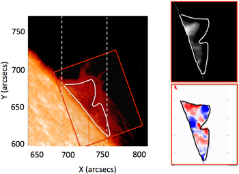
Figure 1. Left panel: IRIS slit-jaw images (SJIs) in 2796 Å on 2017 March 30 at 07:06:28 UT overlaid with white contours of the Hα prominence. The red box with a size of 80'' × 120'' indicates the field of view from the right panels. Right panels: Hα prominence intensity (top) and Doppler shift observed with MSDP (bottom) on 2017 March 30 at 07:28 UT. The contour corresponds to the intensity value higher than a defined threshold. Blue/red indicates blueshift/redshift limited to ±7 km s−1. Two white dashed vertical lines in the IRIS SJI image show the limits of the field of view of the IRIS rasters. The red vertical line on the disk indicates the IRIS slit position at the time of SJI.
Download figure:
Standard image High-resolution imageIn the present paper, we use the coarse raster data obtained in the doublet of Mg ii h (2803.5 Å) and k (2796.4 Å) lines using 32 positions of the slit covering an area of 64'' × 120'' with a step of 2'' between two spectra and a pixel size of 0 33. Between 07:06 UT and 08:46 UT, six raster scans were recorded with a cadence of 15 minutes per raster, resulting in a total of 192 spectra (6 × 32).
Calibrated level-2 data are used in this study. Dark current subtraction, flat-field correction, and geometrical correction have been taken into account in the level-2 data (De Pontieu et al. 2014). Slit-jaw images (SJIs) in the broadband filter 2796 Å with its large field of view (167'' × 175'') have been used for the coalignment. One example of a SJI is presented in Figure 1 left panel.
The MSDP operating on the solar tower in Meudon observed the same prominence in the Hα line. The entrance field stop of the spectrograph covers an elementary field of view of 60'' × 450'' with a pixel size of 05. Using the MSDP technique (Mein 1977; Mein & Mein 1991; Mein 1991), the Hα image of the field of view is divided by wavelengths into nine channels covering the same channel field of view. The nine channels are recorded simultaneously on a CCD Princeton camera. In Figure 2 an example of observation of the disk with nine channels and the reconstruction of the profile using a point in each channel are shown. Each image is obtained in a different wavelength interval. The wavelength separation between the center wavelength of one channel image to the next is 0.3 Å. By interpolating using cubic spline functions between the observed intensity in these images, we are able to construct Hα profiles at each point of the observed field of view (Mein 1991).

Figure 2. Example of nine simultaneous channels obtained with the Meudon MSDP in the solar disk with a sunspot. The wavelength is almost constant along a parallel to the longer side of channels (small angles taken into account by calibration), but decreases across each channel from left to right. The plotted line profile corresponds to one solar point in the center of the field of view.
Download figure:
Standard image High-resolution imageOn 2017 March 30 three sequences of MSDP observations were obtained between 07:28:54 UT and 08:55:28 UT. We focus our study on the sequences covering the time interval of the IRIS observations. The exposure time was 100 ms for the first sequence and 150 ms for the next two sequences. A mean or reference disk profile is obtained by averaging over a quiet region of the disk in the vicinity of the prominence (in this case, at sin θ = 0.98). The photometric calibration is performed by comparing the reference profile with standard profiles for the quiet Sun (David 1961). Corrections of scattering effects are obtained by background subtractions from the nearby corona (see Paper I).
Each MSDP observing sequence is made of successive scans with a 30 s period. Each scan consists of five elementary fields of view, coaligned by cross-correlations between overlaps. In each MSDP pixel, an Hα line profile was obtained over a wavelength range of >±0.7 Å. Indeed, as can be seen in the bottom of Figure 2, profiles in the center of elementary fields can be obtained in the ±1.2 Å range. However, the wavelengths are moving across each channel from left to right so that in the full field of view the effective available spectral range is smaller. In this paper, we used a range of ±0.6 Å even for computing integrated intensities.
Fortunately, Hα profiles in quiescent prominences are narrow as compared with Hα profiles in the disk or in eruptive prominences (Li et al. 2004). It must be noted that the best way to measure Doppler velocities is through the use of a bisector method working with small spectral ranges. As in Paper I, Dopplershifts are computed with a bisector method for Δλ = 0.3 Å. We shall discuss later in more details problems concerning integrated intensities and widths of Hα line profiles (Section 3).
2.2. Coalignment of Hα and Mg ii Images and Spectra
The coalignment of IRIS SJIs and MSDP maps has been achieved by a successive coalignment of a MSDP image with a Meudon full-disk spectroheliogram in the Caii K line and then the spectroheliogram with a IRIS SJI in 2796 Å. By doing so, we could fit the Mg ii SJI with the saturated MSDP image in Hα by overlapping the bright network visible in both. The accuracy of the coalignment is better than 2''. We note that the prominence in Mg ii is more extended than the prominence in Hα.
MSDP provides Hα spectra of the prominence inside the contour drawn in Figure 1. We divided the prominence visible in MSDP into two parts corresponding to two elementary fields of view (see Figure 3, right panel). The entrance window of the MSDP field of view is inclined by an angle of −20° toward the north–south direction. Therefore, we rotated both MSDP parts and coaligned them with a reconstructed map of the Mg ii raster (Figure 3, left and middle panels). We preferentially use the Doppler maps because the correspondence of the Dopplershifts are more straightforward as noted in Paper I . After this overlay, we select 75 pixels in the two MSDP parts (see the crosses in the right panel of Figure 3) and find the corresponding pixels in the individual spectra of IRIS with coordinates x, y (slit number and y position along the slit). We thus obtained a set of 75 Hα profiles and a set of 75 Mg ii profiles in overlaid pixels. We present a selection of typical profiles in Figures 4 and 5. We note that the Hα profiles in emission in the prominence (see Figure 4) are relatively narrow compared with those of the solar disk in absorption (see Figure 2, bottom panel). It confirmed other studies (Li et al. 2004). Therefore a wavelength range of ±0.6 Å used for MSDP observations seems reasonable to represent correctly the profiles.
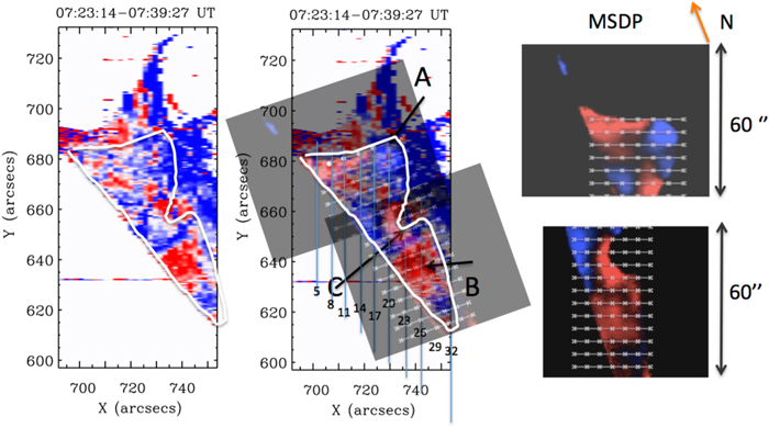
Figure 3. Coalignment of an IRIS Dopplergram and corresponding parts of MSDP observations are shown in the right panels. The left panel shows the IRIS Dopplergram overlaid by the Hα prominence contour. The middle panel shows the result of the coalignment. The white crosses, which are inside the contour of the Hα prominence, are the 75 pixels chosen for the comparison with IRIS data. The vertical lines indicated by numbers between 5 and 32 to show a sample of slits along which we selected the pixels corresponding to the 75 white crosses. We selected the nearest IRIS spectra corresponding to each MSDP pixel. The arrows A, B, and C point to the three different parts of the prominence that have different Doppler shift characteristics.
Download figure:
Standard image High-resolution image
Figure 4. Hα representative profiles of fifteen pixels among the 75 pixels indicated in Figure 3. The unit is in 10−6 erg s−1 cm −2 sr−1 Hz−1.
Download figure:
Standard image High-resolution image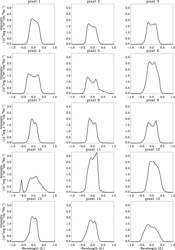
Figure 5. Mg ii k profiles corresponding to the 15 Hα profiles presented in Figure 4. The unit is in 10−7 erg s−1 cm −2 sr−1 Hz−1.
Download figure:
Standard image High-resolution image3. Spectroscopic Results
3.1. Mg ii h and k Lines: Ratio of Integrated Intensities
The integrated intensities of Mg ii h and k lines in each pixel of six rasters observed by IRIS between 07:06 UT, and 08:46 UT have been computed, encompassing a total of 192 spectra. To study the relationship between the Mg ii h and k line integrated intensities, we first selected the pixels which correspond to the prominence, and the disk in each spectra. We note that the maximum integrated intensity values of Mg ii k line (EMg ii k) are 35 × 104 erg s−1 cm−2 sr−1 in the disk, and only 8 × 10⁴ erg s−1 cm−2 sr−1 in prominence. Because the first raster image data is noisy, we calculate the ratio of the integrated intensities between the Mg ii h and k lines only from the remaining five rasters. In Figure 6 we show the results for the disk and the prominence. The mean values of the Mg ii h and k integrated intensity ratios are 1.36, and 1.39, respectively, for the disk and the prominence. The ratio for the disk is slightly lower than for previous observations of the mean quiet Sun chromosphere (1.45 in Lemaire et al. 1984). They are nevertheless higher than flare ratios, which are around 1 (Lemaire 1984; Kerr et al. 2015). Recently, low Mg ii k/h ratio was found also in the region on the disk close to the limb, i.e., in spicules where the value is 1.22 ±0.04 (Alissandrakis et al. 2018). Such values indicate a relatively optically thick regime (Leenaarts et al. 2013). In the case of prominences, the value of 1.39 fits well with the ratio already found in different prominences (Schmieder et al. 2014b; Liu et al. 2015; Levens et al. 2017; Jejčič et al. 2018). In an optically thin regime far above the limb, the ratio could increase and reach 1.96 (Kerr et al. 2015; Alissandrakis et al. 2018).
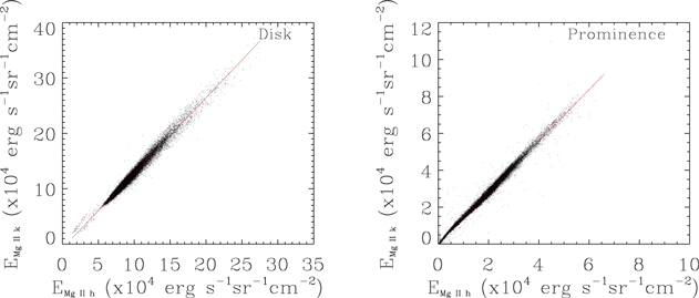
Figure 6. Examples of the variation of Mg ii k integrated intensity vs. Mg ii h integrated intensity for the disk, and prominence inside the field of view of IRIS rasters (second to sixth raster).
Download figure:
Standard image High-resolution image3.2. Mg ii h and k Lines: FWHM
We separate the prominence into two areas, one visible in both Mg ii and Hα lines (Prominence 1) and one visible only in Mg ii lines (Prominence 2) (Figure 7). To do so, we use a mask defined by the contour of the Hα intensity above a minimum threshold (Figure 1). We explore the FWHM in these two areas. The FWHM is computed by two methods presented in Paper I: the FHWM obtained by fitting the line wings of Mg ii k line with a single Gaussian which is the common shape of the observed profiles and a proxy of the FWHM derived by the quartile method. In Paper I, only one raster has been studied and one example of comparison has been shown. In a first approximation, both methods give compatible results (Paper I). Here, we statistically compare results from five rasters using all spectra in the Prominences 1 and 2. Normalized histograms are presented in Figure 8 for both areas. We see a systematic shift in the histograms between the results of the two methods, of the order of 0.1 Å for Prominence 1 and even more around 0.15 Å for Prominence 2. The single Gaussian fit neglects the secondary peaks in the line profiles while the quartile method already captures them, which explains why the profiles seem larger with that method. In Prominence 1, where the Hα prominence is visible, the two histograms are symmetrical and very few profiles are narrow. On the contrary in Prominence 2 prominence contour the Gaussian fit detects a maximum of narrow profiles. The broad profiles could be either a result of the sum of profiles of unresolved structures with a large dispersion of LOS velocities as we have shown with a test in C ii lines (see Paper I) or due to the large optical thickness of the plasma along the LOS (Jejčič et al. 2018).
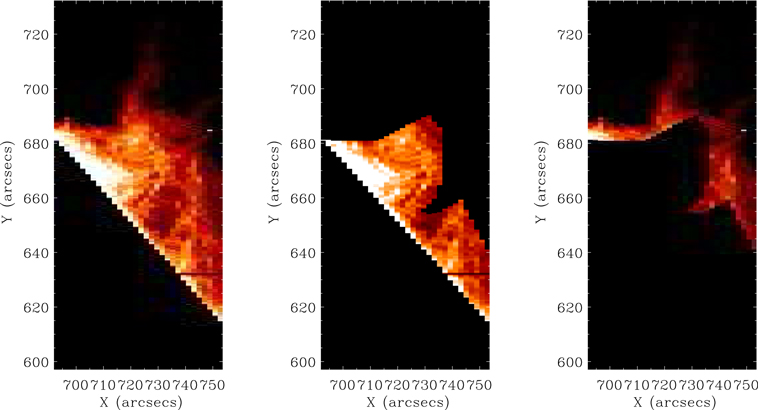
Figure 7. Left panel: the integrated intensity map of prominence in Mg ii observed with IRIS. Middle and right panels: we define a mask corresponding the contour of the Hα prominence in Figure 1. The middle panel shows (in Mg ii line) the part of the prominence which is visible also in Hα (Prominence 1), and the right panel shows the prominence which is not visible in Hα (Prominence 2).
Download figure:
Standard image High-resolution image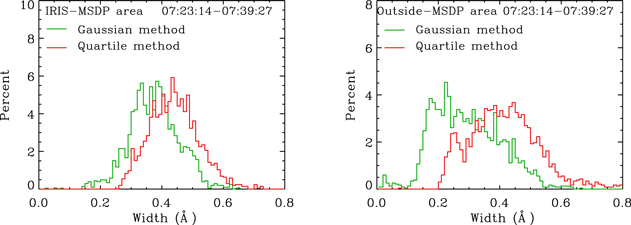
Figure 8. Examples of FWHM-normalized histograms obtained for the second raster of IRIS in the Mg ii k line for Prominence 1 visible in Hα (left panel) and for Prominence 2 not visible in Hα (right panel). In each panel the green line corresponds to the single Gaussian fit method, and the red line corresponds to the quartile method. The y unit represents the percentage of each individual rectangle area of the histogram divided by the integrated area limited by the curve which is equal to 1.
Download figure:
Standard image High-resolution image3.3. Mg ii k Line: Optical Thickness in Prominence 1 and Prominence 2
We compute the integrated intensity of Mg ii lines k and h, respectively, in Prominence 1 and Prominence 2. Figure 9 presents the ratio between integrated intensities of Mg ii h and k line versus the integrated intensity of Mg ii k in Prominence 1 (left panels) and Prominence 2 (right panels).
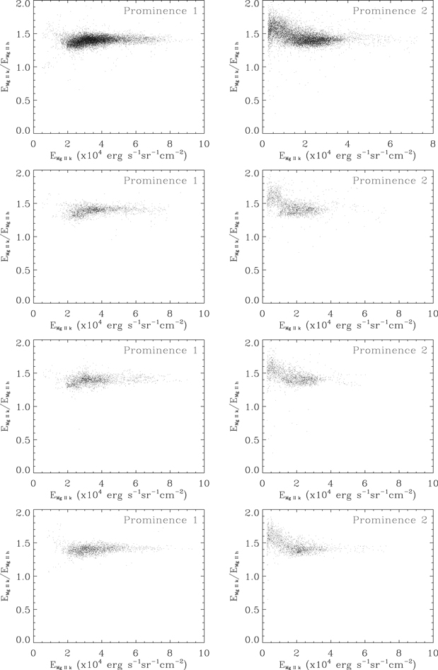
Figure 9. Relationship between the ratio of integrated intensities (Mg ii k vs. Mg ii h) and the Mg ii k integrated intensity for Prominence 1 visible in Hα (left column) and Prominence 2 not visible in Hα (right column). The first row panels correspond to the sum of pixels of five rasters (second to sixth raster), remaining raws to pixels of the second, third, and fourth raster, respectively.
Download figure:
Standard image High-resolution imageFrom this figure we can see that for Prominence 1 the integrated intensity values  are up to 8 × 10⁴ erg s−1 cm−2 sr−1 with a mean value around 3.5 × 10⁴ erg s−1 cm−2 sr−1. The optical thickness of Mg ii k for values around 3.5 × 10⁴ erg s−1 cm−2 sr−1 is between 15 and 100 according to the Figure 16 in Jejčič et al. (2018). For a slightly higher value than the mean value (EMg ii k = 5×10⁴ erg s−1 cm−2 sr−1), for which the optical thickness of Mg ii k may reach 1000 for a temperature of 6000 K. For Prominence 2 the mean integrated intensity values EMg ii k are around (2–2.8) × 104 erg s−1 cm−2 sr−1, for which the optical thickness of Mg ii is between 3 and 10. We summarized these values in Table 1. Similar results can be deduced from the theoretical study of 1D models with PCTR in Levens & Labrosse (2019). We conclude that there is a large difference of optical thickness for Mg ii k line between Prominence 1 visible also in Hα and Prominence 2 not visible in Hα.
Table 1. Optical Thickness of the Mg ii k-line (τMg iik) as Function of the Observed Integrated Intensity (EMg iik) Using the Grid of Models Fitting Mg ii Lines of Jejčič et al. (2018) and the Present Grid of Models Fitting Hα
| Prominence | EMgiik | τMg ii k | τMg ii k |
|---|---|---|---|
| erg s−1 cm−2 sr−1 | Models Fitting Mg ii | Models Fitting Hα | |
| Prominence 1 | 3.5 × 10 4 | 15–100 | 3–200 |
| visible in Hα | |||
| Prominence 2 | 2–2.8 × 10 4 | 3–1 0 | ⋯ |
| not visible in Hα |
Download table as: ASCIITypeset image
3.4. Mg ii h and k Lines: Ratio of the Integrated Intensities in Prominence 1 and Prominence 2
In Figure 9 (left panels), the ratio between integrated intensities of Mg ii h and k shows a large dispersion of the values between 1.3 and 1.5 for Prominence 1. This is consistent with the mean value (1.39) obtained by considering all the points (see Section 3.1). It is also the typical variation that was presented for other observed prominences (Jejčič et al. 2018; Levens & Labrosse 2019). Besides, in Prominence 2 the cloud of the points has an enhancement for the low values of  reaching 1.8 then decreasing to the normal mean values. We put a threshold for the very low values (2 × 10³ erg s−1 cm−2 sr−1) to eliminate the tail of the low ratios caused by the noise in the background. This decrease is found in the theoretical models (Jejčič et al. 2018). All of the values of the ratio of intensities of Mg ii h and k are consistent with the theoretical work of Jejčič et al. (2018), assuming a temperature in the prominence lower than 10,000 K. It will give a strong constraint for the conclusion of this paper (see Section 5).
The shape of the slope of the general distribution of the points in Figure 9 (right panels) corresponds to a microturbulence velocity of 5–8 km s−1 according to the plots in Jejčič et al. (2018).
3.5. Characteristics of Hα and Mg ii Profiles
Here, we focus on the characteristics of the Hα and Mg ii line profiles in Prominence 1 visible in both lines.
The FWHM of Mg ii profiles has been presented in Section 3.2. Figure 10 presents the FWHM of Hα in normalized histograms. Here we use 67 positions, removing eight positions where FWHM is not computable. To compute FWHM of the Hα line, we correct it for the instrumental profiles (see Paper I). By using the grating at zero-order, it is possible to get directly images of the MSDP slits defining the channels after the first pass. The resulting instrumental profile is close to a rectangle with the width of 0.18 Å. However, to correct the Hα FWHM, we use at first approximation the assumption that the Hα profile and the instrumental profile are Gaussian functions, thus obtaining  .
.
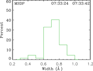
Figure 10. Example of FWHM-normalized histogram of the Hα profiles in the 75 pixels shown in Figure 3. The y unit represents the percentage of each individual rectangle area of the histogram divided by the integrated area limited by the curve, which is equal to 1.
Download figure:
Standard image High-resolution imageWe compute the integrated intensity EHa and EMg ii k for all 75 positions. From Figure 4 it is clear that the Hα profiles obtained by MSDP do not reach zero intensities in the wings. To assess the error due to the limited spectral range (±0.6 Å), we compare the obtained integrated intensities in two cases, the first one corresponds to the limited spectral range and the second to profiles with wings extrapolated to zero intensity. The differences between both integrated intensities is typically only 4 %.
The values of EHa corresponding to values of EMg ii k are presented in Figure 11 (red crosses). There is a certain relation between EHa and EMg ii k. EMg ii k is already saturated at around (2–3) × 104 erg s−1 cm−2 sr−1. EHa becomes saturated at values larger than 105 erg s−1 cm−2 sr−1 (Heinzel et al. 1994) because the Hα line is not so optically thick as the Mg ii k line. Therefore, the emission in Hα is due to the integration along the LOS of more structures than the Mg ii emission. In Section 4.2 we show the good correspondence of the observed variation EHa versus EMg ii k with the theoretical models.

Figure 11. Integrated intensity emitted in Mg ii k vs. integrated intensity of Hα for observations in Prominence 1 and grid of isothermal-isobaric models. Top panel for microturbulence 8 km s−1, bottom panel for microturbulence 16 km s−1.
Download figure:
Standard image High-resolution image4. NLTE Models and Comparison with Observations
Simultaneous prominence observations in the Hα, Mg ii h and k lines are quite unique (see Heinzel et al. 2015), and thus deserve certain attention from the modeling point of view.
4.1. Models
In this paper, we start with simplest 1D prominence-slab models (Labrosse et al. 2010; Heinzel 2015), where the prominence is represented by the slab of a finite thickness standing vertically above the solar surface. The slab is externally illuminated by the solar-disk radiation which sets the boundary conditions for the NLTE radiative transfer. We used the same NLTE code Multi-level Accelerated Lambda Iteration (MALI) as in Heinzel et al. (2014) and Jejčič et al. (2018). In this version of the code we used the diluted disk radiation incident on both sides of the vertical 1D slab for both Mg ii h and k lines, taken at a mean height of 13,000 km above the solar surface. The actual dilution factor (for the definition, see Jejčič & Heinzel 2009) is somewhat lower than 1/2 and only weakly dependent on the height. This height was derived from available prominence images. The input parameters of the 1D isothermal-isobaric slab are the kinetic temperature T, gas pressure p, geometrical (effective) thickness D, microturbulent velocity vt and the height of the observed structural element above the solar surface. For a given microturbulent velocity we computed large grid of 294 models for temperature ranging between 6000 and 20,000 K, gas pressure between 0.01 and 0.5 dyn cm−2, and a thickness between 200 and 5000 km. These ranges of values are commonly accepted for prominences (Labrosse et al. 2010). The MALI code solves the multi-level NLTE problem for a five-level plus continuum hydrogen atom and then for a five-level plus continuum model of Mg ii–Mg iii, using the partial redistribution approach for all resonance lines. The synthetic spectra are then obtained, among others, for the hydrogen Hα line and Mg ii h and k lines, to be compared with our observations. We use a common 1.5D inversion strategy, i.e., for each position (pixel) within a 2D prominence structure we try to fit the observed spectra using 1D slab models.
4.2. Synthetic Spectra
In Figure 11 we show the comparison between synthetic and observed integrated line intensities for both Mg ii k and Hα lines (note that here we show all 75 observed points as red triangles and all 294 models as blue dots). The fit between observed and computed intensities looks very promising and we find the following trend: while the Hα intensity increases, the Mg ii k one is more or less saturated in the range of observed intensities, indicating a large optical thickness of the Mg ii lines (see Table 2 in Heinzel et al. 2014). As shown by Gouttebroze et al. (1993) and Heinzel et al. (1994), Hα is optically thin for E(Hα) < 105 erg s−1 cm−2 sr−1, which is roughly the case of our observations. At larger intensities, Hα becomes optically thicker and starts to saturate. The computations were done for two distinct values of the microturbulent velocity, 8 and 16 km s−1, for reasons discussed below.
As we see from the histogram of observed Hα line widths, the FWHM reach up to 0.75 Å, which is sensibly larger than the modeled values. On the other hand, typical microturbulence in quiescent prominences does not exceed 5–8 km s−1 (see also Jejčič et al. 2018). Therefore, we first tried to fit the Hα line profiles and integrated intensities setting vt = 8 km s−1. Although the MSDP spectra have rather limited wavelength range of −0.6 Å to +0.6 Å on average, which leads to some uncertainties in determination of the FWHM and namely of the integrated intensity E(Hα), we used rather restrictive fitting criteria for Hα, and namely

We tried to find the best fit for Hα alone within such an accuracy, using 75 observed positions (pixels) where both Hα and Mg ii lines were visible. As a result, about one third of pixels does not exhibit any reasonable fit, while the remaining ones show a good fit. For them we constructed a histogram of prominence temperatures shown in Figure 12, top panel. It is not very surprising that such a fitting of large FWHMs leads to a dominance of high temperatures, up to our considered limit 20,000 K where we get the maximum on the histogram. We made various tests to get lower temperatures, either by introducing a PCTR (so that the central temperature of the slab could be decreased), or a plane-of-sky filling factor which accounts for a lower spatial resolution of MSDP. However, the histograms of the temperature still exhibited a significant number of points with high temperatures reaching 20,000 K.
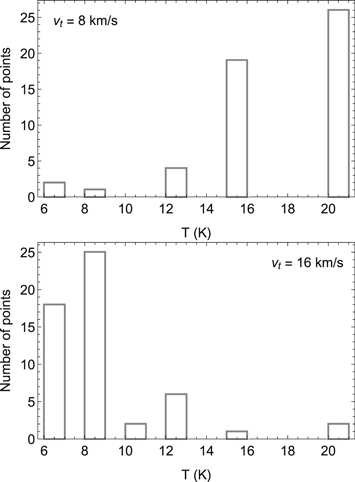
Figure 12. Distribution of temperature for isothermal-isobaric models based on the Hα profiles using two values of microturbulence: 8 and 16 km s−1
Download figure:
Standard image High-resolution imageBecause such temperatures are not typical for quiescent prominences (e.g., Tandberg-Hanssen 1995), we looked for another possibility to enhance FWHM of Hα and still keep temperatures at reasonable values. A natural way is to consider random LOS motions of prominence fine structures as in 2D multi-thread models of Gunár et al. (2008) where the hydrogen lines were modeled. However, in case of Mg ii lines, the appropriate MALI2D code for multi-threads is not yet fully available and thus we used a rough approximation that the LOS random motions can be treated as an additional "turbulence." We therefore arbitrarily increased vt to 16 km s−1. Then fitting again the Hα line we obtained much better temperature distribution as shown in Figure 12 (bottom panel) where the kinetic temperature peaks around 8000 K. For the increased microturbulence, the synthetic integrated intensity of Mg ii is also somewhat increased as can be seen from Figure 11 (bottom panel). Mg ii line absorption profile is significantly broadened by the microturbulence (for heavy ions the thermal broadening is much smaller) and, as a consequence, more radiation is absorbed within the reversal of the solar incident profile. This enhances the line source function and thus also the synthetic intensity. The effect is negligible for Hα as also seen from the correlation plots. One way to escape from this problem would be to run the MALI codes with vt = 8 km s−1 to get more realistic line source functions and only at the end compute the synthetic profiles with higher microturbulence. This could better simulate expected random LOS velocities. However, our ultimate goal is to perform 2D multi-thread modeling as was done for hydrogen by Gunár et al. (2012).
4.3. Electron Density, Gas Pressure, and Optical Thickness
The electron density which comes from hydrogen ionization (helium ionization is neglected here) and the gas pressure ranges are typical for quiescent prominences (Figure 13). Within the accuracy of 10%, the FWHMs and integrated intensities of Hα are also well reproduced (Figure 14). Next we show the distribution of the integrated Hα intensity as function of the Hα line-center optical thickness for fitted points (Figure 15). Nearly all such points have τ > 0.05 which seems reasonable for having a visible prominence in Hα. Only three points have τ lower and they correspond to low intensity profiles. Using these models we compute the optical thickness of Mg ii k and plot the integrated line intensities as function of τ (Figure 15). Comparing these values with the range that we derive in Section 3.3, using 1D models from Jejčič et al. (2018), we find a good agreement. Finally, the correlation plot between the line-center optical thickness of the k-line and that of Hα shows that the k-line can be up to a factor 100 thicker (Table 1).
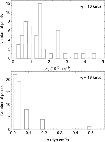
Figure 13. Top panel: distribution of electron density and Bottom panel: distribution of gas pressure for isothermal-isobaric models based on the Hα profiles using a microturbulence of 16 km s−1.
Download figure:
Standard image High-resolution image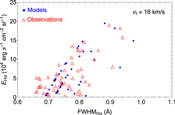
Figure 14. FMHW of Hα profiles for isothermal-isobaric models based on the 75 observed Hα profiles.
Download figure:
Standard image High-resolution image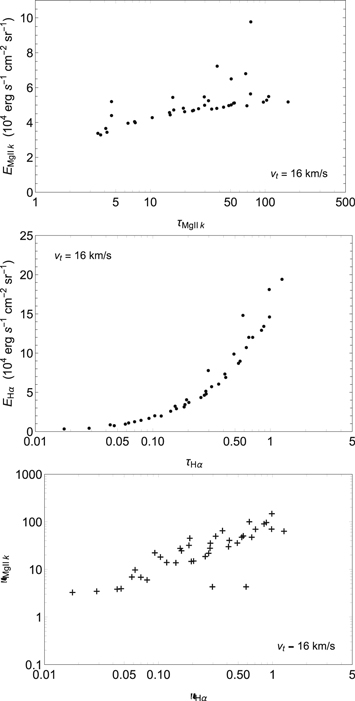
Figure 15. Top to bottom panels: integrated intensity emitted in Mg ii k vs. Mg ii k optical thickness, integrated intensity emitted in Hα vs. Hα optical thickness, optical thickness of Mg ii k line vs. optical thickness of Hα according to isothermal-isobaric models based on the 75 Hα profiles.
Download figure:
Standard image High-resolution image
5. Discussion and Conclusion
In this paper we analyzed a unique data set of coordinated prominence observations obtained both in the Hα line (by the MSDP on the Meudon solar tower) and in the Mg ii h and k lines (obtained by IRIS). We focused on statistical comparison of the integrated intensity and the FWHM between observations and synthetic spectra produced by 1D NLTE models which are isothermal and isobaric.
Observed FWHM of the Hα line are fitted with FWHM synthetic profiles. The mean value of the observed Hα width is around 0.7 Å. Fitting such broad profiles with 1D NLTE models naturally leads to large temperatures (up to 20,000 K) when a standard microturbulent velocity of 8 km s−1 is assumed. As an alternative solution to the problem of large Hα widths, we have considered significantly enhanced microturbulence, adopting a value of 16 km s−1. This particular prominence is very dynamic (see Paper I) and by assuming a large microturbulence we simulate the effect of random LOS motions of prominence fine structures. The used large microturbulence enhances the mean nonthermal velocity which leads to an additional Doppler broadening. Note that a similar approach was used by Alissandrakis et al. (2018) in the case of solar spicules. By introducing a large microturbulence into the 1D NLTE models we obtained models with reasonable temperatures, densities and pressures. In Figure 11 we show both the case with the enhanced microturbulence and the case with high temperatures. Although the results obtained by assuming the enhanced microturbulence may seem to be less satisfactory, this is an artifact of assuming an isotropic distribution of nonthermal velocities. Such a distribution leads to the turbulent Doppler brightening in Mg ii lines (see Section 4.2). Without such a brightening the pattern of both panels in Figure 11 would be similar. To reproduce the values of Hα FWHM, one could also consider the effect of the opacity broadening, i.e., a line saturation due to a high optical thickness. However, as it is clear from the observed Hα integrated intensities, the line-center optical thickness of Hα must be lower than one because EHα is lower than 105 erg s−1 cm−2 sr−1 (Heinzel et al. 1994). In such conditions of low optical thickness, the opacity broadening does not play any role.
The question then arises of why the Mg ii line intensities are statistically similar for the two cases of cool (around 8,000 K) and much hotter (20,000 K) plasmas. This looks counterintuitive taking into account that at 20,000 K, Mg ii gets highly ionized, forming Mg iii ion (Heinzel et al. 2014). However, even though the optical thickness of Mg ii k and h lines is substantially reduced due to the ionization of Mg ii, sufficient amount of Mg ii ions remains to produce integrated intensities similar to those produced at significantly lower temperatures. From Table 1, we can see that the optical thickness of Mg ii k line is between 3 and 200, while the optical thickness of Hα is between 0.05 and 2.
To decide which of the presented scenarios better represents the conditions of the observed prominence, we use an independent temperature constraint offered by the ratio of integrated intensities of Mg ii h and k lines. The ratios k/h derived from the observed data used in the present work have a mean value around 1.39 but can reach up to 1.8 in places with low integrated intensities (see Section 3.5). These values are consistent with previous results obtained by Jejčič et al. (2018; see their Figure 19), who show that the mean value of the line ratio below 1.5 corresponds to temperatures lower than 10,000 K. This result is only weakly dependent on the value of microturbulent velocity. Using this rather robust constraint, and the fact that the studied prominence is very dynamical and thus consistent with an assumption of fast unresolved motions, we conclude that the solution with lower temperatures and high microturbulence better represents the observations.
In future, we plan to extend the 2D multi-thread prominence fine structure modeling of Gunár et al. (2008), which assumes random LOS velocities of individual fine structures, to include also radiative transfer calculations in Mg ii lines. This will allow us to perform similar statistical analysis of simultaneous spectral observations as in Gunár et al. (2010, 2012), but including the IRIS Mg ii observations. The 2D multi-thread models are significantly more complex and currently in the development stage for Mg ii. However, by using models with random LOS velocities of individual fine structures, we will eliminate the need of large values of microturbulent velocity which only approximate the motions of fine structures. Multi-thread models will also more consistently resolve the issue of significantly different values of optical thickness of Hα and Mg ii h and k lines. The Mg ii lines are optically thick and thus convey information only from the structures nearest to the observer in the line core, but line wings are formed in the entire structure. On the other hand, the Hα line is relatively optically thin and thus samples different, deeper layers of observed prominences. However, in case of multi-thread models, even the optically thick Mg ii lines sample also the structures deeper in the prominence, if these structures move with LOS velocities different than structures in front of them. In such a case, due to the Doppler shift of individual intensity and opacity profiles and the narrow nature of Mg ii h and k lines, contribution to the total observed intensity comes from many layers.
G.P.R. and Y.C. acknowledge the support by the NNSFC grants U1831107, 41774180, 41331068, 11790303(11790300), Provincial Natural Science Foundation of Shandong (grant No. ZR2018MA031) to SDUWH, the CSC scholarship and the Key Laboratory of Solar Activity of the Chinese Academy of Sciences (CAS) under the grant number KLSA201602. S.J. acknowledges the financial support from the Slovenian Research Agency No. P1-0188. S.J., P.H., and S.G. acknowledge the support from the Czech Funding Agency through the grant No. 19-17102S. P.H. and S.G. acknowledge the support from grant No. 19-16890S of the Czech Science Foundation (GAČR). S.G. thanks for the support from project RVO:67985815 of the Astronomical Institute of the Czech Academy of Sciences and the financial support from the Observatoire de Paris through its "Postes Temporairement Vacants" programme during his visit at LESIA. G.P.R. thanks the LESIA at the Observatoire de Paris to welcome her having one year Chinese fellowship. We are grateful to Hui Tian for his IRIS codes for calibration. We thank SDO/HMI, SDO/AIA and IRIS science teams for the free access to the data. We are grateful to the observers at the Meudon solar tower (Regis Lecocguen and Daniel Crussaire).