
Displaced Harmonic Oscillator V ∼ min [(x + d)2, (x − d)2] as a Benchmark Double-Well Quantum Model


1
Department of Physics, Faculty of Science, University of Hradec Králové, Rokitanského 62, 500 03 Hradec Králové, Czech Republic
2
The Czech Academy of Sciences, Nuclear Physics Institute, Hlavní 130, 250 68 Řež, Czech Republic
Quantum Rep. 2022, 4(3), 309-323; https://doi.org/10.3390/quantum4030022
Submission received: 25 July 2022
/
Revised: 13 August 2022
/
Accepted: 19 August 2022
/
Published: 24 August 2022
Abstract
:For the displaced harmonic double-well oscillator, the existence of exact polynomial bound states at certain displacements is revealed. The N-plets of these quasi-exactly solvable (QES) states are constructed in closed form. For non-QES states, the Schrödinger equation can still be considered “non-polynomially exactly solvable” (NES) because the exact left and right parts of the wave function (proportional to confluent hypergeometric function) just have to be matched in the origin.
Keywords:
displaced harmonic oscillators; matching-method solutions; quasi-exact and non-polynomial exact bound states; double-well–single-well transitionPACS:
03.65.Ge Solutions of wave equations: bound states; 02.30.Gp Special functions1. Introduction
In the traditional realistic applications of quantum mechanics one picks up a tentative one-dimensional potential in a way inspired, say, by the principle of correspondence. Subsequently, one solves the corresponding “user-friendly” (i.e., ordinary differential) bound-state Schrödinger equation
numerically, arriving at the acceptance or rejection of the model in dependence on the agreement or disagreement between the predictions and the measurements [1].
The task becomes simplified when the needs of the quantum phenomenology are met by a function which is analytic. Then it makes sense to restrict attention to the potentials which are exactly solvable (ES, [2]) or at least partially exactly alias “quasi-exactly” solvable (QES, [3]). Indeed, the “redundant” analyticity requirement may prove useful, e.g., when one treats the elementary Schrödinger Equation (1) as a mere methodical laboratory needed, say, during the study of supersymmetric systems [4].
Whenever a suitable ES or QES model is not available, people feel motivated to assign the solvability status also to some non-analytic models . Typically, these models are of the piecewise constant square-well type [5]. In applications, their decisive formal merit is that their bound-state wave functions can be defined, using the matching method, in terms of elementary trigonometric functions.
In between the analytic and non-analytic extremes one finds a few parity-symmetric models in which the analyticity is only broken in the origin. Under this assumption it was possible to assign the QES solvability status to the spatially symmetrized quartic anharmonic oscillator [6] or to the symmetrized sextic anharmonic oscillator [7].
In the non-polynomial exact solvability (NES) context the non-QES exact spectra and bound states of the parity-symmetric models proved obtainable, for a few parity-symmetric potentials, via the matching of their exact special-function left and right parts of the wave functions. This enabled one to assign the NES status to the symmetrized exponential potential (with expressed in terms of Bessel functions [8,9]), to its asymptotically decreasing alternative [10] and/or to the symmetrized Morse potential (i.e., to the sum of the two exponentials for which appeared proportional to a confluent hypergeometric function [11,12]).
In our present paper we intend to complement these results by showing that in some of the parity-symmetric quantum models and, in particular, for
in Equation (1), the QES and NES regimes can coexist. One might also add that disproportionately, the ES quantum systems with the single-well harmonic-oscillator potential is discussed in virtually any textbook on quantum mechanics (cf., e.g., [13]). In contrast, the most straightforward twinned, d-displaced generalization (2) of the harmonic-oscillator model with is never mentioned. In what follows, we intend to fill the gap.
1.1. Motivation in Physics
In the context of physics the above-mentioned NES constructions were motivated by the needs of molecular physics so that the non-analyticity of in the origin appeared inessential. Nevertheless, even in this area of physics the analyticity of the benchmark models re-emerged as essential, mainly due to the related possibility of a qualitative analysis of quantum dynamics using the mathematical tools of the classical theory of catastrophes [14].
The simplest forms of the theory (viz., the so called fold and cusp catastrophes) proved mostly needed [15]. Let us just remind the readers briefly that in this language the equilibrium of a classical dynamical system is identified with a minimum of a suitable “Lyapunov” potential [16]. This enables one to classify all of the qualitatively different patterns of the bifurcation of the equilibria in terms of the parameter-dependence of the minima.
By far the most interesting and useful example of such a bifurcation pattern is called cusp catastrophe. In this case one conventionally chooses
It is then easy to verify that such a Lyapunov function possesses a single minimum at but two minima (i.e., a double-well shape) at and at a not too large b. It is also worth noting that in the a-b plane the boundary of transition between the two regimes is a spiked, cusp-shaped curve [17]. Thus, one can use the formalism for a qualitative description of dynamics, say, of the Josephson junction between the two Bose–Einstein condensates [18].
After one turns attention to the genuine quantum forms of dynamics, the work with the classical a-b plane geometry of model (3) ceases to be satisfactory. One can expect that the classical bifurcation phenomena become smeared out by the quantization. In particular, in the double-well case, due to the tunneling, one would only have to move far away from the fine-tuned cusp singularity in order to be able to distinguish, experimentally, between the low-lying states which remain localized, in general, either near the left minimum or near the right minimum of .
In the latter, deep-double-well dynamical regime the tunneling becomes suppressed since the growth of the distance – between the minima becomes accompanied by their increasing separation mediated by a growing and thickening barrier [19]. The approximate calculation of the bound states may be then facilitated by the use of a fairly efficient local harmonic-oscillator approximation,
More or less equivalently, one may replace by a global double-well harmonic oscillator,
Whenever the difference or becomes large, the low-lying states remain localized just near one of the minima. The realization of a genuine quantum effect of bifurcation may only be expected to occur when and . Thus, we arrive at the spatially symmetric toy-model potential
in which we may scale out and obtain the ultimate double-well version of the one-parametric potential (2) of our present interest.
1.2. Motivation in Mathematics
At the not too large displacements d, the elementary one-dimensional potential (2) can be perceived as an example of a smooth perturbation of an ubiquitous harmonic oscillator. Still, the non-analyticity of in the origin looks “suspicious”. For this reason, in spite of the relative boundedness of the perturbation, the model seems to never be recalled in the context of perturbation theory. It sounds almost like a paradox in that in the textbooks on quantum mechanics the role of the most popular illustrative example of the perturbation of harmonic oscillator is almost invariably played by the (nicely analytic) quartic harmonicity ∼ yielding the vanishing radius of convergence of the resulting Rayleigh-Schrödinger perturbation series [20].
In our recent comment on quartic anharmonicities [6] we pointed out that the not too rational (perhaps, purely emotionally motivated) insistence of the major part of the physics community on the strict analyticity of the one-dimensional phenomenological potentials did also cause problems in the monograph [3]. Indeed, the author of this very nice review of the so called quasi-exactly solvable (QES) Schrödinger equations (offering also an extensive list of further relevant references) did not imagine that besides the best known sextic-polynomial QES potential , the QES status can be also assigned, in a way explained in [6], to its quartic-polynomial predecessor, provided only that we admit its non-analyticity at .
Recently we returned to the QES problem and imagined that even the quartic polynomials which were studied and assigned the QES status in the latter reference need not still represent the “first nontrivial” case. Our subsequent study of the problem resulted in the conclusion that the role of the simplest nontrivial QES quantum model can in fact be played by the spiked harmonic oscillator (2).
A concise constructive demonstration of this assertion is to be presented in the following section.
2. Polynomial Solvability
Our model (2) is important as it offers a qualitative description of the phenomena connected with the changes of the topology of the forces as characterized by the so called pitchfork bifurcation of equilibria in classical mechanics [16]. In quantum context Formula (2) interpolates between the exactly solvable limit (yielding the doubly degenerate spectrum of energies , , where the superscript marks the parity of the related wave functions) and another exactly solvable limit providing the same, but non-degenerate, spectrum of energies , with parities . In between the wave functions have to be derived as satisfying the physical boundary conditions in infinity as well as in the origin.
2.1. The Matching of States in the Origin
The phenomenological appeal of the genuine quantum bifurcations often forces us to turn attention to approximate methods. Pars pro toto let us mention our recent studies [19,21] of the phenomenon of tunneling in which an analytic (in fact, polynomial) potential possessing an N-plet of the local minima , has been replaced, in the low-lying spectrum regime, by a locally adapted harmonic-oscillator well as sampled, at , by Equation (4). Beyond the harmonic-oscillator approximation as well as beyond , the construction of the wave-functions using the matching of the logarithmic derivatives at the -plet of non-analyticities becomes purely numerical.
In this sense our present toy model is exceptional. At any (i.e., not necessarily just at bound-state) energy E its exact and correct wave functions (which vanish in infinity and could be called, therefore, the Jost solutions) are proportional to certain special functions which can be considered known (see their explicit form given a bit later below). Thus, one only has to match the logarithmic derivatives of the resulting left branch and right branch of in the origin,
As long as the ultimate, properly matched wave function has to be of an even or odd parity, we may write with or , respectively. Thus, under certain non-singularity conditions in the origin we may introduce an arbitrary regular ad hoc normalization
and arrive at the two alternative “shooting method” matching rules
In this spirit also the above-cited samples of a few other NES constructions of bound states can be perceived as the implementations of the same matching rules alias transcendental Equation (8). In all of these cases, these equations determine the whole spectrum of the bound state energies in an implicit manner.
2.2. The Simplest Polynomial Solution
Our interest in one-dimensional potential (2) was born when we noticed that it is quasi-exactly solvable (QES). By definition [3] this means that it admits the existence of exact elementary wave functions at certain parameters and energies. One can easily verify, by insertion, that at a special shift the nodeless function
belongs to , obeys the standard matching conditions (i.e., has a continuous logarithmic derivative in the origin) and satisfies our Schrödinger Equations (1) + (2) at exactly. Thus, this expression represents the even-parity ground-state wave function of the model.
A non-constructive proof of the QES property of our model is elementary. In the single-well scenario we choose the special value of and inserted the nodeless function
(which belongs to ) in Schrödinger equation
Clearly, function (10) obeys the standard matching conditions in the origin (i.e., it has a continuous logarithmic derivative there) and it solves our bound-state problem (2) + (11) at . Thus, QES expression (10) represents the exact even-parity ground-state wave function. In Figure 2 our QES choice of parameters has been used for illustration purposes. The similar elementary QES feature also occurs after one moves to the double-well dynamical regime.
Let us add that in the standard literature the QES property has only been assigned to the 1D potentials which were manifestly analytic along the whole real line [22,23,24,25,26,27,28]. The present, non-analytic generalization of the QES property has only been proposed in Ref. [6]. The non-analytic QES construction has been preformed there for the phenomenologically important class of quartic anharmonic oscillators. Our present real QES wave function (10) may be also recalled as providing a closed-form illustration of the fact that besides the potential, also our wave functions are non-analytic at since
We are persuaded that the descriptive merits of the similar generalized QES constructions overweight their not too essential feature of non-analyticity at . In this sense the existing literature would certainly deserve to be completed.
2.3. Systematic Approach
After one inserts potential (2) in Schrödinger Equation (11) it is possible to assume the existence of the even-parity and/or odd-parity QES bound-state solutions in the most general form of the standard normalizable polynomial ansatz such that, on the positive half-axis,
We may accept the normalization convention
With and after appropriate insertions and elementary algebra the QES solvability of the model appears equivalent to the validity of the set of linear recurrences
From the last item with we get the QES value of energy so that we are left with an N-plet of relations between the unknown coefficients , , …, and an unknown, QES-compatible value (or rather a multiplet of values) of the shift .
Starting from the choice of and we find that the odd solution cannot exist while the well known even-parity solution only exists at . In the next step with and the single constraint only admits the pure harmonic oscillator in the odd-parity case while the first nontrivial QES solutions with emerges in the even-parity scenario.
Once we skip the harmonic-oscillator solutions and demand that we may set and in Equation (15). Then we have to satisfy the set of two relations
This leads to the two easy odd-parity solutions with and . They become accompanied by the equally easy even-parity solutions with and .
Next we choose and find that the odd-parity construction degenerates to the triplet of relations
with solution , and . In parallel, the even-parity conditions
lead to the slightly less trivial quadruplet of eligible QES shifts
Each one of them defines the related two coefficients
2.4. General Case
At any N we may study the QES sets of coupled nonlinear algebraic equations using the computer-assisted elimination technique of Gröbner bases. In the even-parity case this algorithm generates certain polynomials which specify the QES-compatible shifts d as their zeros (see Table 1). The odd-parity QES solutions appear determined, similarly, via the values of which coincide with the real zeros of other polynomials (see Table 2).
The most compact representation of the above set of results may be obtained when one imagines that the even- and/or odd-parity boundary condition (14) at may be reinterpreted as the respective initial, additional (i.e., ) condition for recurrences (15). This enables us to solve these recurrences in terms of compact formulae.
Theorem 1.
In the even-parity QES case the general closed-form solution of recurrences (15) reads
Its d-dependence is encoded in the tridiagonal k by k matrices
These formulae must be complemented by the constraint , i.e., by the polynomial algebraic equation
which represents an implicit definition of all of the admissible values of the specific, QES-compatible shift parameters .
Proof.
One may proceed by mathematical induction. It is only necessary to keep in mind that in matrix (20) the first row reflecting the initial condition looks (and is) anomalous. That is why the form and validity of the solution and also of the solution are to be verified separately. □
Theorem 2.
In the odd-parity QES case the closed-form solution of recurrences (15) reads
with the d-dependence encoded in the tridiagonal k by k matrices
This must be complemented by the algebraic polynomial-equation definition , i.e.,
yielding all of the admissible values of the specific, QES-compatible shift parameters .
Proof.
Once one keeps in mind that in the odd-parity cases we have at all N and k, the proof remains elementary and proceeds, along similar lines as above, by mathematical induction. □
3. Special-Function Solvability
In the broader context of quantum physics, the amount of attention which is currently paid to polynomially solvable (traditionally called “exactly solvable”, ES) Schrödinger equations seems disproportionate. Especially in comparison with the fact that the attention virtually disappears in the NES cases, i.e., immediately behind the latter ES area. The paradox is striking because the sophisticated commercial software (such as MAPLE or MATHEMATICA, etc.) as well as the freely available NIST review [29] enable the physicists to work with elementary functions as easily as with the special functions.
Within the NES approach one can decide to treat the terminating and non-terminating confluent hypergeometric series on equal footing. As an immediate consequence of such an amendment of the paradigm one obtains an extension of the class of the user-friendly interactions. In our present paper we accept the idea and intend to describe one of its most natural implementations in the one-dimensional quantum-dynamical scenario.
In this context one can feel inspired by the classical Thom’s concepts of stability and of its loss which are closely related to the algebraic geometry of the minima of certain analytic Lyuapunov’s functions [30]. For this reason the classical dynamics near a cusp-related bifurcation (i.e., near an “abrupt” transition between one and two stable minima of ) is traditionally described via a representative analytic, anharmonic-oscillator (AHO) polynomial (3). It is widely believed that the polynomial Lyapunov’s functions are best suited for the study of the Thom’s classical catastrophes and that even the constructions of their quantum analogues should not break the correspondence with these polynomials. Thus, even though our present model could have also pretended to play the role of a cusp-related Lyapunov function (especially in the simplest nontrivial bifurcation scenario with in AHO model), it seemed disqualified by its non-analyticity in the origin.
3.1. Single-Well Dynamical Regime with
Very recently we imagined that any quantization of a classical catastrophe must replace the usual schematic time-dependent trajectories in a classical space of states by certain selfadjoint operators in a suitable infinite-dimensional physical Hilbert space [31,32,33]. Thus, after quantization the concepts such as bifurcation (etc.) must necessarily be transferred from the domain of algebraic geometry to the area of functional analysis and spectral theory. Naturally, this implies that the non-analyticity of becomes inessential while its solvability may start playing the role of a significant merit in comparison with a purely numerical nature of AHO Schrödinger equations [34,35,36,37]. In other words, the twinned harmonic oscillator (2) with a variable real displacement d and with two minima if seems suitable and acceptable as a benchmark quantum model with catastrophic features.
Besides the serendipitous and rather formal QES property as discussed above, a turn of attention to the fully general twinned harmonic-oscillator model (2) is recommended from a phenomenological perspective. Another independent reason would be again mathematical. After an elementary change of variables one reveals that Equation (1) coincides with the two branches of the confluent hypergeometric equation which are matched together in the origin. In this sense our model (1) + (2) resembles square wells and remains solvable via the matching of logarithmic derivatives of at . In the literature the conceptual appeal of the complete and, in principle, arbitrarily precise solvability based on the use of confluent hypergeometric special functions may be found advocated by multiple authors [1]. In what follows we will defend and accept such an NES point of view, demonstrating its applicability to the one-parametric family of potentials (2) in both of their one-centered and two-centered realizations.
Once we recall the left-right symmetry (i.e., parity-symmetry, -symmetry) of our Hamiltonian, we may temporarily restrict our attention to the differential Equation (1) on one of the half-lines (i.e., say, with ). Then we may change variables as follows,
Whenever we choose a negative , this converts Equation (1) into Kummer’s equation
(cf. [29], §13.2(i)) with parameters and . As long as we may ignore the branch-point singularity of Equation (25) at and we may write down the general solution as a superposition of two independent confluent hypergeometric series, viz.,
and
Subsequently, we have to satisfy the asymptotic physical boundary condition. This forces us to combine the two independent solutions and of Equation (25) in the following unique manner,
The choice of this function with the power-law asymptotical behavior valid in the complex plane of with the left cut from to yields the correct, asymptotically vanishing wave functions at positive in closed form,
The formula remains manifestly dependent on the value of energy E. After the matching of the left and right branches of our analytic solution in the origin, the spectrum of bound states will be obtained as split in the even-parity and the odd-parity states. Their energies will coincide with the roots of the respective transcendental secular equations, viz.,
or
Here the prime marks the derivative with respect to the first argument.
The numerical performance of the determination of the energies based on the latter equations is entirely routine and reflects our expectations that with the growth of the negative shift the narrowing of the potential well will push the energy levels upwards. Thus, the standard HO ground state with the energy equal to one will be pushed up to with and (this is quasi-exact state), etc. The similar accelerated growth moves the second excited state from initial more quickly to , etc. The bracketing property of the latter type of results is highly welcome in computations of course.
3.2. Double-Well Dynamical Regime with
In the double-well regime with positive the presence of the square-root branch-point of Equation (25) at , i.e., inside the interval of physical coordinates would make the direct use of the asymptotically correct closed-form solutions (28) slightly uncomfortable. The key new technicality is that one must keep the choice of the proper branch of the coordinate function under explicit control.
For this reason we recommend the use of an alternative bound-state construction in which one recalls the -symmetry of our Schrödinger Equation (1) and employs a variant of the so called shooting method. In the language of mathematics this means that one simply separates the spatially even wave functions (for which we set and as an initial boundary condition) from the spatially odd solutions (for which we have and )—this is to be compared with Equations (30) and (31), respectively. In each of these two subcases one arrives again at the Kummer’s Equation (25) which is now defined in an extended and partially doubly covered interval of and .
In contrast to preceding subsection we will now solve the initial-value alias Cauchy problem knowing that we know its general solution in confluent-hypergeometric form
In the next stage of development we fix the ratio of the coefficients via the above-mentioned initial conditions imposed upon the both-sided limits of and at (i.e., at when taken below its square-root branch). The subsequent necessary control of the choice of the branch of function (27) (i.e., of the analytic-function component of our solution (32) at ) is not difficult because we have (i.e., a square-root branch) in definition (27).
In the last step we may finally recall the standard oscillation theorems [38] which
- relate the quantum number of a bound-state energy to the number of the finite nodal zeros of ;
- enable us to perturb , localize the related maximal real (and, say, positive) finite nodal zero and find the one-to-one correspondence between the exact-bound-state-energy limits of and of .
The latter correspondence enables us to localize, numerically, the exact energy, with arbitrary preselected precision, via a trial-and-error choice of , to be iteratively amended by a tentative, smaller and smaller decrease (whenever the maximal real node keeps growing) or increase (whenever the maximal node happens to leave the real line and become complex).
4. The Displacement-Dependence of the Spectrum
The numerical results of the above-outlined algorithm are sampled in Figure 3 and by Table 3, Table 4 and Table 5. The key advantage of such a special-function-based version of the well known shooting algorithm is that in our model the trial-and-error functions are known in the exact (albeit rather clumsy, computer-stored) special-function confluent-hypergeometric form (which is closed and analytic but, unfortunately, still too long for a printed display). This enables us to keep the numerical errors under active control and to construct, systematically, the pairs of the lower and upper estimates of the bound-state energies.
In Table 3 sampling the ground-state results, the non-monotonicity of the dependence of the energy is slightly counterintuitive but still easy to understand. It is obvious that the growth of the positive shift leads, at the beginning, to the broadening of the well without a significant change of its size near the origin. This implies the possibility of an approximation of the potential by a broader effective well, i.e., in a solvable approximation, by with yielding the smaller ground state energy. Later, i.e., at the larger shifts d the central repulsive spike starts growing more quickly, separating the two HO wells and making them only weakly coupled. This must lead, approximately, to the double degeneracy of the low-lying spectrum and, in particular, to the unavoidable return of the ground state energy to its initial value at the sufficiently large ds.
Table 4 illustrates that as long as the wave function of the first excited state vanishes in the origin, it is much less sensitive to the influence of the central spike. According to our tests, the energy just decreases with the growth of d and, in contrast to the behavior of the ground state energy, it never drops below at the large shifts . Marginally we may add that the test is facilitated by the observation that at the relevant spectral bound , the wave-function solutions with the correct odd-parity behavior in the origin may be further simplified and expressed in terms of error functions. This simplification of the general solution also facilitates the demonstration of the complex-value nature of the asymptotic nodal zero at any .
5. Conclusions
In conclusion, let us re-emphasize that in the current literature there exists a large number of papers and studies devoted to the experiments and realistic models of quantum physical systems described by a simplified, one-dimensional (i.e., ordinary differential) Schrödinger equation (i.e., often, by our Equation (1) which is defined on the whole real line of the coordinate). Still, in contrast to the dominance of the scene by the papers describing the bound states lying in a single-well potential, one finds perceivably less papers dealing with the potentials having a double-well shape. Naturally, one of the reasons is purely formal. One often finds that many methods of solving Schrödinger equations (and, among them, the perturbation-expansion methods) happen to fail when applied to the double-well systems.
This leads to a remarkable conflict between the prevailing, purely mathematically motivated preference of the single-well models in various methodical considerations, and the frequently encountered lack of some sufficiently efficient construction recipes, especially in the context of the double-well scenarios which are much more interesting, in the phenomenological context, mainly due to the emerging manifestations of the influence of the tunneling effect.
In such a context we sought, in our present paper, for a nontrivial support of the existing tendencies towards an extension of the class of the “exactly solvable” 1D potentials from their completely analytic subset to its non-analytic generalizations. We are persuaded that such a tendency is natural and well motivated. We also believe that in the nearest future our approach might find some immediate and successful applications, e.g., during some of the popular and, usually, partially non-numerical descriptions of the physical systems (as studied, e.g., in [39]) in which, in the language of mathematics, the double-well structure of the potential is necessary, but in which the phenomenon of the avoided level crossing is expected to occur while being not so easily detected by the mere finite-precision experimental measurements of the spectra.
Last but not least let us mention that among the physical systems to which our present methodical innovation could also appear, in the nearest future, to be immediately applicable are also, potentially, all of the various more-dimensional realistic multi-well models as encountered, e.g., in quantum chemistry [40] and/or in the quantum-computation-motivated mesoscopic physics of the systems of quantum dots [41]. Indeed, under the widespread interaction-analyticity constraint, just the approximate solutions of the partial differential Schrödinger equations are usually available in these systems.
In the methodical context, a strengthening and/or independent complement of our present arguments may be also found in Ref. [11] where we sampled the methodical as well as practical gains of the approach by introducing a spiked, centrally symmetrized 1-D potential of the Morse-oscillator type. In spite of its non-analyticity in the origin the model was still shown to exhibit several features of the more conventional complete exact solvability.
For the similar and generic 1-D interactions characterized by the various incomplete forms of solvability (such as QES) the situation appears mathematically more complicated because the presence of the non-analyticities at some coordinates may restrict, severely, the practical as well as methodical applicability of the incomplete constructions in quantum physics. One can feel encouraged by the existence of parallels between the one-dimensional and three-dimensional central interactions. The phenomenological appeal of the latter models is usually perceived as independent of the presence or absence of a non-analyticity in the origin. Pars pro toto, let us just mention the singular nature of the so-called shape-invariant realizations of supersymmetry in quantum mechanics [2].
There are no reasons for an asymmetric treatment of solvability (and, in particular, of the QES models) in one and three dimensions. As long as in 3-D models the singularities in the origin are currently tolerated, a transfer of the same “freedom of non-analyticity” to 1-D systems is desirable. In our present paper we showed that such a change of paradigm is also productive (new models may be constructed) and satisfactory (in the QES setting, the classification of models may be formulated as starting from the most elementary quadratic polynomials).
After a removal of the QES constraints, the next-to-elementary, NES nature of our present bound-state problem (1) + (2) can be perceived, on a purely methodical level, as an inspiration of possible piecewise-analytic shifts, matchings and generalizations of many other traditional phenomenological interactions. Even if we restrict attention just to the present example (2) offering a tunable transition between a single- and double-minimum shape, we would like to emphasize that it possesses several specific advantages.
First of all, the exact analytic form of the related NES wave functions offers an undeniable amendment, e.g., in comparison with the conventional polynomial options as sampled by the famous Mexican-hat (MH) central potential
Thus, one of the domains of possible applicability of our model (2) might be sought in the advanced field theories of self-interacting systems possessing the so called Nambu-Goldstone bosons in which the use of benchmark remains popular in spite of its purely numerical nature (cf., e.g., picture Nr. 7 in [42]). Not insisting too much on the analyticity of , the author of loc. cit. emphasized that with , the MH dynamical ansatz leads to the solutions which “have lower symmetry than the Lagrangian, and contain mass zero bosons”.
We believe that in comparison with , our present model could prove competitive, in spite of its non-analyticity, not only in the above-mentioned area but also in various more straightforward applications ranging from the elementary quantum mechanics of atoms and molecules up to various topics in condensed matter physics. In all of these areas the possible phenomenological use of our NES quantum model (1) + (2) might complement the purely numerical approaches which are needed when the currently more popular polynomial potentials are used.
Funding
This research received no external funding.
Institutional Review Board Statement
Not applicable.
Informed Consent Statement
Not applicable.
Data Availability Statement
Not applicable.
Conflicts of Interest
There is no conflict of interests.
References
- Flügge, S. Practical Quantum Mechanics I; Springer-Verlag: Berlin, Germany, 1971. [Google Scholar]
- Cooper, F.; Khare, A.; Sukhatme, U. Supersymmetry and quantum mechanics. Phys. Rep. 1995, 251, 267. [Google Scholar] [CrossRef] [Green Version]
- Ushveridze, A.G. Quasi-Exactly Solvable Models in Quantum Mechanics; IOPP: Bristol, UK, 1994. [Google Scholar]
- Witten, E. Dynamical breaking of supersymmetry. Nucl. Phys. B 1981, 188, 513. [Google Scholar] [CrossRef]
- Quesne, C.; Bagchi, B.; Mallik, S.; Bila, H.; Jakubsky, V.; Znojil, M. PT-supersymmetric partner of a short-range square well. Czech. J. Phys. 2005, 55, 1161. [Google Scholar] [CrossRef] [Green Version]
- Znojil, M. Symmetrized quartic polynomial oscillators and their partial exact solvability. Phys. Lett. A 2016, 380, 1414–1418. [Google Scholar] [CrossRef] [Green Version]
- Quesne, C. Quasi-exactly solvable symmetrized quartic and sextic polynomial oscillators. Eur. Phys. J. Plus 2017, 132, 450. [Google Scholar] [CrossRef]
- Znojil, M. Symmetrized exponential oscillator. Mod. Phys. Lett. A 2016, 31, 1650195. [Google Scholar] [CrossRef] [Green Version]
- Sasaki, R. Confining non-analytic exponential potential V(x)=g2exp(2|x|) and its exact Bessel-function solvability. arXiv 2016, arXiv:1611.02467. [Google Scholar]
- Sasaki, R.; Znojil, M. One-dimensional Schroedinger equation with non-analytic potential V(x)=−g22exp(−|x|) and its exact Bessel-function solvability. J. Phys. A Math. Theor. 2016, 49, 445303. [Google Scholar] [CrossRef] [Green Version]
- Znojil, M. Morse potential, symmetric Morse potential and bracketed bound-state energies. Mod. Phys. Lett. A 2016, 31, 1650088. [Google Scholar] [CrossRef] [Green Version]
- Sasaki, R. Symmetric Morse potential is exactly solvable. arXiv 2016, arXiv:1611.05952. [Google Scholar]
- Messiah, A. Quantum Mechanics; North Holland: Amsterdam, The Netherlands, 1961. [Google Scholar]
- Thom, R. Structural Stability and Morphogenesis. In An Outline of a General Theory of Models; Benjamin: Reading, UK, 1975. [Google Scholar]
- O’Dell, D.H.J. Quantum Catastrophes and Ergodicity in the Dynamics of Bosonic Josephson Junctions. Phys. Rev. Lett. 2012, 109, 150406. [Google Scholar] [CrossRef] [PubMed] [Green Version]
- Zeeman, E.C. Cxatastrophe Theory-Selected Papers 1972–1977; Addison-Wesley: Reading, UK, 1977. [Google Scholar]
- Available online: https://en.wikipedia.org/wiki/Catastrophe_theory (accessed on 15 August 2022).
- Goldberg, A.Z.; Al-Qasimi, A.; Mumford, J.; O’Dell, D.H.J. Emergence of singularities from decoherence: Quantum catastrophes. Phys. Rev. A 2019, 100, 063628. [Google Scholar] [CrossRef] [Green Version]
- Znojil, M. Arnold’s potentials and quantum catastrophes. Ann. Phys. 2020, 413, 168050. [Google Scholar] [CrossRef] [Green Version]
- Arteca, G.A.; Fernández, F.M.; Castro, E.A. Large Order Perturbation Theory and Summation Methods in Quantum Mechanics; Lecture Notes in Chemistry; Springer: Berlin, Germany, 1990; Volume 53. [Google Scholar]
- Znojil, M.; Borisov, D.I. Arnold’s potentials and quantum catastrophes II. Ann. Phys. 2022, 442, 168896. [Google Scholar] [CrossRef]
- Singh, V.; Biswas, S.N.; Datta, K. Anharmonic oscillator and analytic theory of continued fractions. Phys. Rev. D 1978, 18, 1901. [Google Scholar] [CrossRef]
- Turbiner, A.V. Quasi-exactly solvable problems and sl(2) algebra. Commun. Math. Phys. 1988, 118, 467. [Google Scholar] [CrossRef]
- Fring, A. A new non-Hermitian E2-quasi-exactly solvable model. Phys. Lett. A 2015, 379, 873. [Google Scholar] [CrossRef] [Green Version]
- Fring, A. E2-quasi-exact solvability for non-Hermitian models. J. Phys. A Math. Theor. 2015, 48, 145301. [Google Scholar] [CrossRef] [Green Version]
- Znojil, M. Quasi-exactly solvable quartic potentials with centrifugal and Coulombic terms. J. Phys. A Math. Gen. 2000, 33, 42034211. [Google Scholar] [CrossRef] [Green Version]
- Znojil, M. Harmonic oscillator well with a screened Coulombic core is quasi-exactly solvable. J. Phys. A Math. Gen. 1999, 32, 4563. [Google Scholar] [CrossRef] [Green Version]
- Bender, C.M.; Boettcher, S. Quasi-exactly solvable quartic potential. J. Phys. A Math. Gen. 1998, 31, L273. [Google Scholar] [CrossRef]
- Available online: http://dlmf.nist.gov/13.7 (accessed on 15 August 2022).
- Arnold, V.I. Catastrophe Theory; Springer: Berlin, Germany, 1992. [Google Scholar]
- Znojil, M. Horizons of stability. J. Phys. A Math. Theor. 2008, 41, 244027. [Google Scholar] [CrossRef]
- Znojil, M. Quantum catastrophes: A case study. J. Phys. A Math. Theor. 2012, 45, 444036. [Google Scholar] [CrossRef] [Green Version]
- Lévai, G.; Ruzicka, F.; Znojil, M. Three solvable matrix models of a quantum catastrophe. Int. J. Theor. Phys. 2014, 53, 2875. [Google Scholar] [CrossRef] [Green Version]
- Bender, C.M.; Wu, T.T. Anharmonic oscillator. Phys. Rev. 1969, 184, 1231. [Google Scholar] [CrossRef]
- Turbiner, A.V.; Ushveridze, A.G. Anharmonic oscillator: Constructing the strong-coupling expansions. J. Math. Phys. 1988, 29, 2053. [Google Scholar] [CrossRef]
- Alvarez, G. Bender-Wu branch points in the cubic oscillator. J. Phys. A Math. Gen. 1995, 27, 4589. [Google Scholar] [CrossRef]
- Eremenko, A.; Gabrielov, A. Analytic continuation of eigenvalues of a quartic oscillator. Comm. Math. Phys. 2009, 287, 431. [Google Scholar] [CrossRef] [Green Version]
- Hille, E. Ordinary Differential Equations in the Complex Domain; Wiley: New York, NY, USA, 1976. [Google Scholar]
- Znojil, M. Avoided level crossings in quasi-exact approach. Nucl. Phys. B 2021, 967, 115431. [Google Scholar] [CrossRef]
- Znojil, M. Relocalization switch in a triple quantum dot molecule in 2D. Mod. Phys. Lett. B 2020, 34, 2050378. [Google Scholar] [CrossRef]
- Znojil, M. Polynomial potentials and coupled quantum dots in two and three dimensions. Ann. Phys. 2020, 416, 168161. [Google Scholar] [CrossRef] [Green Version]
- Goldstone, J. Field theories with superconductor solutions. Il Nuovo Cimento 1961, 19, 154. [Google Scholar] [CrossRef]
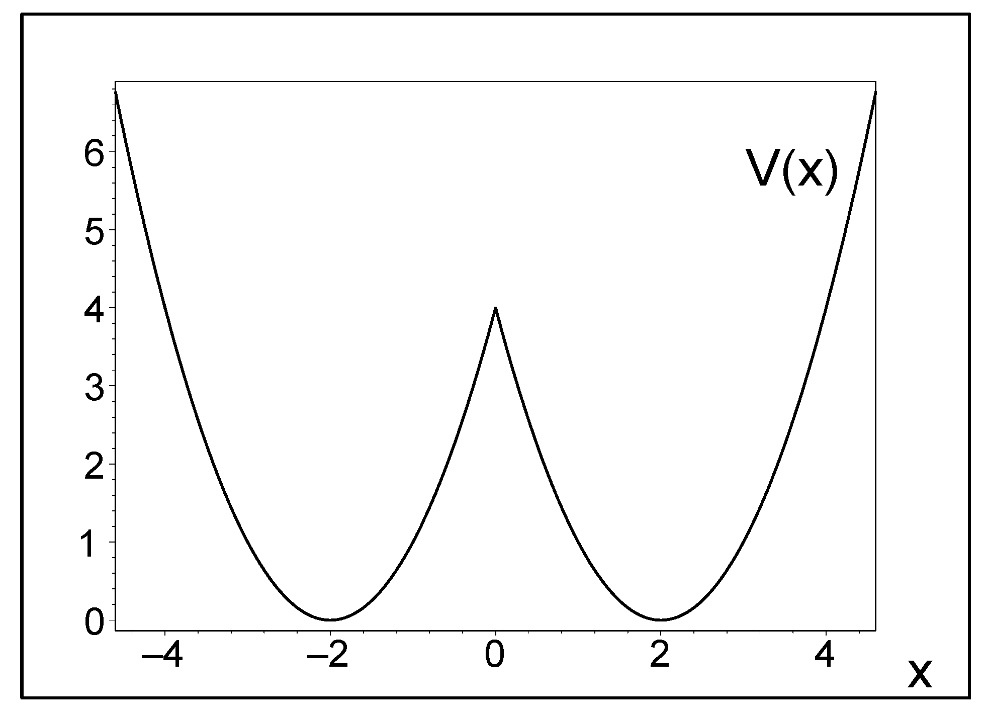
Figure 1.
Double-well shape of potential (2) at positive .
Figure 1.
Double-well shape of potential (2) at positive .

Figure 2.
Ground-state energy and wave function in the single-well QES version of potential (2) at .
Figure 2.
Ground-state energy and wave function in the single-well QES version of potential (2) at .

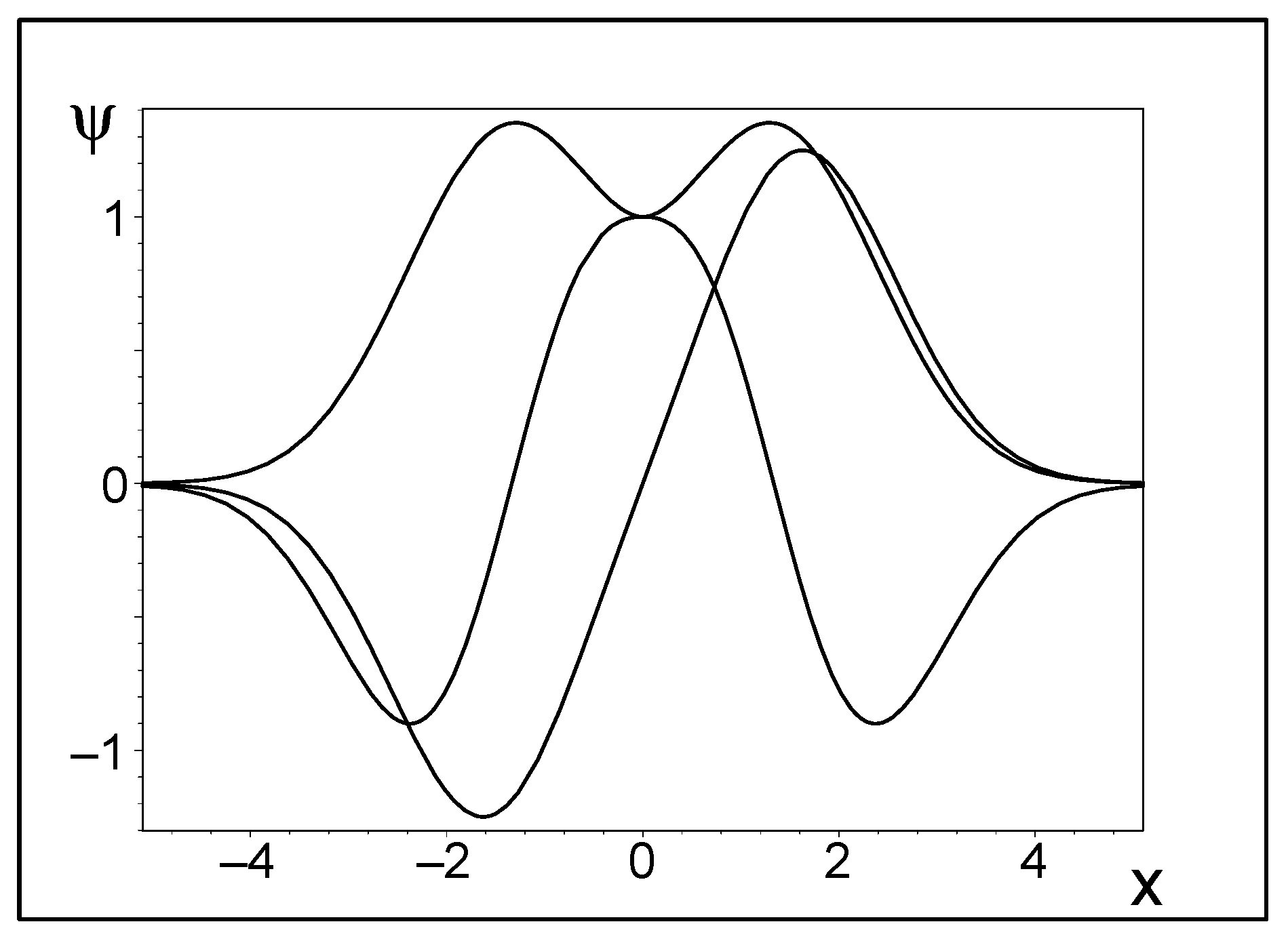
Figure 3.
The first three double-well wave functions at .


Table 1.
QES even-parity values of shifts d are defined, implicitly, as zeros of polynomials . A sample of the Gröbnerian elimination is added.
Table 1.
QES even-parity values of shifts d are defined, implicitly, as zeros of polynomials . A sample of the Gröbnerian elimination is added.
| N | Polynomial | Elimination of |
|---|---|---|
| 2 | ||
| 3 | ||
| 4 | ||
| 5 | ||
| ⋮ | … | … |
Table 2.
QES values determined as zeros of polynomials (odd-parity case).
| N | Polynomial | Elimination of |
|---|---|---|
| 2 | ||
| 3 | ||
| 4 | ||
| 5 | ||
| ⋮ | … | … |
Table 3.
The shift-dependence of the ground-state energy.
| Shift | Energy Estimates | |
|---|---|---|
| Lower | Upper | |
| 0 | 1 | 1 |
| 0.25 | 0.768972 | 0.768974 |
| 0.50 | 0.635528 | 0.635530 |
| 0.75 | 0.590300 | 0.590301 |
| 1.00 | 0.618910 | 0.618920 |
| 1.50 | 0.801493 | 0.801494 |
| 2.00 | 0.951410 | 0.951420 |
| ∞ | 1 | 1 |
Table 4.
The shift-dependence of the 1st-excited-state energy.
| Shift | Energy Estimates | |
|---|---|---|
| Lower | Upper | |
| 0 | 3 | 3 |
| 0.25 | 2.483910 | 2.483920 |
| 0.50 | 2.060760 | 2.060770 |
| 0.75 | 1.724710 | 1.724720 |
| 1.00 | 1.468460 | 1.468470 |
| 1.50 | 1.157479 | 1.157480 |
| 2.00 | 1.035760 | 1.035770 |
| ∞ | 1 | 1 |
Table 5.
Shift-dependence of the 2nd-excited-state energy (at the state is quasi-exact).
| Shift | Energy Estimates | |
|---|---|---|
| Lower | Upper | |
| 0 | 5 | 5 |
| 0.25 | 4.34600 | 4.34700 |
| 0.50 | 3.79410 | 3.79420 |
| 0.75 | 3.34470 | 3.34471 |
| 1 | 3 | 3 |
| 1.50 | 2.64860 | 2.64870 |
| 2.00 | 2.73500 | 2.73510 |
| ∞ | 3 | 3 |
Publisher’s Note: MDPI stays neutral with regard to jurisdictional claims in published maps and institutional affiliations. |
© 2022 by the author. Licensee MDPI, Basel, Switzerland. This article is an open access article distributed under the terms and conditions of the Creative Commons Attribution (CC BY) license (https://creativecommons.org/licenses/by/4.0/).
Share and Cite
MDPI and ACS Style
Znojil, M. Displaced Harmonic Oscillator V ∼ min [(x + d)2, (x − d)2] as a Benchmark Double-Well Quantum Model. Quantum Rep. 2022, 4, 309-323. https://doi.org/10.3390/quantum4030022
AMA Style
Znojil M. Displaced Harmonic Oscillator V ∼ min [(x + d)2, (x − d)2] as a Benchmark Double-Well Quantum Model. Quantum Reports. 2022; 4(3):309-323. https://doi.org/10.3390/quantum4030022
Chicago/Turabian StyleZnojil, Miloslav. 2022. "Displaced Harmonic Oscillator V ∼ min [(x + d)2, (x − d)2] as a Benchmark Double-Well Quantum Model" Quantum Reports 4, no. 3: 309-323. https://doi.org/10.3390/quantum4030022