
Comparison of J Integral Assessments for Cracked Plates and Pipes

1
Institute of Theoretical and Applied Mechanics of the Czech Academy of Sciences, v. v. i. Prosecká 809/76, 190 00 Prague, Czech Republic
2
Faculty of Mechanical Engineering, Czech Technical University in Prague, Technická 4, 166 07 Prague, Czech Republic
*
Author to whom correspondence should be addressed.
Materials 2021, 14(15), 4324; https://doi.org/10.3390/ma14154324
Submission received: 25 June 2021
/
Revised: 23 July 2021
/
Accepted: 27 July 2021
/
Published: 2 August 2021
Abstract
:The purpose of this article is to compare two predictive methods of J integral assessments for center-cracked plates, single-edge cracked plates and double-edge cracked plates produced from X52 and X70 steels, and a longitudinally cracked pipe produced from X70 steel. The two methods examined are: the GSM method and the Js procedure of the French RCC-MR construction code, designated here as the FC method. The accuracy of J integral predictions by these methods is visualized by comparing the results obtained with the “reference” values calculated by the EPRI method. The main results showed that both methods yielded similar J integral values, although in most cases, the GSM predictions were slightly more conservative than the FC predictions. In comparison with the “reference” values of the J integral, both methods provided conservative results for most crack configurations, although the estimates for cracks of a relative length smaller than 1/8 were not found to be so conservative. The prediction of burst pressures for external longitudinal semielliptical part-through cracks in X70 steel pipe showed that the magnitudes of predicted burst pressures came very close to each other, and were conservative compared to FEM (finite element method) calculations and experimentally determined burst pressures.
1. Introduction
The aim of this study was to demonstrate that the newly modified GS method [1], now renamed as GSM method, provides reliable J integral predictions which compare well with predictions based on the generally accepted Js procedure of the French RCC-MR construction code [2]. Before defining the problems concerned with these predictions it should be stated that the J contour integral, as proposed by Rice [3], has gained recognition as a fracture-characterizing parameter in elastic–plastic solids. Being based on an energy balance approach, it can also be used as an elastic–plastic energy release rate (under certain restrictions). J integral is still used widely in several state-of-the-art papers, e.g., [4,5,6]. Generally, the determination of the J integral for a cracked body loaded with a certain stress pattern is not simple and the solution of this problem requires, with the exception of some simple bodies and crack configurations, employment of computerized numerical methods. In some situations, the exact determination of the J integral may not be required. What may be required (or at least desirable), however is a simple method that can show, from the viewpoint of integrity, whether the exploited structural component containing a crack-like defect is still safe to continue operating. In such cases, a conservative estimate of the J integral could provide essential information on the integrity of a cracked body. A more precise (and therefore expensive) FEM analysis would then only be used when this conservative approximate analytical method predicts failure. Therefore the relevancy of the study can be seen in that the developed GSM method provides a good conservative estimation of the J integral for various cracked components.
In contrast to J integral computation, determination of the stress intensity factor K, as a fracture characterizing the parameters of brittle materials, is much simpler. Several compendia on stress intensity factors exist, e.g., Tada et al. [7], Rooke and Cartwright [8], and Murakami [9], which enable various crack problems to be solved in the area of linear elastic fracture mechanics. From the definition of the J integral, it is clear that this quantity is dependent not only on the stress pattern, size, and configuration of a crack (like it is for K) but also on the stress–strain relationship of the material of the body. This consequently indicates that there is some relationship between the J integral, the stress intensity factor, and the stress–strain dependence. Although several approximate methods have been proposed for the determination of this relationship, we have concentrated on two of them: the GSM method and the FC method. The latter method, proposed as early as 1985 in Addendum A16 of the French nuclear code [2] as the Js method, became a subject of further development and was then integrated into the 2007 edition of the RCC-MR code as published by Marie et al. [10]. In this edition, the correction factor in the plastic zone φ (according to the denotation used in this article) has been altered compared to the 1985 edition. Further development of the AFCEN Codes yielded the RCC-MX Code in 2008, and finally the RCC-MRx Code in 2018. As reported by Muňoz Garcia et al. [11], the 2018 code contains a set of technical rules to be applied in the design of research reactors. It should be stated that the general formalism for the Js integral is based on the reference stress concept introduced by Ainsworth [12].
2. Background of the GSM and FC Methods
2.1. The GSM Method
This method is based on (i) a formal description of the J integral for a circular notch from the definition, (ii) substitution of the relative strain energy density along the periphery of the notch by a third power of the cosine function of the polar angle, and (iii) allowing the radius of the circular notch to go to zero in the final expression for the J integral. The idea of a formal description of the J integral, for a circular notch followed by reducing the notch radius to zero in the final expression for obtaining the J integral of a crack, is not new. There are some papers by Matvienko and Morozov [13,14] and by Matvienko [15] which demonstrate such an approach.
As shown by Norio and Yasuhiro [16], stress intensity factors can be determined from the limiting values of elastic stress concentration factors as the root radius ρ of the notch approaches zero. In the derivation of the J integral, the GSM method considers a symmetrically loaded notch with its tip embedded in a mode I stress field. The maximum stress σmax occurs directly ahead of the notch. Dimensional considerations of the crack-tip stress field for an isotropic elastic body lead to:
According to the definition, the J integral for a cracked body is given by the expression
where
- is the strain energy density
- Γ is any contour encircling the tip of the crack in a counterclockwise direction
- Ti are the components of the traction vector
- ui are the displacement vector components
- ds is a length increment along the contour Γ
Let us consider a body with external notches on both sides, loaded perpendicularly to the plane of the notches. A section of the notched body around the notch is shown in Figure 1.
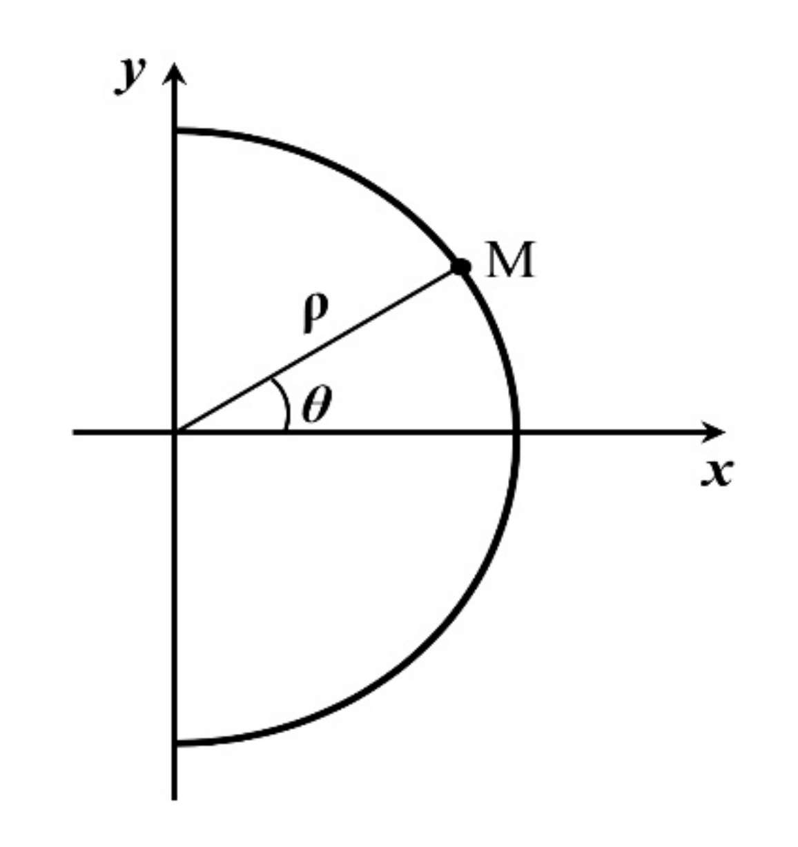
The shape of the notch root is semicircular, the radius being ρ. By the concept of the invariance of the J integral, the value of the J integral does not depend on the path of integration. In its derivation the J integral is formally written for the notched body, and the path of integration is chosen so as to coincide with the periphery of the semicircular notch root (see Figure 1). Since the path of integration leads over a free surface, the second term on the right-hand side of Equation (2) becomes zero, so that after the transformation of Cartesian to polar co-ordinates of the points on the semicircular notch root (Figure 2), the J integral for the notched body takes the form:
The GSM method relates the strain energy density w(θ) at point M on the periphery of the notch root, characterized by the polar angle θ, to the maximum strain energy density wmax = w(θ=0). The relation between w(θ) and wmax depends not only on the polar angle θ but also on the magnitude of the load. The results of finite element investigations into the strain energy density along a notch root in a double-edge notch panel [1] showed that the relative strain energy density (w(θ)/wmax) can be substituted with a certain approximation by the function cos3θ. Considering this, Equation (3) can be rewritten as:
The infinitesimal strain energy density dw is given in principal stresses and strains as:
In the notch root, characterized by θ = 0, the stress σ2 is always zero because of the free surface; the stress σ3 is zero for the plane stress state; and the strain ε3 is zero for the plane strain state. This means that the infinitesimal strain energy in the notch root (θ = 0) is reduced to
so that the strain energy density becomes
or, with the notation used before:
The GSM method supposes that material obeys the Ramberg–Osgood dependence (9) and that the hypothesis of equivalent strain energy density at the notch tip [17] can be applied:
According to the concept of this hypothesis, the following equation holds
where wn is the energy density due to the net section stress σn.
By combining (8) and (10), we arrive at:
By differentiating the Ramberg–Osgood relation (9), and considering that ε0 = σ0/E, it is possible to arrive at:
When applying this equation for εn and σn to Equation (11), the following expression for w is obtained:
By substituting wmax in Equation (4) with this expression, the J integral for a notch obtains the form:
Recalling Equation (1), it is seen that the stress intensity factor for a crack can be expressed by:
From there it follows as:
By combining Equations (14) and (15) we obtain:
A multiple of four/three is applied to the first term in expression (17); this does not have a theoretical basis, but was incorporated to provide a well-known form of the elastic component of the J integral: Jel = K2/E′, where E′ = E for plane stress and for plane strain, ν being Poisson´s number.
Equation (17) then obtains the form:
Since the strain energy density w(θ) in Equation (4) was substituted with wmax cos3θ regardless of whether plane stress or plane strain conditions were concerned, the resulting Formula (18) can be used as a basis for the J integral assessment at conditions of plane stress and plane strain. As is known, the EPRI estimation scheme for the J integral [18] comes from stresses given by the HRR singularity and it arrives at the relationship simply expressed as:
P0 can be defined arbitrarily, e.g., as the limit load PL. In order to make Equation (18) comply with this, a so-called limit load parameter C, by which the uniaxial yield stress σ0 in (18) is to be multiplied, is introduced into the GSM method. The C parameter is given by Equation (20):
Equation (18) then obtains the form:
The limit load PL in Equation (20) can be determined as the product of the yield stress σ0 and a certain geometrical function, which is specific for each panel and depends on the crack length a and the width b of a cracked panel of unit thickness. It is seen that the difference between the J assessment in the plane stress condition and in the plane strain condition is given (besides Young´s modulus E′) by the level of the limit load parameter C.
2.2. The FC Method
As already mentioned, the FC method was proposed in Addendum A16 of the French nuclear code [2] as the Js method, and its further development was published by Marie et al. [10]. The basis of this method was the R6 procedure [19], which made it possible to arrive at the following formula for the J calculation:
In Equation (22), Je is the elastic component of the J integral, εref is the reference strain corresponding to the reference stress σref defined by Equation (23), εe = σref/E is the elastic strain, and φ is the plastic zone size-correction factor given in [10] by Equation (24):
It can be pointed out that, owing to Equation (20), the reference stress σref can also be written as:
The first term in the brackets of Equation (22) reflects what experimentalists observed a long time ago, namely that at a certain load the J integral is proportional to the ratio of the actual strain to its elastic component. The quantities used in expression (22) are illustrated in Figure 3 for the Ramberg–Osgood approximation of the tensile curve of the material.
The Ramberg–Osgood dependence (9) can be rewritten by substituting σ with σref and ε with εref to obtain the form:
By denoting
and considering
Equation (26) obtains the form:
According to Equation (22), and considering Equations (24) and (28), the J integral is then expressed by Equation (29):
This type of equation is also used in later editions of the RCC-MR code. The very last edition from 2018, denoting the RCC-MRx code, is not readily available from public sources. As follows from [11], it has been designed primarily for the mechanical components of high-temperature structures of nuclear installations; however, it can also be used for mechanical components of other types of nuclear installations. Although not mentioned explicitly in [11], it is likely that an equation of the type in (29) is also used in the RCC-MRx code, at least for some specific conditions like force-imposed mechanical loading, the modified limit load basis for the reference stress, and the Ramberg–Osgood description of the stress–strain curve.
Coming back to Equation (29), the fraction in Equations (26) and (27) can be substituted, according to Equation (25), by to obtain
where
3. Use of the GSM and FC Methods for Cracked Plates
3.1. Description of Procedure
Before beginning to describe the procedure of comparing predictions using the GSM and FC methods, a few notes regarding the main way in which the GS method was modified, should be considered. It is worth noting that the first modification was made a few years ago when the so-called plastic constraint factor on yielding C′ was introduced to account for crack-tip constraint in cracked pipes from pipeline steels. On the basis of experimentally determined fracture pressures for part-through axial cracks of known dimensions, the C′ factor was found to vary between 2.0 and 2.4 for relative crack depths a/t ranging between 0.57 and 0.72 [20,21,22]. This enabled us to predict critical conditions for pipes containing deep part-through cracks. Owing to the limited group of steels tested and the narrow range of crack dimensions, there was a need for a more general approach to determine the J integral for various types of components. This is why the limit load concept was used in the GSM method instead.
For verification of the Formulas (21) and (30), it is necessary to compare the results calculated on the basis of these formulae with those obtained by exact calculations, mostly using finite-element analysis. The verification should be done for a wide range of crack sizes, component geometries, and loadings. However, in general, this requires versatile elastic–plastic computer programs. On the other hand, several simplified post-yield fracture mechanics methods, even if based on finite elements calculations, have been developed. Among these, the EPRI method [18] seems to be very convenient for the verification of the formulae derived, although it has been demonstrated in some papers that the EPRI method contains errors and inaccuracies in some of the J estimates. However, the EPRI method is easy to apply for simple component geometries and it utilizes the Ramberg–Osgood description of the stress–strain relationship of the material. It is widely used, so there is no need to describe it here.
With a view to test specimen configurations for which the EPRI method offers J integral solutions, the following specimens have been considered: (i) center-cracked panel (CCP), (ii) double-edge cracked panel (DECP), and (iii) single-edge cracked panel (SECP). These panels are shown schematically in Figure 4.
Since the plastic component of the J integral strongly depends on the strain hardening exponent n, it is advisable to consider materials with various n values. For this reason, two pipeline steels were taken into account: X52 and X70. These steels were manufactured by Mannesmann company, Siegen, Germany. The stress–strain curves for these steels, as approximated by the Ramberg–Osgood relationship, are shown in Figure 5. The Ramberg–Osgood parameters, as well as the magnitudes of the U.T.S. for these steels are presented in Table 1.
The procedure for the verification of the GSM and FC methods consists in several steps. Firstly, it is necessary to determine the limit load parameter C according to Equation (20) for each type of specimen (panel) in both the plane stress and plane strain condition. The limit loads for the specimens used in the investigation can readily be found in various publications, e.g., [23,24]. They are recapitulated here:
CCP specimen
DECP specimen
SECP specimen
where
The results of transforming these limit loads to the limit load parameters C for CCP, DECP, and SECP specimens are shown in Table 2.
In the next step, the stress-intensity factors K are determined. For this purpose, the handbook [7] cited earlier is used. For the specimens used, the formulae for the K determination have the common form
where σ is gross section stress and the function is specific for each type of specimen: i.e., fCCP for CCP specimens, fDECP for DECP specimens, and fSECP for SECP specimens. The mathematical notations for these functions are the following:
Knowing the magnitudes of the limit load parameter C and the magnitudes of the stress-intensity factor K, the J integrals can be calculated by the GSM and FC methods using Equations (21) and (30) with (31). As it is more convenient in the comparison of the two investigated methods to use gross section stress σ instead of the net section stress σn, it is necessary to transform σn to σ in Equations (21), (30) and (31).
3.2. Results of Calculations
3.2.1. The Center-Cracked Panel (CCP)
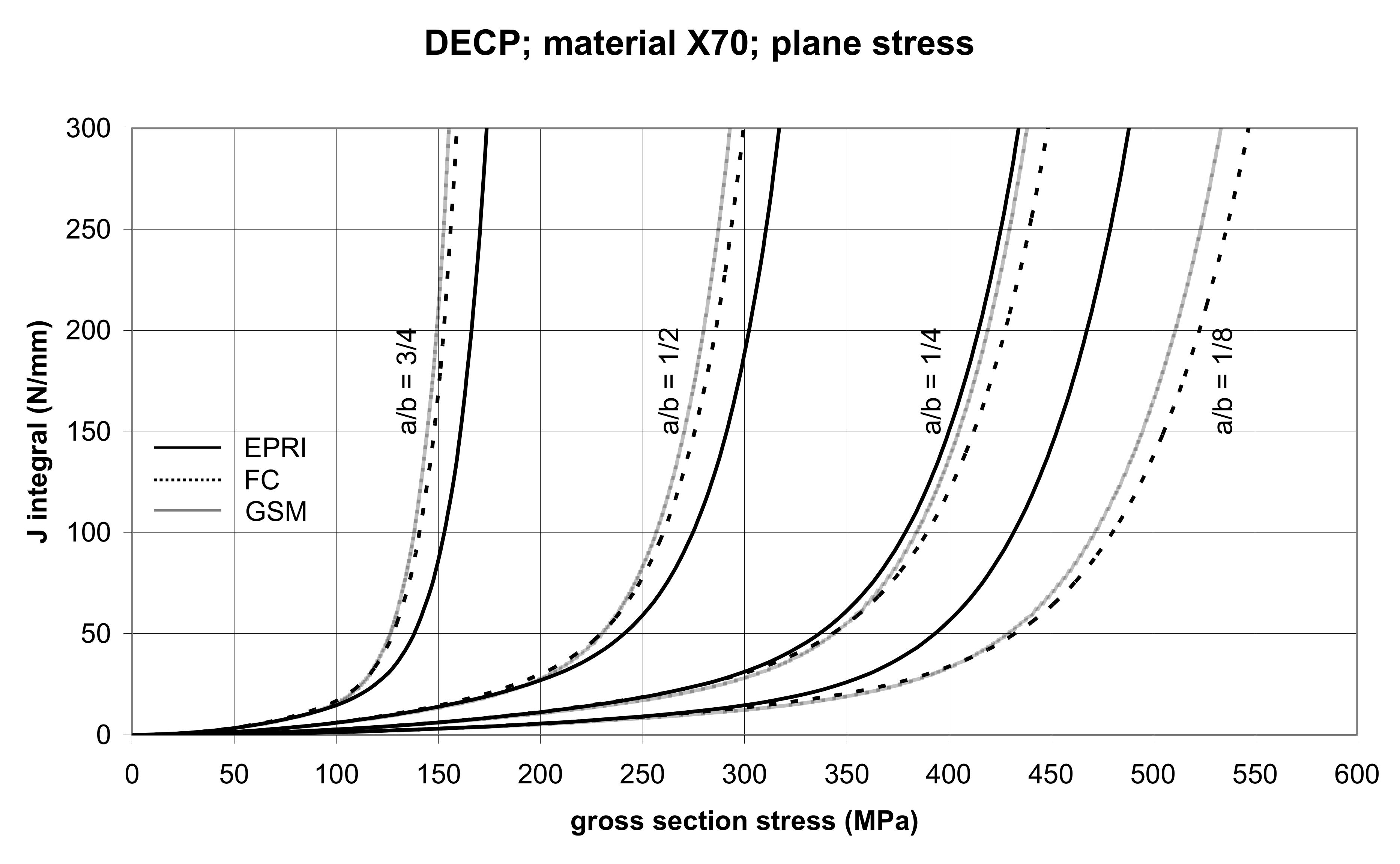
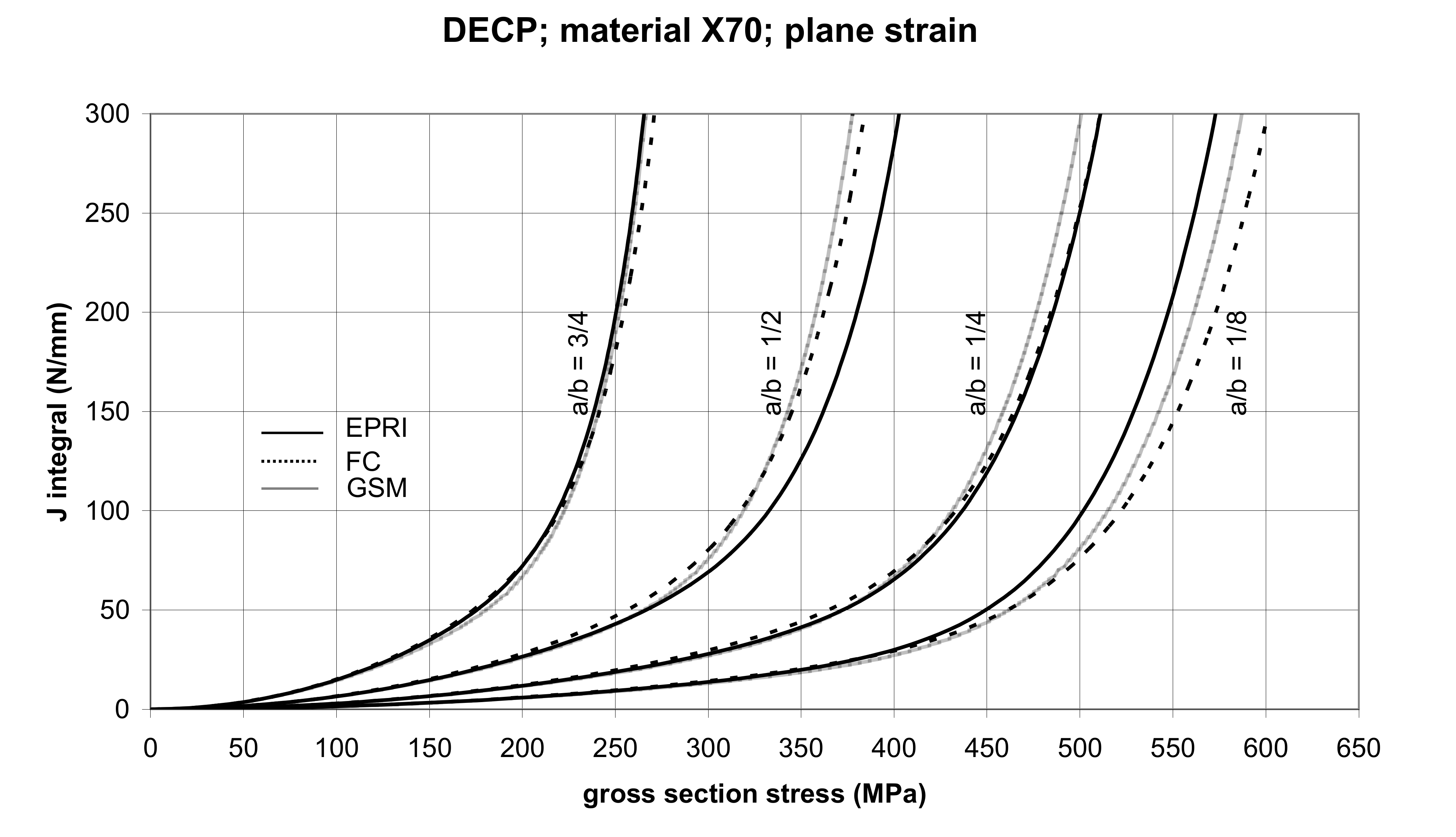
3.2.2. The Double-Edge Cracked Panel (DECP)
3.2.3. The Single-Edge Cracked Panel (SECP)
4. Use of the FC and GSM Methods for Cracked Pipes
4.1. Preparation of Pipe Segment
The verification of simplified engineering methods is best when conducted on real cracked components. Simplified methods, such as the FC and GSM methods, can be used, e.g., in the assessment of the integrity of pressure gas pipelines. They can be damaged by corrosion defects at the outside surface when corrosion protection fails [25]. The technical state of gas pipelines is therefore periodically assessed. This becomes increasingly significant when the planned lifetime of gas pipelines is close to expiring [26]. It is then necessary to increase the frequency of inspections of pipelines to identify in time the most dangerous of defects in pipelines—cracks. In order to evaluate critical conditions for a crack (crack size, gas pressure), it is very important to assess the J integral as the fracture-characterizing parameter and compare it with the fracture toughness Jm of the pipe material.
For this purpose, we conducted tests on a segment taken from a gas pipeline made from X70 steel, measuring 1018 mm in outside diameter and 11.7 mm in wall thickness. The effective length of the pipe segment (the distance between the welds in dished bottoms) was approximately 3.5 D, where D was the outside diameter. A ring approximately 300 mm long was also cut from the pipeline to manufacture specimens for testing the mechanical and fracture-mechanical properties of the pipe material.
The tensile specimens were orientated circumferentially, and orientation of the CT specimens was such that crack-starter notches were axial. A curved semiproduct from the ring was press-straightened and then used to manufacture flat specimens for tensile tests. The tensile properties, namely the yield stress σY = σ0 and U.T.S. = Rm (including Ramberg–Osgood parameters determined subsequently), are presented in Table 1 for X70 steel. The fracture toughness of the steel was determined on the basis of the J integral with the Jm parameter used as fracture toughness. The magnitude of the Jm parameter was found to be 439 N/mm.
4.2. Procedure of the Tests and Experimental Results
Two types of part-through longitudinal slits were cut on the outside surface of the pipe segment; two working slits and a check slit. The check slit was approximately the same surface length as the working slits, but its depth was greater. Because the pipe segment was cycled by internal water pressure in order to initiate and develop a fatigue crack, the check slit functioned as a safety measure to prevent cracks that developed at the working slits from penetrating through the pipe wall. Efforts were made in the fracture tests to keep the hoop stress below the yield stress, because the operating stress in gas pipelines is around one half of the yield stress (and at present it does not exceed two thirds of the yield stress even in intrastate high-pressure gas transmission pipelines). Calculations revealed that in order to ensure the fracture pressure be less than the yield pressure, the depth of axial semi-elliptical cracks should be greater than one half of the wall thickness. If the crack depth was to have a certain magnitude before the fracture test began, the depth of the starting slit should be smaller than this magnitude by the fatigue extension of the crack along the perimeter of the slit tip. At the same time, we should bear in mind that the higher the fatigue extension of the crack, the better the agreement with the real crack.
In cycling the cracks, the water pressure fluctuated between pmin = 1.5 MPa and pmax = 5.3 MPa, and the number of pressure cycles was between 3000 and 4000. The period of a cycle was approximately 150 s. The cycling went on until a crack, initiated in the check slit, became a through crack. This moment was easy to detect because it was accompanied by a water leak. In order to run a test on a fracture it was necessary to remove the check slit, which had penetrated through the wall of the test segment, and to repair the wall, e.g., by welding a patch on it. Afterward, the pipe segment was loaded by increasing water pressure until it burst. Testing of the pipe is shown in the photograph (Figure 18).
After the first burst test was performed, the damaged part of the jacket were cut out and replaced by a patch welded in instead. A second burst test then followed. Afterward, the exact magnitudes of the surface half-crack length c, the crack depth at fracture af, and the fracture pressure pf, were determined for both cracks, denoted by the letters A and B. They are presented in Table 3. The flow stress σfs in Table 3 is considered as 1.1 × σ0.
4.3. Verification of Applicability of FC and GSM Method for Pipes
For verification of the fracture conditions for cracks A and B in the pipe segment, as predicted by the FC and GSM methods, we determined the fracture pressure pf for both cracks and compared the results with the FE prediction and experiment. Due to the fact that in the FC and GSM methods the J integral is determined as a function of (i) crack dimensions, (ii) crack plane section stress, and (iii) the stress–strain properties of the material, the fracture pressure was determined based on the condition that J integral is equal to its critical value—the fracture toughness.
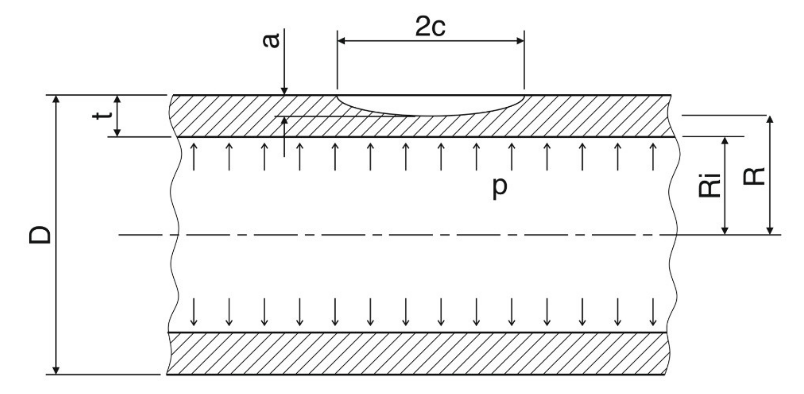
In principle, we proceeded in the same way as we did in Chapter 3 for CCP, DECP, and SECP specimens. This means that we firstly determined the limit load parameter C, and then modified the basic equations of the FC and GSM methods for a thin-walled cylindrical shell with a longitudinal semi-elliptical part-through crack as illustrated in Figure 19.
To be consistent with the form of the J integral, relations for the CCP, DECP, and SECP panels, we started with Equation (20). Considering , where P is the load-per-unit length acting on the pipe wall in the circumferential direction due to pressure p, and PL is the limit load due to the limit pressure pL, Equation (20) obtains the form:
Equation (39) is considered satisfactory for 0.1 < a/(2c) < 0.5 and a/t ≤ 0.8. For a/(2c) < 0.1 the parameter η is equal to (1 − a/t). The yield pressure pY can be determined by inserting σn = σ0 into (38), and expressing σφ as pY R/t. We then obtained:
There are several formulae for the determination of the limit pressure pL for a longitudinal semi-elliptical part-through crack in a thin-walled pipe. We can use the Formula (41) which is published in [23]
where
The symbol σfs in (41) stands for the flow stress, taken as 1.1 times the yield stress σ0. The symbol Ri in (41) and (42) stands for the internal radius, as illustrated in Figure 19. As stated in [23], Equations (41) and (42) give a lower bound estimate of the global collapse pressure. Owing to this, fracture pressures predicted by the GSM and FC methods will be more conservative.
After substituting pL in (37) by (41) and pY in (37) by (40), and considering σfs = 1.1 × σ0 we arrived at (43):
It can be seen from this equation that the limit load parameter C depended on (i) the ratio of the mean radius to the internal radius, and (ii) the geometrical parameters of the pipe and the crack. In the next step we determined the stress intensity factor K for the configuration displayed in Figure 19. We started with the stress intensity factor for a semi-elliptical part-through crack in a sheet. It was found that, for this case, a good engineering assessment of the stress intensity factor was provided by Newman [28]. A modified form of his solution for a longitudinal semi-elliptical part-through crack in a thin-walled pipe is expressed by the relation (44)
where MF is a function dependent on the geometry of a crack (ratio a/c), is an elliptical integral of the second kind, s is a function dependent on the geometry of a crack (ratio a/c) and on its relative depth a/t and, is the correction factor for the curvature of the cylindrical shell and for an increase in stress owing to radial strains in the vicinity of the crack tip.
In the last relationship, MT is the Folias correction factor determined by the relation (45):
In order to compare the conservatism of J predictions made by the GSM and FC methods, we used the two methods to construct J–p dependences for longitudinal part-through cracks with the surface half-length c = 5 t and the relative depth a/t = 1/3, 1/2, and 3/4 in the X70 steel pipe segment. To do so we first modified Equations (21), (30) and (31) to obtain
where ξ is given by the relation (42).
The J–p dependences, determined by Equations (46)–(48), are presented in Figure 20 for the X70 steel pipe segment. The parameters α, n, σfs, as used in Equations (46)–(48), are those given in Table 3.
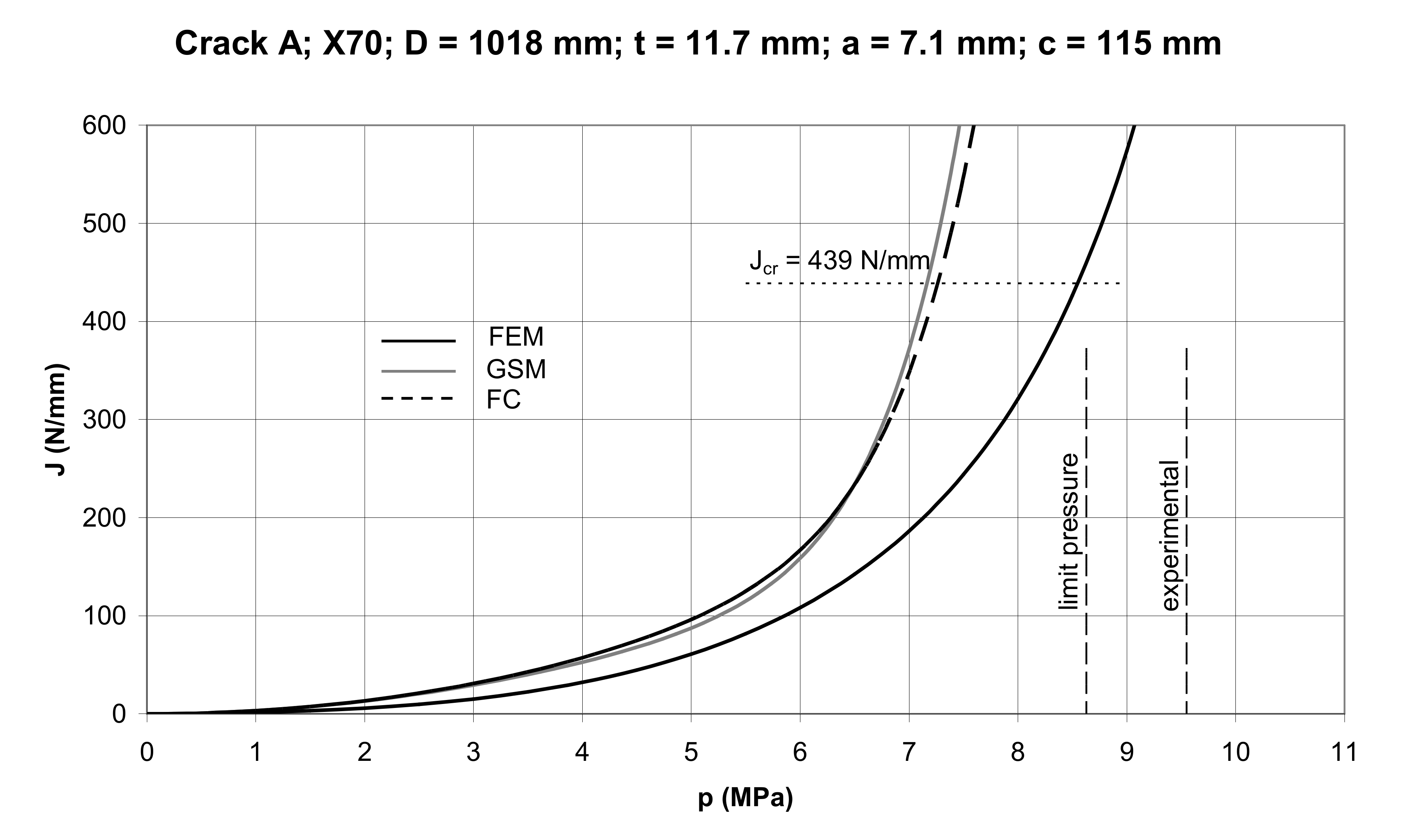
As can be seen in Figure 20, the GSM method is more conservative than the FC method; the difference in the conservatism of the J prediction decreasing with the crack depth. It becomes practically negligible for the relative crack depth a/t = 3/4. By substituting concrete sizes for crack A and B into Equations (46)–(48) we can construct J–p dependences for these cracks using the GSM and FC methods as illustrated in Figure 21 and Figure 22. These curves are compared to the FEM curves computed using the ABAQUS software (ABAQUS Deutschland GmbH, München, Germany). The quarter pipe model with a longitudinal external crack was created. The pipe was loaded by internal pressure and corresponding axial stress. The magnitudes of the internal pressure ranged from 0–9 MPa with a step of 0.5 MPa. The FE-based commercial software ABAQUS was used for the evaluation of the J integral around the crack front in the plane of symmetry. In the region of interest, the elements with full integration and hybrid formulation were used. The characteristic element length at the vicinity of the crack was about 0.05mm.
It is seen here that the fracture pressure is determined as an x co-ordinate of the point of intersection of the appropriate curve with the horizontal Jcr. The limit pressure given by Equation (41) with Equation (42), and the fracture pressure determined experimentally, are also represented here.
Data regarding the geometry of the pipe, the sizes of cracks at fracture, as well as the actual fracture pressures, are summarized in Table 4. The results of determining the fracture pressures using the GSM, FC, and FE methods (pGS, pFC, pFE) from the diagrams in Figure 21 and Figure 22, limit pressures pL determined by Equation (41), and experimental pressures pf, are presented in Table 5.
5. Discussion of Results
5.1. Cracked Panels
Before evaluating and discussing the J integral predictions made using the FC and GSM methods, it should be noted that the resulting J–σ curves were compared to the “reference” J–σ curves determined by the EPRI method. With some exceptions, the EPRI curves can be considered to be sufficiently accurate. If we considered other published methods or procedures for the J integral assessment, it may be found that they are mostly concerned with concrete structural components subjected to specific loads with a partial employment of FEM calculation [29,30]. Finally, the EPRI method appeared to be highly qualified to provide sufficiently accurate J integral predictions. Moreover, the FC method (RCC-MRx Code) to which the GSM method is compared, is generally recognized as a standard used in the design of research reactors.
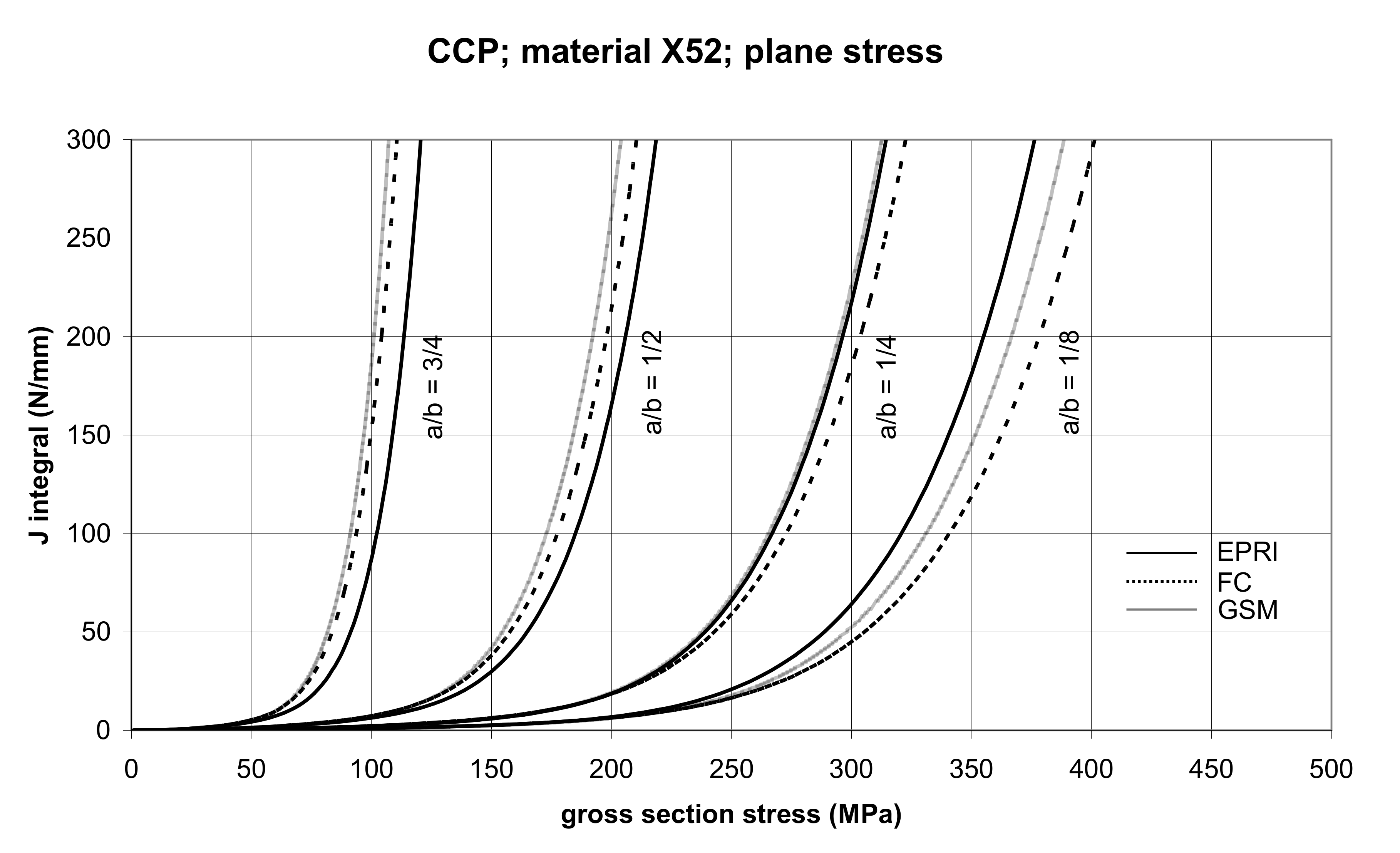
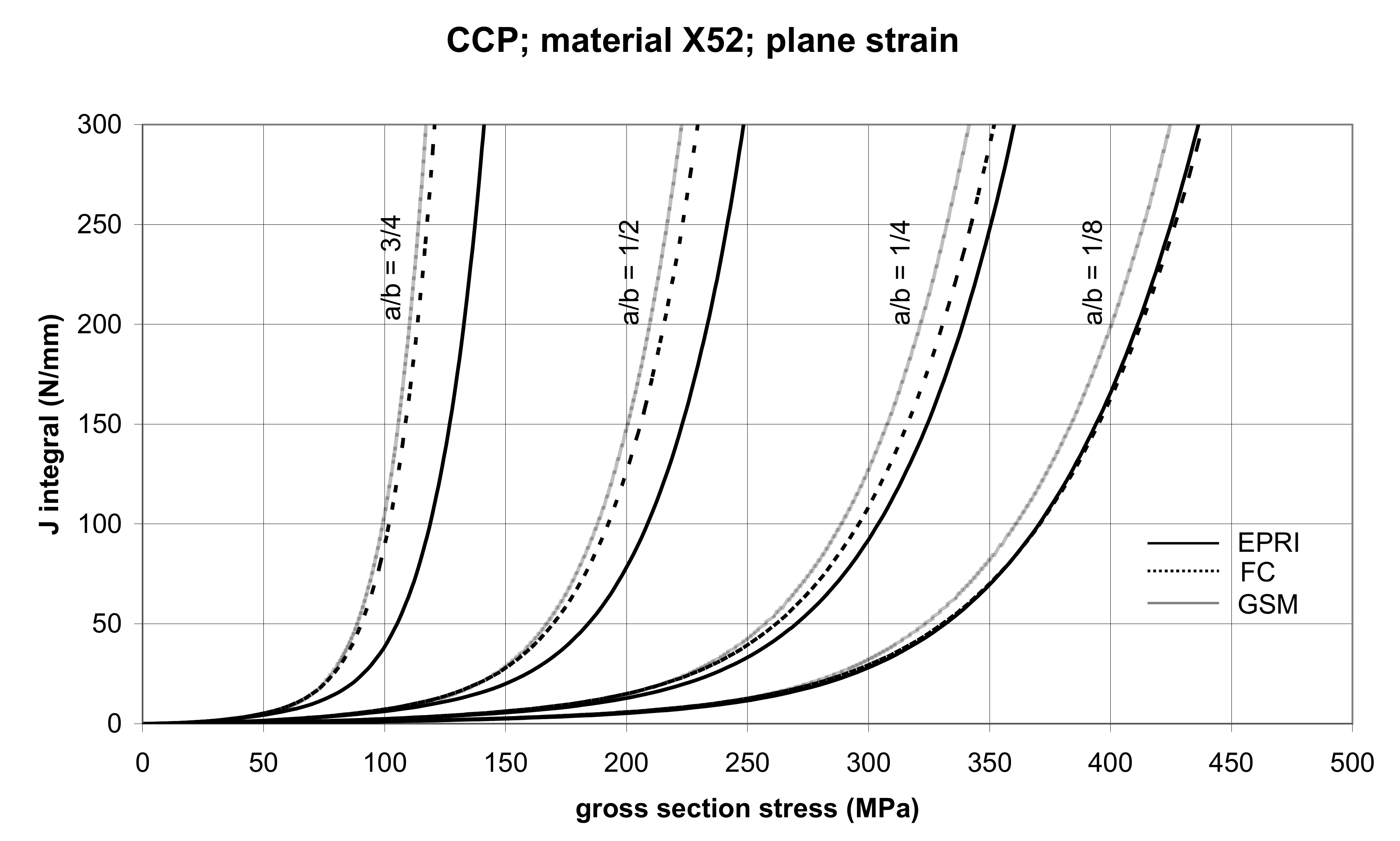
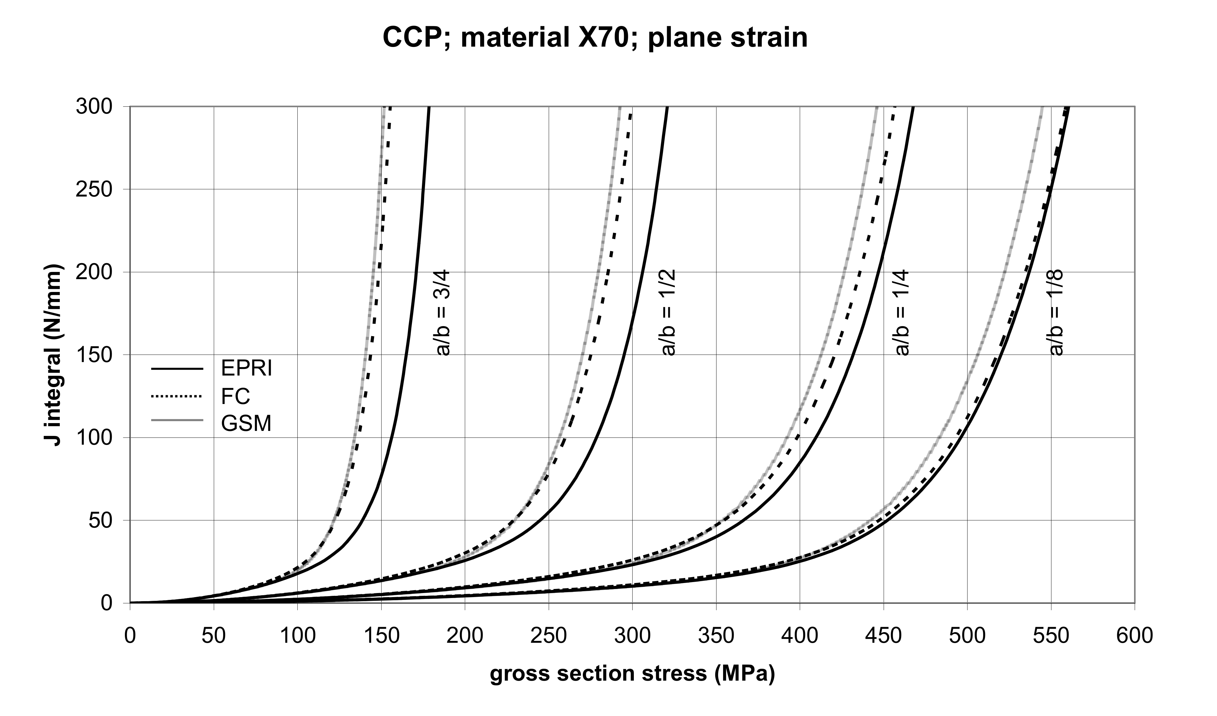
In principle, we can compare the FC and GSM J–σ curves among themselves, and then we can compare them with the EPRI J–σ curves. As seen in Figure 6, Figure 7, Figure 8, Figure 9, Figure 10, Figure 11, Figure 12, Figure 13, Figure 14, Figure 15, Figure 16 and Figure 17, the predicted FC and GSM curves beyond the SSY region are very steep, despite being relatively close to each other with the maximum differences in J values being around 20%. However, from a practical viewpoint, it is more advantageous to compare the FC and GSM curves on the basis of critical (fracture) gross section stress. For the highest value of the J integral in Figure 6, Figure 7, Figure 8, Figure 9, Figure 10, Figure 11, Figure 12, Figure 13, Figure 14, Figure 15, Figure 16 and Figure 17 (300 N/mm), the differences in gross section stresses as determined by the FC and GSM methods were 10–14 MPa for the relative crack length a/b = 1/8; 5–12 MPa for the relative crack length a/b = 1/4; 1–7 MPa for a/b = 1/2 and 1–5 MPa for a/b = 3/4. When we referred these differences to the corresponding gross section stresses, we found that the relative stress differences vary between 0.8% and 3.5%. From the diagrams presented in Figure 6, Figure 7, Figure 8, Figure 9, Figure 10, Figure 11, Figure 12, Figure 13, Figure 14, Figure 15, Figure 16 and Figure 17, it follows that FC and GSM predictions of J integral for specimens CCP, DECP and SECP were conservative for most of the configurations. The situations, when they are not conservative, are connected with small crack lengths (a/b = 1/8). The FC prediction is also not conservative for (i) X52 and X70 CCP plane stress specimens of a/b = 1/4, and (ii) X52 and X70 DECP plane stress specimens of a/b = 1/4. The GSM predictions were slightly more conservative than the FC predictions for all the cases investigated, with one exception being the X52 DECP plane stress specimens of a/b = 1/8. The biggest differences between the J integral predictions made using the FC and GSM methods, on the one hand, and those made using the EPRI method, on the other hand, were found to be for small cracks (a/b = 1/8) in both the X52 and X70 DECP specimens in plane stress as well as in most configurations of SECP specimens from both steels.
5.2. Cracked Pipes
As seen from the data in Table 5, the predicted magnitudes of the fracture pressure were conservative for both cracks. Those obtained by the GSM and FC method were close to each other, although the GSM predictions were slightly more conservative. The FEM prediction, although supposed to provide accurate results, appeared to predict conservative fracture pressures. The likely reason for this was the substitution of the real stress–strain dependence of steel with the Ramberg–Osgood approximation. When plotting these two curves on one diagram it could be seen that, from a certain point on the σ–ε curve onward, the Ramberg–Osgood stress became steadily greater than the actual stress, resulting in a greater strain energy density and thus in a higher magnitude of the J integral. The predicted fracture pressure for J = Jcr then became naturally smaller than that found experimentally. As a matter of interest, Figure 21 and Figure 22 showed that the FEM predicted fracture pressures came close to the limit load pressures determined by Equation (41).
6. Conclusions
The main objective of this study was (i) to compare the J integral assessments as performed by the GSM and FC methods for the center-cracked panels (CCP), double-edge cracked panels (DECP), and single-edge cracked panels (SECP) made from steels X52 and X70, with predictions by the EPRI method, and (ii) to compare the J integral assessments as performed by the GSM and FC methods for a longitudinally cracked pipe produced from X70 steel, with the results obtained by finite element calculations and with the resulting burst pressures obtained experimentally. Both aspects of the main objective were achieved.
The results of J integral predictions for cracked panels showed that both methods provided very close predictions. In comparison with the EPRI results, these predictions were found to be conservative in most cases. The GSM predictions are slightly more conservative than the FC predictions for all the cases investigated, with one exception referring to X52 DECP plane stress specimens of a/b = 1/8.
The J integral predictions by the FC and GSM methods for the longitudinally cracked pipe appeared to be very close, the GSM prediction being slightly more conservative than the FC prediction. However, these predictions were widely conservative in comparison with the prediction by the FEM analysis. As far as the fracture toughness Jcr = 439 N/mm for X70 steel is concerned, the corresponding magnitudes of the burst pressure for two longitudinal part-through cracks were: 7.16–7.38 MPa according to GSM and FC; 8.56–8.60 MPa according to FEM; and 9.55–9.86 MPa obtained experimentally. It follows from this that there exists a high degree of conservatism in predicting burst pressures of cracked pipes on the basis of the GSM and FC methods.
However, when operating high-pressure pipelines or cylindrical pressure vessels, the most important aspects that should be observed are the safety of the operation and the integrity of the pressure systems throughout their entire projected lifetime. It is for this reason that such methods of assessment of the life of pressure vessels and pipelines are preferred; so that they provide a conservative prediction of burst pressure across a wide range of possible stress states. With regard to thin-walled cylindrical pressure vessels and pipelines, the FC and GSM methods can be ranked among such methods. It has been proven here that the predictions of the J integral for thin-wall pressure pipelines using the FC and GSM methods is more conservative than those made using the FE method. On the other hand, the FE method provided lower magnitudes of fracture pressure than those found experimentally, i.e., it was conservative. It is very likely that the cause for this disagreement consists in substituting the real stress–strain dependence of the steel with the Ramberg–Osgood approximation.
Finally, it can be stated that the main contribution of this study is verification of the applicability of the newly developed GSM method for assessment of the J integral for cracked plates and pipes. Together with the FC method, it can be used for a conservative prediction of fracture parameters for cracked plates as well as for cylindrical pressure vessels and pipelines with relatively deep longitudinal part-through cracks.
Author Contributions
Conceptualization, Ľ.G.; methodology, Ľ.G. and M.Š.; software, J.K. and J.B.; validation, Ľ.G. and M.Š.; formal analysis, Ľ.G.; funding acquisition, M.Š.; investigation, Ľ.G.; project administration, Ľ.G. and M.Š.; resources, Ľ.G. and M.Š.; supervision, Ľ.G. and M.Š.; visualization, Ľ.G. and M.Š.; writing—original draft, Ľ.G.; writing—review and editing, Ľ.G. and M.Š. All authors have read and agreed to the published version of the manuscript.
Funding
This research was funded by the Technological Agency of the Czech Republic, grant number FW 01010021.
Institutional Review Board Statement
Not applicable.
Informed Consent Statement
Not applicable.
Data Availability Statement
All data generated or analyzed during this study are included in this published article.
Acknowledgments
The authors gratefully appreciate the help of CEPS Company in realization of hydraulic tests of a cracked pipe segment.
Conflicts of Interest
The authors declare no conflict of interest.
Notation
The following symbols are used in this paper:
| a | = crack length (depth); |
| b | = specimen width; |
| c | = half crack length; |
| C | = limit load parameter; |
| D | = outside diameter of a pipe; |
| E | = Young’s modulus; |
| f | = specific function of the ratio a/b for cracked specimens; |
| J, Jcr | = J integral, critical J integral; |
| Je | = elastic component of J integral; |
| Jm | = J integral corresponding to the maximum load in testing CT specimens; |
| Jpl | = plastic component of J integral; |
| kt | = theoretical stress concentration factor; |
| KI, KI p | = stress intensity factor for mode I, provisional KI; |
| n | = Ramberg–Osgood exponent; |
| p | = internal pressure in a pipe; |
| pL | = limit internal pressure; |
| pY | = yield internal pressure; |
| P | = acting load; |
| P0 | = reference load; |
| PL | = limit load; |
| R, Ri | = mean radius, internal radius of a pipe; |
| Rm | = ultimate tensile strength; |
| t | = wall thickness of a pipe; |
| w | = strain energy density; |
| α | = Ramberg–Osgood constant; |
| εo | = elastic strain at the yield stress; |
| εe | = elastic strain at the reference stress; |
| εref | = reference strain; |
| η, ξ | = geometric parameters for a surface semi-elliptical crack in a pipe wall; |
| σn | = net section stress or hoop stress in the ligament surrounding a longitudinal surface crack in a pipe wall; |
| σo | = yield stress; |
| σref | = reference stress; |
| σfs | = flow stress; |
| σφ | = hoop stress; |
| (ρ, θ) | = polar coordinates of a point on the periphery of the notch root; |
| φ | = correction function for small plastic zone; |
| ψ | = geometric parameter for SECP specimens; |
References
- Gajdoš, Ľ.; Srnec, M. An approximate method for J integral determination. Acta Tech. CSAV 1994, 39, 151–171. [Google Scholar]
- RCC-MR. Design and Construction Rules for Mechanical Components of FBR Nuclear Island, 1st ed.; French Association for the Design, Construction and Operating Supervision of the Equipment for Electronuclear Boilers (AFCEN): Paris, France, 1985; Volume 18. [Google Scholar]
- Rice, J.R. A path independent integral and the approximate analysis of strain concentration by notches and cracks. J. Appl. Mech. 1968, 35, 379–386. [Google Scholar] [CrossRef] [Green Version]
- Funari, M.F.; Lonetti, P.; Spadea, S. A crack growth strategy based on moving mesh method and fracture mechanics. Theor. Appl. Fract. Mech. 2019, 102, 103–115. [Google Scholar] [CrossRef]
- Tankasala, H.C.; Li, T.; Seiler, P.E.; Deshpande, V.S.; Fleck, N.A. An assessment of the J-integral test for a metallic foam. J. Mech. Phys. Solids 2020, 141, 103958. [Google Scholar] [CrossRef]
- Zhang, Z.; Yang, F.; Liu, Y.; Wang, L. J-integral evaluation of a mode I crack in gradient nanocrystalline metals. Mater. Today Comm. 2020, 25, 101328. [Google Scholar] [CrossRef]
- Tada, H.; Paris, P.C.; Irwin, R. The Stress Analysis of Cracks Handbook; Del Research Corporation: Hellertown, PA, USA, 1973. [Google Scholar]
- Rooke, D.P.; Cartwright, D.J. Compendium of Stress Intensity Factors; Her Majesty’s Stationery Office: London, UK, 1974. [Google Scholar]
- Murakami, Y. Stress Intensity Factors Handbook; The Society of Materials Science, Pergamon Press: Tokyo, Japan, 1987. [Google Scholar]
- Marie, S.; Chapuliot, S.; Kayser, Y.; Lacire, M.H.; Drubay, B.; Barthelet, B.; Triay, M. French RSE-M and RCC-MR code appendices for flaw analysis. Presentation of the fracture parameters calculation- Part I, General overview. Int. J. Pres. Ves. Pip. 2007, 84, 590–600. [Google Scholar] [CrossRef]
- Muñoz Garcia, J.E.; Petesch, C.; Lebarbé, T.; Bonne, D.; Gelineau, O.; Pascal, C.; Blat, M. Design and construction rules for mechanical components of high-temperature, experimental and fusion nuclear installations. The RCC-MRx Code last edition. Bull. JSME Mech. Eng. J. 2020, 7, 1–12. [Google Scholar]
- Ainsworth, R.A. The assessment of defects in structures of strain hardening material. Eng. Fract. Mech. 1984, 9, 633–642. [Google Scholar] [CrossRef]
- Matvienko, Y.G.; Morozov, E.M. Inter-relationship of non-linear fracture mechanics criteria. Phys. Chem. Mech. Mater. 1989, 25, 3–10. (In Russian) [Google Scholar]
- Matvienko, Y.G.; Morozov, E.M. Calculation of the energy J-integral for bodies with notches and cracks. Int. J. Fract. 2004, 125, 249–261. [Google Scholar] [CrossRef]
- Matvienko, Y.G. J-estimation formulas for non-linear crack problems. Int. J. Fract. 1994, 68, R15–R18. [Google Scholar] [CrossRef]
- Norio, H.; Yasuhiro, K. Calculation of stress intensity factor from stress concentration factor. Eng. Fract. Mech. 1978, 10, 215–221. [Google Scholar] [CrossRef]
- Glinka, G. Energy density approach to calculation of inelastic strain- stress near notches and cracks. Eng. Fract. Mech. 1985, 22, 485–508. [Google Scholar] [CrossRef]
- Kumar, V.; German, M.D.; Shih, C.F. An engineering approach for elastic- plastic fracture analysis. In Prepared for Electric Power Research Institute (EPRI); General Electric Co.: Schenectady, NY, USA, 1981. [Google Scholar]
- Milne, I.; Ainsworth, R.A.; Dowling, A.R.; Stewart, A.T. Assessment of the integrity of structures containing defects. Int. J. Press. Vessel. Pip. 1988, 32, 3–104. [Google Scholar] [CrossRef]
- Gajdoš, Ľ.; Šperl, M. Application of a fracture-mechanics approach to gas pipelines. Int. J. Mech. Mechatron. Eng. 2011, 5, 67–74. [Google Scholar]
- Gajdoš, Ľ.; Šperl, M. Evaluating the integrity of pressure pipelines by fracture mechanics. In Applied Fracture Mechanics; Belov, A., Ed.; InTech: Rijeka, Croatia, 2012; pp. 283–310. [Google Scholar]
- Gajdoš, Ľ.; Šperl, M. Critical conditions of pressurized pipes. Eng. Mech. 2013, 20, 401–412. [Google Scholar]
- Miller, A.G. Review of limit loads of structures containing defects. Int. J. Pres. Ves. Pip. 1988, 32, 197–327. [Google Scholar] [CrossRef]
- Anderson, T.L. Fracture Mechanics, Fundamentals and Applications. Part V: Reference Material–Compilation of K, J, Compliance and Limit Load Solutions, 2nd ed.; CRC Press: Boca Raton, IL, USA, 1995; pp. 601–654. [Google Scholar]
- Witek, M. Structural integrity of steel pipeline with clusters of corrosion defects. Materials 2021, 14, 852. [Google Scholar] [CrossRef] [PubMed]
- Nykyforchyn, H.; Zvirko, O.; Dzioba, I.; Krechkovska, H.; Hredil, M.; Tsyrulnyk, O.; Student, O.; Lipiec, S. Assessment of operational degradation of pipeline steels. Materials 2021, 14, 3247. [Google Scholar] [CrossRef]
- Harrison, R.P.; Loosemore, K.; Milne, I.; Dowling, A.R. Assessment of the Integrity of Structures Containing Defects; CEGB Report R/H/R6–Rev. 2; Central Electricity Generating Board, Research Division: London, UK, 1980. [Google Scholar]
- Newman, J.C. Fracture analysis of surface and through-cracked sheets and plates. Eng. Fract. Mech. 1973, 5, 667–689. [Google Scholar] [CrossRef]
- Rahman, S.; Brust, F.W. Approximate methods for predicting J- integral of a circumferentially surface-cracked pipe subject to bending. Int. J. Fract. 1997, 85, 111–130. [Google Scholar] [CrossRef]
- Sharma, R.K.; Shrivastava, S.K.; Dixit, P.M.; Basu, S. On the problem of an axial semi-elliptical crack in a hollow ductile cylinder. Int. J. Fract. 2006, 140, 269–275. [Google Scholar] [CrossRef]
Figure 1.
A section of a notched body, loaded by a remote uniform stress, and an indication of the path of integration.
Figure 1.
A section of a notched body, loaded by a remote uniform stress, and an indication of the path of integration.

Figure 2.
Polar co-ordinates of a point on the semicircular periphery of the notch.

Figure 3.
Ramberg–Osgood stress–strain diagram and denotation of the quantities used.

Figure 4.
Specimens used in the investigations.

Figure 5.
The stress-strain curves for the steels used.

Figure 6.
Comparison of J integral for CCP X52 steel specimens in the plane stress condition as determined by the EPRI, GSM, and FC methods.
Figure 6.
Comparison of J integral for CCP X52 steel specimens in the plane stress condition as determined by the EPRI, GSM, and FC methods.

Figure 7.
Comparison of J integral for CCP X52 steel specimens in the plane strain condition as determined by the EPRI, GSM, and FC methods.
Figure 7.
Comparison of J integral for CCP X52 steel specimens in the plane strain condition as determined by the EPRI, GSM, and FC methods.

Figure 8.
Comparison of J integral for CCP X70 steel specimens in the plane stress condition as determined by the EPRI, GSM, and FC methods.
Figure 8.
Comparison of J integral for CCP X70 steel specimens in the plane stress condition as determined by the EPRI, GSM, and FC methods.

Figure 9.
Comparison of J integral for CCP X70 steel specimens in the plane strain condition as determined by the EPRI, GSM, and FC methods.
Figure 9.
Comparison of J integral for CCP X70 steel specimens in the plane strain condition as determined by the EPRI, GSM, and FC methods.

Figure 10.
Comparison of J integral for DECP X52 steel specimens in the plane stress condition as determined by the EPRI, GSM, and FC methods.
Figure 10.
Comparison of J integral for DECP X52 steel specimens in the plane stress condition as determined by the EPRI, GSM, and FC methods.

Figure 11.
Comparison of J integral for DECP X52 steel specimens in the plane strain condition as determined by the EPRI, GSM, and FC methods.
Figure 11.
Comparison of J integral for DECP X52 steel specimens in the plane strain condition as determined by the EPRI, GSM, and FC methods.

Figure 12.
Comparison of J integral for DECP X70 steel specimens in the plane stress condition as determined by the EPRI, GSM, and FC methods.
Figure 12.
Comparison of J integral for DECP X70 steel specimens in the plane stress condition as determined by the EPRI, GSM, and FC methods.

Figure 13.
Comparison of J integral for DECP X70 steel specimens in the plane strain condition as determined by the EPRI, GSM, and FC methods.
Figure 13.
Comparison of J integral for DECP X70 steel specimens in the plane strain condition as determined by the EPRI, GSM, and FC methods.

Figure 14.
Comparison of J integral for SECP X52 steel specimens in the plane stress condition as determined by the EPRI, GSM, and FC method.
Figure 14.
Comparison of J integral for SECP X52 steel specimens in the plane stress condition as determined by the EPRI, GSM, and FC method.

Figure 15.
Comparison of J integral for SECP X52 steel specimens in the plane strain condition as determined by the EPRI, GSM, and FC methods.
Figure 15.
Comparison of J integral for SECP X52 steel specimens in the plane strain condition as determined by the EPRI, GSM, and FC methods.

Figure 16.
Comparison of J integral for SECP X70 steel specimens in the plane stress condition as determined by the EPRI, GSM, and FC methods.
Figure 16.
Comparison of J integral for SECP X70 steel specimens in the plane stress condition as determined by the EPRI, GSM, and FC methods.

Figure 17.
Comparison of J integral for SECP X70 steel specimens in the plane strain condition as determined by the EPRI, GSM, and FC methods.
Figure 17.
Comparison of J integral for SECP X70 steel specimens in the plane strain condition as determined by the EPRI, GSM, and FC methods.

Figure 18.
A view of testing pipes in the working pit.

Figure 19.
A longitudinal semi-elliptical part-through crack in a thin-walled pipe.

Figure 20.
The J–p dependences for the X70 steel pipe segment with part-through cracks of various relative depths and of relative surface length 2c/t = 10.
Figure 20.
The J–p dependences for the X70 steel pipe segment with part-through cracks of various relative depths and of relative surface length 2c/t = 10.

Figure 21.
J–p dependences for Crack A.

Figure 22.
J–p dependences for Crack B.


Table 1.
The Ramberg–Osgood parameters and ultimate strengths of the steels used.
| Material | Characteristics | |||
|---|---|---|---|---|
| α (1) | n (1) | σ0 (MPa) | Rm (MPa) | |
| X52 | 2.40 | 6.25 | 313 | 493 |
| X70 | 5.92 | 9.62 | 536 | 644 |
Table 2.
Limit load parameters for the specimens used.
| Specimen | C | |
|---|---|---|
| Plane Stress | Plane Strain | |
| CCP | 1 | 2/√3 |
| DECP | 2/√3 | 0.91 + 0.36/(1 − a/b) |
| SECP | 1.072 ψ | 1.455 ψ |
A note: parameter ψ is given by Equation (32).
Table 3.
Some characteristics referring to the pipe segment.
| Characteristics | Crack A | Crack B |
|---|---|---|
| Crack dimensions | ||
| half-length, c (mm) | 115 | 127 |
| depth in fracture, af (mm) | 7.1 | 6.7 |
| Ramberg–Osgood parameters | ||
| α/n/σ0 (MPa) | 5.92/9.62/536 | 5.92/9.62/536 |
| Flow stress | ||
| σfs (MPa) | 590 | 590 |
| Fracture toughness | ||
| Jcr = Jm (N/mm) | 439 | 439 |
| Fracture pressure | ||
| pf (MPa) | 9.55 | 9.86 |
Table 4.
Geometric characteristics of the pipes with cracks, crack depth at fracture, and fracture pressure.
Table 4.
Geometric characteristics of the pipes with cracks, crack depth at fracture, and fracture pressure.
| Quantity | Ri (mm) | t (mm) | c (mm) | af (mm) | pf (MPa) |
|---|---|---|---|---|---|
| Crack A | 497.8 | 11.7 | 115 | 7.1 | 9.55 |
| Crack B | 497.8 | 11.7 | 127 | 6.7 | 9.86 |
Table 5.
Comparison of predicted and experimental fracture pressures.
| Quantity | pGS (MPa) | pFC (MPa) | pFEM (MPa) | pL (MPa) | pexp = pf (MPa) |
|---|---|---|---|---|---|
| Crack A | 7.16 | 7.26 | 8.56 | 8.63 | 9.55 |
| Crack B | 7.26 | 7.38 | 8.60 | 8.61 | 9.86 |
Publisher’s Note: MDPI stays neutral with regard to jurisdictional claims in published maps and institutional affiliations. |
© 2021 by the authors. Licensee MDPI, Basel, Switzerland. This article is an open access article distributed under the terms and conditions of the Creative Commons Attribution (CC BY) license (https://creativecommons.org/licenses/by/4.0/).
Share and Cite
MDPI and ACS Style
Gajdoš, Ľ.; Šperl, M.; Bayer, J.; Kuželka, J. Comparison of J Integral Assessments for Cracked Plates and Pipes. Materials 2021, 14, 4324. https://doi.org/10.3390/ma14154324
AMA Style
Gajdoš Ľ, Šperl M, Bayer J, Kuželka J. Comparison of J Integral Assessments for Cracked Plates and Pipes. Materials. 2021; 14(15):4324. https://doi.org/10.3390/ma14154324
Chicago/Turabian StyleGajdoš, Ľubomír, Martin Šperl, Jan Bayer, and Jiří Kuželka. 2021. "Comparison of J Integral Assessments for Cracked Plates and Pipes" Materials 14, no. 15: 4324. https://doi.org/10.3390/ma14154324
Note that from the first issue of 2016, this journal uses article numbers instead of page numbers. See further details here.