

Abstract
We have recently designed a new type of a flat metal-dielectric grating which is supposed to replace blazed diffraction gratings, providing very high −1st reflected diffraction order efficiency within a broad wavelength band, high durability, and relative ease of fabrication. In this communication we present a rigorous electromagnetic theory of the grating in the approximation of infinitely thin perfect metal and show that the properly designed grating can reach 100% diffraction efficiency in the Littrow configuration for either transversal electric (TE or s) or transversal magnetic (TM or p) polarizations. Properties of the grating are analysed and discussed in detail.
Export citation and abstract BibTeX RIS

Original content from this work may be used under the terms of the Creative Commons Attribution 4.0 license. Any further distribution of this work must maintain attribution to the author(s) and the title of the work, journal citation and DOI.
1. Introduction
Nanophotonic devices operating under leaky-mode resonance conditions have attracted considerable interest over the years. Flexibility in their design allows to achieve extremely narrowband resonances in weakly corrugated structures [1] or very broadband operation in strongly modulated resonant gratings [2–4]. In theory, these devices allow to achieve 100% diffraction efficiency [5], and more than 99% has been reported in experiments [6]. They are based on the leaky-mode resonance, which was recognized in some of Wood's diffraction anomalies by Hessel and Oliner [7] and further theoretically studied in dielectric gratings combined with waveguides by Neviere et al [8]. Numerous applications of leaky-mode resonance gratings include polarizers [9], mirrors in vertical cavity surface emitting laser (VCSEL) diodes [10], enhancement of mid-infrared absorption in solar cells [11, 12], biosensors [13, 14], etc.
The grating described here has the form of a metallic parallel-plate waveguide with periodic slits in one metal sheet. However, since we do not primarily consider the normal incidence but the Littrow configuration, the waveguide analysis is not appropriate. Moreover, in this case, the 'waveguide' is so strongly leaky that no perturbation analysis can be applied. Instead, we present a rigorous electromagnetic analysis of the grating behaviour based on the Rayleigh expansion [15]. The parallel plates are approximated with infinitely thin 'perfect metal' sheets. Usually, a 'perfect metal' is considered as a material with infinitely large electric conductivity, which leads to the requirement of zero tangential component of electric field intensity at its surface. However, metals in the optical spectral domain behave rather differently; some of them—especially mostly used metals like Ag, Au and Al—exhibit strongly negative real parts and relatively small imaginary parts of their relative permittivities. It is easy to show that the approximation of an infinitely large negative real part of the permittivity leads to the same boundary condition as for a perfect metal—zero tangential component of the electric field intensity at the surface. The electromagnetic field in the medium with the (real) relative permittivity  is damped because of the imaginary propagation constant
  . For
. For  , the electromagnetic field inside the medium must vanish, similarly as the field inside the perfect conductor. Because of this, the boundary conditions for a perfectly conducting metal and 'perfect optical metal' have to be identical. We will thus use this boundary condition in our further considerations. Numerical simulation of the grating with realistic parameters of the metal layer, successful experimental demonstration of the grating performance, and its practical implementation as a mirror of a tuneable laser have already been presented in our recent paper [16]. The diffraction efficiency into the −1st reflected order in Littrow configuration, measured on a fabricated grating, was higher than 90% in the spectral range of 1417–1700 nm.
2. Theory
The cross-section of the grating considered here is shown in figure 1.
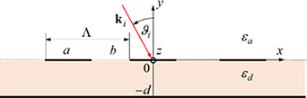
Figure 1. Cross-section of the idealized diffraction grating.
Download figure:
Standard image High-resolution imageIt consists of a lossless dielectric layer of the thickness d and a relative permittivity  , both sides of which are covered with layers of a 'perfect metal'. The bottom metal layer is uniform, the upper layer has the form of periodic stripes of the width a, separated by the slits of the width b. The period of the grating is thus
  (figure 1). The metal stripes are considered unlimited in the
  direction, and their thickness is assumed infinitesimally small. The grating is illuminated with a plane wave with the wave vector
  impinging under the incidence angle
  within the plane
  , i.e. perpendicular to the stripes. Here,
  is the free-space wavenumber,
 and
and  are the unit vectors of the coordinate system
  . Under such conditions, all quantities (both the permittivity and electromagnetic field distributions) are independent of the z-coordinate,
  which makes the problem two-dimensional, and it allows to consider the cases of transversal electrical (TE) (s) and transversal magnetic (TM) (p) polarizations separately.
2.1. TM polarization
Let us start with the analysis of the TM polarization. In this case, the magnetic field intensity has the only component  while the electric field intensity has two components,
  The electromagnetic field vectors of the incident plane wave are
where  is the free-space impedance. The complex representation of the time harmonic dependence of the form
  is supposed and suppressed. The layered structure of the grating allows us to calculate the distributions of tangential field components
  only; the vertical field component
  can then be easily found from Maxwell equations. Due to the periodicity of the grating structure, the field distribution of the reflected wave in the region
  above the grating is given by the superposition of plane waves—diffraction orders of the grating:
The field within the dielectric layer between the metal layers is composed of plane waves propagating upwards and downwards with respect to the coordinate axis y:
In the last equation in (3), all upper or all lower signs are to be taken simultaneously. At the bottom interface with the metal,  the tangential component of the electric field intensity,
  must be equal to zero for any x. From (3) it immediately follows that

The tangential field components just below the metal stripes at  can then be expressed by using of only one set of amplitudes:
At this interface, the boundary conditions are more complicated. At the metalized sections, the tangential components of the electric field intensity must vanish both above and below the interface:
Within the openings between the metal stripes, the tangential components of both electric and magnetic fields must be continuous:
In order to cope with these complicated boundary conditions, we introduce a periodic rectangular function 
the graph of which is shown in figure 2.

Figure 2. Graph of the rectangular periodic function  .
.
Download figure:
Standard image High-resolution imageThen, the boundary conditions at the metalized parts can be rewritten in the following way:
As long as the conditions (9) are satisfied, we can avoid the specification of the region of validity of the continuity condition (7) for the electric field since outside the openings, the tangential components of the electric field vanish. Thus, we can write the continuity conditions (7) in the form
which is now valid for any x. In view of the first equation in (10), it is sufficient to satisfy just one of the equation (9). However, it means that we still have three equations for two unknown fields  . Inspired with [17], we reduce the number of equations by introducing a dimensionless parameter g and joining two of the three equations into one. We obtain
where  is the vacuum admittance. The value of g is rather arbitrary; the number close to one is a good choice.
Equations (11) can be expressed with the help of the complex amplitudes  only as follows:
Here, we used the substitution  where
where  is the grating constant, and the exponential
  (occurring in all terms) was omitted. Now we can use the first equation in (12) to exclude the terms
  from the second one. By comparing of the exponential terms
  , we obtain

The substitution for  from (13) into the second equation in (12) results after some further manipulations in the following equation:
In order to solve this equation for  , the periodic functions
  and
and  have to be expanded into Fourier series:
After introducing these expansions into (14) and subsequent comparing the complex harmonic terms we obtain the following infinite set of linear equations for  :
:
For numerical solution the number of harmonics and correspondingly also the number of equations has to be limited to a finite number:  Note that this is the only approximation to the solution of the problem. Having solved equation (16), the amplitudes
  are easily determined from (4) and the amplitudes of the reflected waves
  from (13). The electric field amplitudes can be evaluated from (2) and (3). The most important parameters of the grating are the efficiencies of reflected diffraction orders. Since we consider the grating unlimited in the x-direction, the diffraction efficiency of the mth order is determined as a ratio of the power flow density of the diffracted and incident plane waves in the direction perpendicular to the grating plane, respectively, i.e. as a ratio of y-components of the respective time-averaged Poynting vectors. Taking into account equations (1) and (2), we easily obtain the following expression:
As expected, the diffraction efficiency is nonzero only for propagating diffraction orders for which  are real.
2.2. TE polarization
The analysis for the case of TE polarization is very similar, we thus present here only the important relations. The electric and magnetic fields of the incident wave are
In analogy with (2), the tangential field components of the reflected diffraction orders are expressed as
and the tangential components of the fields in the dielectric layer just below the metallic stripes are
Here, the boundary condition at the bottom metal interface,  giving
  , has already been implemented. The boundary conditions at the upper interface with the periodic array of metal stripes result now in the following equations:
where g is an arbitrary number. By inserting of the expansions (19) and (20) into (21) we obtain after rearrangements of the exponential terms the equation

for  and the set of linear equations for the complex amplitudes
Having solved this set of equations (properly limited to 
 where M is of the order of a few hundreds), we obtain the formula
for the efficiency of the mth diffraction order.
3. Grating properties
3.1. Plane-wave analysis
We are interested in the grating behaviour from the point of view of its intended application as a tuning retroreflecting grating mirror for (fibre) lasers operating at the near infrared wavelength range. The wavelength of the incident wave is thus chosen as 1550 nm. In order to avoid the existence of more than a single (−1st) propagating diffraction order (except the 0th order reflected wave), the grating period is fixed at  In this case, the incidence angle for the Littrow (retroreflection) configuration in air
  is
is ![${\vartheta _i} = \arcsin [\lambda /(2\Lambda )] = {53.83^\circ }.$](https://content.cld.iop.org/journals/2040-8986/23/1/015601/revision4/joptabcd01ieqn53.gif) Silica with the relative permittivity
Silica with the relative permittivity  is chosen as a dielectric layer supporting the metalized surfaces. The diffraction efficiency of the grating depends then on the two remaining parameters—the metal filling factor of the grating,
  and the thickness of the dielectric layer d. The dependence of diffraction efficiencies on these parameters are shown in the plots in figure 3 for both TM and TE polarizations.

Figure 3. Diffraction efficiency of the grating in Littrow configuration in dependence of the dielectric layer thickness d and the metal filling factor  . (a) TM polarization, (b) TE polarization.
Download figure:
Standard image High-resolution imageIt is obvious that the diffraction efficiency can reach values very close to one for both TE and TM polarizations, although for different parameters. This situation is apparently more tolerant to variations of the filling factor than to variations of the thickness of the dielectric layer. Figure 4 shows the graphs of the retro-diffraction efficiencies for TM and TE polarizations for the values of the filling factors possessing somewhat relaxed tolerances of the dielectric layer thickness. For TM polarization, the optimum filling factor  corresponds to the width a of the metal stripes (see figure 1) of 432 nm, while their optimum width for TE polarization, corresponding to
  is only about 43 nm.

Figure 4. Diffraction efficiency of the grating in the Littrow configuration versus the thickness of the dielectric layer d. (a) TM polarization,  (b) TE polarization,
Download figure:
Standard image High-resolution imageThe periodically repeating patterns in dependence of the dielectric layer thickness in the diffraction efficiency plots in figures 3 and 4 are primarily due to the Fabry–Perot type resonances between the metal sheets supported by the −1st and 0th propagating diffraction orders. Except for the first pattern for the TM polarization, which will be discussed separately, the period can be unanimously determined as  It exactly corresponds to the phase increment
  of the −1st and 0th diffraction orders propagating in the dielectric layer with the tangential wave vector components
  in the Littrow configuration. Namely,
 ![${k_y} = {k_0}\sqrt {{\varepsilon _d} - {{\left[ {\lambda /(2\Lambda )} \right]}^2}} ,$](https://content.cld.iop.org/journals/2040-8986/23/1/015601/revision4/joptabcd01ieqn74.gif) and
and  as expected.
According to figure 3(a) for the TM polarization, the 100% retro-diffraction efficiency takes place for a particular value of the filling factor  even for an extremely small thickness
  of the order of a few tens of nanometre. It is thus not surprising that in this case, higher diffraction orders, evanescent in the y-direction (perpendicular to the grating), play an important role in the field distribution, affect the resulting phase of the −1st and the 0th diffraction orders, and thus also the position and shape of the first maximum in figure 4(a).
The field distributions in the vicinity of the grating in the Littrow configuration for the optimum parameters for TM and TE polarizations are shown in figure 5. In figure 5(a) the metal grating is represented by black lines while in figure 5(b) the narrow metal stripes are shown by small white rectangles, to improve their visibility. The interface between the dielectric SiO2 layer and air is marked by a magenta line. In figure 5(a) it is shown the distribution of the absolute value of the magnetic field intensity  for the TM polarization at
  and
and  while figure 5(b) displays the distribution of the absolute value of the electric field intensity
  for the TE polarization at
  and
and  Note that in the case of a 100% retro-diffraction efficiency, the optical field has the character of a pure standing wave; the incident wave is totally diffracted backwards, and no power is propagating along the grating plane.
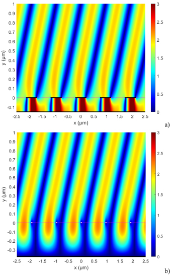
Figure 5. Distribution of field intensities in the vicinity of the grating for  (SiO2). (a) TM polarization, distribution of
  for
for  and
and  (b) TE polarization, distribution of
  for
for  and
and 
Download figure:
Standard image High-resolution imageThe maximum field intensity of the incident wave is normalized to unity, and the total field maxima above the grating are thus twice larger (corresponding to the light orange colour in figure 5). The far-fields for TM and TE polarizations are thus identical, and in both figures, the influence of evanescent waves near the dielectric interface  is apparent. However, there is a marked difference in the field distributions within the dielectric layer. In the case of the TM polarization, the metal stripes and slots have similar widths (which makes its fabrication easier), but there is quite strong accumulation of optical energy within the dielectric layer between the metal layers; the field intensity there is several times stronger than the intensity of the incident wave. On the other hand, it is surprising that in the case of TE polarization, very tiny metal stripes of the width of about
  of the grating period (∼40 nm) lead to 100% retro-diffraction efficiency. There is only very weak field concentration between the metal stripes; however, the fabrication of such a grating is not easy. Let us note for completeness that—in accordance with figure 3(a)—the retro-diffraction efficiency close to 100% can be obtained also for TM polarization with the dielectric layer only 50 nm thick with a filling factor as high as 0.97, i.e. with slits only about 30 nm wide.
3.2. Influence of the permittivity of the dielectric layer
Although the geometry of the grating is very simple, the wave processes leading to such a high diffraction efficiency deserve deeper discussion. Obviously, in order to obtain a 100% retro-diffraction efficiency, the reflected wave (the 0th reflected diffraction order) has to be cancelled out by the destructive interference of all waves propagating in the same direction after (multiple) reflections and diffractions at the metal sheets. (Note that in the far field zone of the grating,  which is utilized for technical applications, only the propagating −1st and 0th reflected diffraction orders are important.)
In order to investigate the role of the permittivity of the dielectric layer  between the metal sheets, we calculated the retro-diffraction efficiency of the grating for the two more cases,
  (air) and
  (silicon). The results are presented in figure 6 for the TM polarization; the results for the TE polarization are fully analogical and for brevity they are not presented.

Figure 6. Diffraction efficiency of the grating in the Littrow configuration in dependence of the dielectric layer thickness d and the metal filling factor  for TM polarization. (a)
  (air) and (b)
  (silicon).
Download figure:
Standard image High-resolution imageThe hypothetic case of  was chosen in order to demonstrate that the existence of the dielectric interface in the slits between metal stripes does not play any important role; in this case it is namely missing. The main effect of the lower permittivity is that, in order to preserve the necessary optical path between the metal layers, the optimum thickness of the layer is increased. On the other hand, the dominant effect of the high permittivity of silicon is due to the existence of more than the −1st and 0th propagating diffraction orders in this layer; for the particular case considered here, the 1st and −2nd orders are also propagating, thus making the interference effects within the dielectric layer much more complicated. Nevertheless, the retro-diffraction efficiency may reach 100% for particular combinations of the filling factor and the dielectric layer thickness d too.
3.3. Angular dependence of diffraction
In reality, the incident optical wave is not a pure plane wave but a beam with a finite width. Such a beam can be represented by a superposition of plane waves. To keep the analysis simple, only waves propagating in the plane of incidence will be considered. Thus, the beam diffracted into the  diffraction order can be obtained as a superposition of plane waves diffracted by the grating into this diffraction order. For each plane wave we introduce a complex diffraction coefficient
  into the mth (reflected) diffraction order analogously with the definition of the standard Fresnel reflection coefficient from a dielectric interface. For the (more practical) case of the TM polarization, this diffraction coefficient can be defined in accordance with (1) and (2) as
Obviously, the diffraction coefficient depends on the incidence angle  of the incident plane wave. The beam diffracted into the −1st reflected order can then be constructed as a superposition of all incident plane waves, each of them is multiplied by the diffraction coefficient (25).
The absolute value and the (negatively taken) phase of the reflection coefficient  are plotted in figure 7 in dependence of the incidence angle
  . The diffraction efficiency is also shown there (black line, right vertical axis). For incidence angles smaller than 39°, there is no propagating reflected diffraction order. For the Littrow configuration,
  , both the absolute value of the diffraction coefficient and the diffraction efficiency are equal to one. Both the diffraction efficiency and the phase of the diffraction coefficient have very flat maxima in the vicinity of the Littrow angle. The change of the absolute value of the diffraction coefficient in the vicinity of
  is due to the difference between the angles of incidence and diffraction according to the grating equation. As a consequence of this effect, the cross-section profile of the diffracted beam incident under the Littrow angle is very slightly modified in comparison with that of the incident beam, but the diffraction efficiency is essentially unaffected. And since the phase of the diffraction coefficient in the vicinity of
  does not depend in the first approximation on the incidence angle, the Goos–Hänchen shift [18] of the reflected beam with respect to the incident one is negligible. It is obvious from figure 7 that these conclusions are valid even for incident beams with the divergence angles as large as a few degrees, which, for the wavelength of 1.55 µm, corresponds to beam diameters of the order of a few tens of micrometres only.
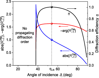
Figure 7. Dependence of the −1st reflection coefficient and of the diffraction efficiency on the angle of incidence. TM polarization,  SiO2 dielectric layer. Left vertical axis: reflection coefficient; blue line—absolute value, red line—negative phase (in radians). Right vertical axis: diffraction efficiency, black line.
  —the Littrow angle, 53.83°.
Download figure:
Standard image High-resolution image3.4. Influence of the protective dielectric layer
In practical applications, the metal grating has to be protected by a thin but hard enough dielectric layer, such as SiO2, as shown in figure 8.

Figure 8. Diffraction grating with a protective layer. The relative permittivity and the thickness of this layer are denoted as  and
and  , respectively.
Download figure:
Standard image High-resolution imageSince we do not want to overload this article with detailed numerical analysis of this structure, we present here only selected results of practical importance.
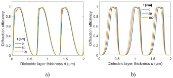
In figure 9 we show the diffraction efficiency of the grating in dependence of the bottom dielectric layer thickness (as in figure 4) for several values of the thickness of the SiO2 protective layer  for both TM and TE polarizations.
Figure 9. Diffraction efficiency of the grating without and with protective SiO2 layer of the thickness t. Other parameters as in figure 4. Blue line— , red—
 and yellow—
 (a) TM polarization, (b) TE polarization.
Download figure:
Standard image High-resolution image
Obviously, although the protective layer slightly modifies the shape of the curves, the maximum diffraction efficiency of the grating close to 100% is retained.
4. Conclusions
We presented a detailed electromagnetic analysis of a novel type of a very simple flat metal-dielectric grating with the (theoretical) 100% diffraction efficiency in the Littrow configuration. The grating is formed by a planar dielectric slab metalized at both sides, with periodic parallel slits opened in one of the metal layers. In order to keep the analysis as simple as possible, infinitely thin perfect metal (with either infinite conductivity or infinite negative permittivity) was considered. It has been shown that the retro-diffraction efficiency of 100% can be obtained for both TM and TE polarizations, although for different grating parameters. Very high diffraction efficiency can be obtained with a number of different grating arrangements. Reduced sensitivity to the variations of the thickness of the dielectric slab is obtained for the metal filling factors (the ratio between the width of the metal stripes and the grating period) of about 0.45 for the TM polarization and only about 0.045 for the TE polarization. High diffraction efficiency for the TE polarization can be reached with the filling factor of about 0.5 too, at the expense of an increased sensitivity to the dielectric slab thickness.
The optical energy stored within the dielectric slab between the metal layers is the larger, the larger is the metal filling factor of the grating. For values of  it is several times higher than in the incident and reflected waves. This fact has to be taken into account in the typical application of the grating as a wavelength-selective laser mirror [16]. It has also been indicated that at the Littrow configuration, the cross-section shape of the beam diffracted into the −1st reflected order is only very weakly modified, and there is essentially no Goos–Hänchen shift between the incident and diffracted beams. Thanks to a rather relaxed sensitivity of the grating to the incidence angle close to the Littrow configuration, the diffraction efficiency remains very high even for beams of the waist diameter of only a few tens of micrometres. These physical properties, together with a relative ease of fabrication, make the flat metal-dielectric grating discussed here a very promising candidate for applications as tuning grating mirrors for near-infrared lasers. For gold metal layers and SiO2 dielectric slab considered in this paper, the estimated maximum incident optical power density that the grating should be capable to bear without damage is of the order of 10 W cm−2. The total incident power can be increased by enlarging the grating area; relatively large gratings can be rather easily fabricated by using photolithographic patterning.
Acknowledgments
Financial support by the Technology Agency of the Czech Republic (Project TN01000008) and by the Czech Science Foundation (Project 1900062S) is greatly acknowledged.