

Abstract
The high power impulse magnetron sputtering (HiPIMS) discharge brings about increased ionization of the sputtered atoms due to an increased electron density and efficient electron energization during the active period of the pulse. The ionization is effective mainly within the electron trapping zone, an ionization region (IR), defined by the magnet configuration. Here, the average extension and the volume of the IR are determined based on measuring the optical emission from an excited level of the argon working gas atoms. For particular HiPIMS conditions, argon species ionization and excitation processes are assumed to be proportional. Hence, the light emission from certain excited atoms is assumed to reflect the IR extension. The light emission was recorded above a 100 mm diameter titanium target through a 763 nm bandpass filter using a gated camera. The recorded images directly indicate the effect of the magnet configuration on the average IR size. It is observed that the shape of the IR matches the shape of the magnetic field lines rather well. The IR is found to expand from 10 and 17 mm from the target surface when the parallel magnetic field strength 11 mm above the racetrack is lowered from 24 to 12 mT at a constant peak discharge current.
Export citation and abstract BibTeX RIS
1. Introduction
Magnetron sputtering is a highly successful thin film deposition technique that has been applied to a wide range of applications for the past few decades [1–3]. High power impulse magnetron sputtering (HiPIMS) is a variation of the magnetron sputtering technique where the discharge is operated at power densities of a few hundred kW cm−2 or higher, during short pulses of tens to hundreds of microseconds length [4, 5]. The pulsed discharge current density can peak at up to 10 A cm−2, when averaged over the cathode target surface. This enables a high electron density in the region close to the cathode target surface ( m−3) [1, 4, 6, 7], leading to an increased ionization of the working gas, and more importantly, of the atoms sputtered from the cathode target. The increased ionization of the sputtered species greatly enhances the control of the thin film growth, and consequently, improves the resulting thin film properties [8–10].
In a magnetron sputtering discharge, a dense plasma is maintained next to the cathode target by a static magnetic field. In the planar configuration a confining magnetic field is created by concentrically placing a central magnet and an outer edge magnet, with anti-parallel magnetization, behind the cathode target [1, 11]. The magnetic field forms a magnetic trap, which confines the electrons in the vicinity of the cathode target. This electron confinement translates into a region of enhanced electron density, and consequently, as most of the ionization is due to electron impact ionization, increased ionization, forming what we refer to as the ionization region (IR). The IR in a magnetron sputtering discharge, therefore, stands for the region where sputtered atoms and working gas atoms are most likely to be ionized. This region can be observed visually as a brightly glowing torus that sits adjacent to the target surface.
Despite its importance for the operation of a HiPIMS discharge, little is known about the extent of the IR. In a recent experimental work by Dubois et al [12], both the electron temperature and the electron density are found to drop exponentially with distance from the target surface. Another study by Kanitz et al [13], used an extended tunable diode laser absorption spectroscopy set-up to determine the spatial and temporal dynamics in HiPIMS discharges. They showed that the spatial distribution of the metastable argon atoms (Ar is confined below the magnetic null point (
 , the location where the magnetic field is zero, which was 22.5 mm in their case). Furthermore, they found the light emission from Ar+ ions to follow the magnetic field lines.
The IR is also a region of a strong temporal variation. An early temporally resolved optical emission spectroscopy (OES) study revealed the temporal variation in the plasma composition, as it was observed that the onset of the Ar emission coincided with the increase in the discharge current while the peak in the emission from the sputtered metal species occurs at a later time [14]. As a result, there is a separation in the arrival time at the substrate for the ions of the working gas and the ions of the film forming material. Time-resolved OES has also been applied to study the plasma dynamics of HiPIMS discharges [6, 15–18]. Five phases have been identified [4, 6]: (i) ignition, (ii) current rise–working gas ion sputtering, (iii) working gas depletion, (iv) plateau–self-sputtering, and (v) afterglow. Also, using OES, working gas rarefaction has been observed and shown to be rather significant in HiPIMS discharges [19–24]. Some of these works have reported the temporal evolution of the spatial distribution of the emission in front of the cathode target [15–17].
The strong gradients and the heterogeneity of the IR stand in clear contrast to the basic assumption of global models for HiPIMS discharges. One such example is the IR model (IRM) [25, 26]. The IRM is a volume-averaged global model of the plasma chemistry in a pulsed magnetron sputtering discharge. The modelled region in the IRM, and in other global models of the HiPIMS discharge, is limited to the IR, which in the model is defined as an annular cylinder with a rectangular cross-section and given outer (r1) and inner (r2) radius marking the racetrack region, and an axial extension  from the target surface [25, 27, 28]. Its shape can also be assumed to be half a torus with set radius, height, and width assuming both circular [29] and rectangular (linear) [30] targets.
In order to develop more precise global models for HiPIMS discharges, there is a need to understand the shape and the structure of the IR. Volume-averaging is still necessary for such models, in order to keep the character of a global model. Process parameters, on the other hand may have an important influence on the shape of the IR. One process parameter of particular importance in this regard is the magnetic field as it is responsible for the electron confinement.
Here, spectroscopic imaging is applied to determine the shape and size of the IR for various magnetic field configurations. Note, that when discussing the shape of the IR below, it refers to the time-averaged shape of the IR, blurring any structures from plasma instabilities.
In section 2 the experimental setup and the measurement method are described. Section 3 discusses the geometrical parameters determined for the IR, and the results are discussed in section 4. A summary of the findings is given in section 5.
2. Experimental apparatus and method
2.1. Methodology
We here suggest an indirect measurement to determine the size of the IR. For this, we assume the emission intensity of the Ar I line at λ = 763 nm to be a good measure for the argon ionization rate. The idea is based on the fact that the emission intensity at 763 nm is proportional to the population rate of the upper 4p[3/2]2 level (at 13.17 eV), with the correspondent lower one being the metastable 4s[3/2]2 level (at 11.54 eV). If the level populates proportionally to the ionization rate, the emission at 763 nm can be taken as a measure for the ionization rate.
First, let us discuss the population pathway of the 4p[3/2]2 level. For this, there are two principal possibilities, the direct population from ground state and the step-wise population via one of the 4s levels. To quantify the estimates, we take an argon model by Bultel et al [31] who lists cross sections from each of the four 4s levels and from the ground state to the combined (4p[3/2] , 4p[5/2]
 ) level, which contains the 4p[3/2]2 state. Considering the combined level is justified here as strong mixing can be expected within the 4p manifold. Figure 1 shows the rate coefficients for these processes. Considering that the density of the Ar 4s levels is typically at least two orders of magnitude below the ground state density in HiPIMS discharges [32, 33], for an electron temperature above 2 eV, direct population from the ground state is the dominant population mechanism. This finding agrees with the analysis by Stancu et al [34] (see appendix D in Stancu et al [34]).
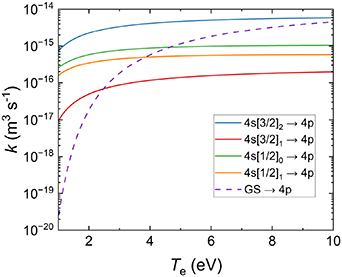
Figure 1. The rate coefficients for electron impact excitation from the ground state and from each of the four 4s levels to the combined (4p[3/2] , 4p[5/2]
 ) level, versus electron temperature.
Download figure:
Standard image High-resolution imageNext, we discuss the proportionality between the 4p[3/2]2 population and the electron impact ionization rate coefficient from the ground state. Figure 2 shows the ratio of the rate coefficients for electron impact excitation to electron impact ionization. One can see that for electron temperatures at 3 eV the rates are equal, and above 4 eV the ratio is rather flat. For HiPIMS discharges, electron temperatures above 4 eV have indeed been observed in modeling [32, 33, 35], and this is expected to represent the electron temperature next to the target surface. Experimentally, however, usually lower electron temperatures are determined, which is typically explained by the fact that they are measured at some distance from the target surface for various target materials [36–41]. Dubois et al [12] applied Thomson scattering measurements and determined the electron temperature to be 1.3 eV at 5 mm from a titanium target surface. This is lower than what has been observed by Langmuir probe measurements at 40 mm and 100 mm away from a titanium target, 3.5 eV [40] and 2 eV [41], respectively. In the most recent study by Held et al [42] the Langmuir probe is placed 8 mm above the target surface, parallel to the target surface, and the electron temperature is determined to be roughly 4 eV and agree very well with IRM calculations. The IRM calculations consistently give an electron temperature of 4 eV and higher for a discharge with a titanium target [34, 43]. So it is safe to assume that the electron temperature is around or above 4 eV during the pulse within the IR. We therefore conclude that the emission intensity from the 4p[3/2]2 level to the 4s[3/2]2 level is a good indicator for the presence of ionization, and therefore a good measure of the IR volume.

Figure 2. The ratio of the electron impact excitation rate coefficient for direct excitation to the combined (4p[3/2] , 4p[5/2]
 ) level from the ground-state argon atom and the electron impact ionization rate coefficient from the ground-state argon atom as a function of electron temperature.
Download figure:
Standard image High-resolution image2.2. Experimental details
The experiments were carried out in a custom-built cylindrical vacuum chamber (height 50 cm and diameter 45 cm) made of stainless steel, with a VTech (Gencoa Ltd, United Kingdom) magnetron assembly with a 4 inch (100 mm) diameter titanium target, installed. A base pressure of
  Pa was achieved using a turbo molecular pump backed by a roughing pump. Argon was used as the working gas and maintained at 1 Pa. The discharge was operated in HiPIMS mode. The pulses were 100 µs long, delivered by a pulsing unit (HiPSTER 1, Ionautics, Sweden), which in turn was fed by a regular DC power supply (1.5 kV and 2 A, Technix, France). Micrometer screws placed at the back of the magnetron assembly allow for accurate displacement of each magnet without breaking the vacuum. Here, optical emission spectrometery is applied to determine the shape and size of the IR for the same magnet configurations as explored experimentally by Hajihoseini et al [44]. Thus, seven magnet configurations have been systematically studied by varying the position of the center (C) and edge (E) magnets, namely, C0E0, C0E5, C0E10, C5E0, C5E5, C10E0, and C10E10. The numbers indicate the displacement of each of the magnets from the back of the target, in millimeters. For example, C10E0 means that the center (C) magnet is shifted back 10 mm away from the target backplate. The shifting of the magnets is shown schematically in figure 3(a). The edge (E) magnet has the north pole facing the target back side, while the C magnet is reversed. Except for the C10E10, the peak discharge current was maintained at about 40 A (
 A cm−2) by adjusting the discharge voltage figure 4. This is what we have referred to as the fixed peak current operating mode [44, 45]. The repetition frequency was adjusted as well to keep the averaged discharge power
  constant, when the magnetic configuration is varied.
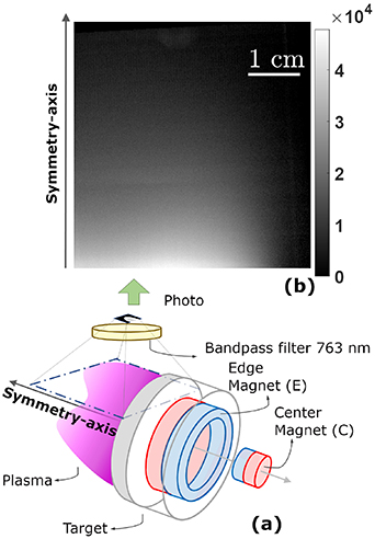
Figure 3. (a) The experimental setup showing the magnetron assembly and its magnets arrangement. The magnets show the C10E0 configuration. The optical arrangement is composed of an interferential filter and a gated camera. Note that due to the axis symmetry, it is sufficient that the camera captures one half of the discharge, the right side of the symmetry-axis. (b) Example of the raw captured image.
Download figure:
Standard image High-resolution image
Figure 4. The discharge (a) current and (b) voltage waveforms for each magnet configuration. The discharge was formed with argon at pressure of 1 Pa as the working gas and a 4 inch (100 mm) diameter titanium target. A gray semi-transparent box indicates the time period when the frames were taken.
Download figure:
Standard image High-resolution imageFigure 3(a) also shows the arrangement of the optical system with respect to the cathode target and the IR. A camera (VEO 710L, Phantom) was radially positioned 70 cm away from the axis normal to the target surface. The recorded light emission came from half of the torus-shaped IR, the half on the right side of the axis (figure 3(a)). The light then passed through a window (viewport). A photo lens (Nikkor 50 mm 1:1.2, Nikon, Japan) and an interferential bandpass filter centered on the 763 nm line (10 nm bandwidth) completed the arrangement. The camera was triggered with the onset of the pulse voltage and two recordings per pulse were captured with 45 µs and 5 µs of acquisition and readout time, respectively. The second image of each pulse was used for the analysis presented in the current study, recorded between 50 and 95 µs from the pulse initiation. This time range included the part with the high discharge currents that are characteristic for a HiPIMS discharge and therefore most interesting. The raw images had a size of  pixels and a resolution of 0.15 mm pixel−1.
For each magnetic field configuration, the camera recorded 13 images. The images displayed in this work are single frames, but the quantitative results presented are average values over all the sampled images, and the associated errors are the corresponding standard deviation. An example of a raw image is shown in figure 3(b). Each image was processed by inverse Abel transformation or Abel inversion [46], which yielded localized information on the light emission above the guard ring of the magnetron. By Abel inversion line-of-sight intensity measurements are transformed, to give information on the internal radial distribution of the emission from the plasma. The assumption of azimuthal symmetry around the symmetry axis holds since time variation due to spoke motion occur on a much shorter time scale (typically hundreds of ns).
3. Results
Figure 5, panels (a)–(g) depict the light emission from the 763 nm line in front of the target, for each magnet configuration (indicated with a label on each frame), after applying the inverse Abel transform. Note that these are single frame figures. A comparison of the results show that the varying magnet configurations lead to different shapes of the light emission zone and, therefore, varying size and shape of the IR. The lines in the false color map are iso-intensity lines, further highlighting the changes in shape with the magnetic topology. The light intensity is seen to be the strongest over the racetrack from where it decays with increasing distance from the racetrack. The bottom limit is the guard ring that blocks the first 3 mm above the Ti target surface.
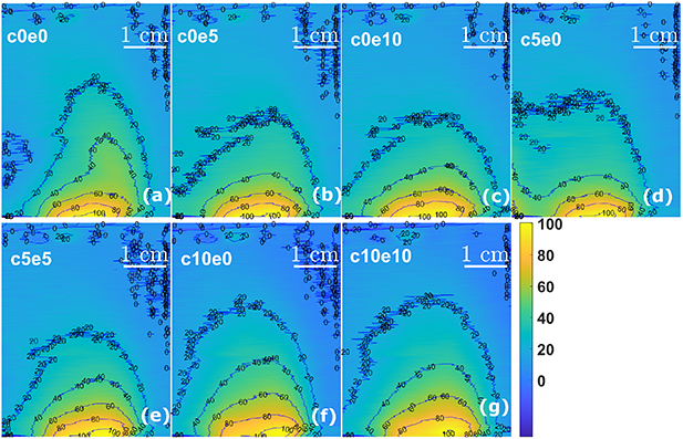
Figure 5. Images showing the light emission in front of the target after inverse Abel transformation. The numbers in black refer to the relative intensity compared to the brightest region in each frame. The light intensity is the strongest over the racetrack. The center magnet (C) and the edge magnet (E) displacement in millimeters correspond to numerical values in the labels (a) C0E0, (b) C0E5, (c) C0E10, (d) C5E0, (e) C5E5, (f) C10E0, and (g) C10E10.
Download figure:
Standard image High-resolution imageFigure 6 (left column) shows the normalized images of the data shown in figure 5, by its maximum pixel intensity, side by side with corresponding magnetic field line plots (right column) replotted from Hajihoseini et al [44]. The pixels in the images shown in the left column of figure 6 are in all cases normalized to their brightest intensity. The contour lines represent the iso-intensity every 10%.

Figure 6. The IR cross-section, left column, and magnet field line maps, right column, versus magnet configuration of (a) C0E0, (b) C0E5, (c) C0E10, (d) C5E0, (i) C5E5, (f) C10E0, and (g) C10E10. In all cases the intensity of the emission is normalized to their brightest intensity. The spatial extension away from the target surface (guard ring) is assumed to correspond to the line of half-intensity pixels relative to their maximum (border between the blue line and black background). The blue contour lines indicate the iso-intensity every 10%. The magnetic field strength is displayed for all plots of the magnetic field lines at r = 25 mm and z = 10 mm.
Download figure:
Standard image High-resolution imageIn this study we define the outer border of the IR at the location where the intensity falls to 50% of the maximum value. Our choice of a 50% reduction of light intensity as defining the limit of the IR is not based on any strict argument. Another limit, say, 60% could be equally motivated and would give a larger IR. However, what we here are interested in is not the exact IR size, but to investigate the trends of the IR with the magnetic field. For this purpose our specific choice of 50% is not crucial.
Assuming this cut-off value, various geometrical parameters of the IR can be determined. Figure 7(a) shows schematically how the axial extension of the IR from the guard ring  , the width of the IR at the guard ring
  , and the cross-sectional area of the IR above the guard ring
  , are determined from the data in figure 6. We used the primed parameters to highlight that they are determined from the guard ring. Table 1 summarizes the determined values for
  ,
,  ,
,  , the radial magnetic field strength (
 ), the location of the magnetic null point from the guard ring
  , and the pulse power [45, 47]. The
  is in the range from
  mm to
mm to  mm corresponding to the axial extension of the IR from the target surface
  in the range from
  mm to
mm to  mm. The
  is found to be in the range
  mm to
mm to  mm.
mm.  was measured 11 mm above the racetrack (or 8 mm above the guard ring) and
  is the location at which the magnetic field strength becomes null on the symmetry-axis of the magnetron (figure 7(b)). Finally, the pulse power is calculated from the data presented in figure 4.
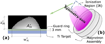
Figure 7. (a) An example of the IR cross section within quantitative values as axial extension  (along z-axis, symmetry-axis) in mm, width
  (along the r-axis) in mm, and the area
  in mm2. The
  and
and  are measured above the guard ring. (b) Sketch of the IR volume.
Download figure:
Standard image High-resolution imageTable 1. Parameters derived from the optical measurements: the IR axial extension  , its width
  above the guard ring, the
  , the magnet configuration, the radial magnetic field strength
  (at the racetrack 11 mm above the target), the location of the magnetic null point
  , and the pulse power.
| Magnet |

|

|

|

|

| Pulse power |
|---|---|---|---|---|---|---|
| configuration | (mm) | (mm) | (mm2) | (mT) | (mm) | (kW) |
| C0E0 |

|

|

| 23.8 | 63 |

|
| C0E5 |

|

|

| 21.7 | 67 |

|
| C0E10 |

|

|

| 21.3 | 71 |

|
| C5E0 |

|

|

| 18.1 | 50 |

|
| C5E5 |

|

|

| 16.1 | 56 |

|
| C10E0 |

|

|

| 13.7 | 40 |

|
| C10E10 |

|

|

| 11.1 | 49 |

|
Figure 8 shows the axial extension of the IR  , the width of the IR
  , and the cross sectional area of the IR
  , as a function of the radial magnetic field strength
  . The measurements of each of the parameters were independent and all of them show similar behavior, a linear-like trend with a negative slope for weak magnetic fields
  mT), and a breaking of this trend for stronger fields
  mT). Hence, strengthening the magnetic field up to about 18 mT shrinks the IR. Beyond 18 mT, the total
  area seems to stay almost constant. This is because the axial extension
  decreases with increased magnetic field to a minimum at 18 mT and then saturates with further increase in magnetic field (except for the C0E0 case, which we discuss later). Also the width
  shows a similar behavior; decreases at first with increasing magnetic field and then saturates for magnetic field strengths above 18 mT. The largest axial extension of the IR
  , the largest width of the IR
  above the guard ring, and the biggest cross sectional area
  are all observed for the weakest magnetic field obtained with the C10E10 configuration of the magnets.

Figure 8. The (a) axial extension of the IR above the guard ring  , (b) the width of the IR at the guard ring
  , and (c) the cross sectional area of the IR above the guard ring
  as a function of the radial magnetic field strength (table 1). The dashed lines are a guide for the eye.
Download figure:
Standard image High-resolution image4. Discussion
4.1. Shape of the IR
It can be clearly seen in figure 6 that the shape of the magnetic field lines matches the contours of the IR. This observation can be explained in terms of electron confinement. Due to a high electron conductivity along the magnetic field lines, the electron properties, notably the density and temperature, are close to being constant along a magnetic field line. Conversely, the electron conductivity across the magnetic field lines is limited [48–50], so that electron properties can change drastically in the direction orthogonal to the magnetic field lines. It is therefore understandable that the shape of the IR closely follows the magnetic field lines.
4.2. Electron confinement
Electrons in a magnetic field gyrate around the field lines with a gyro radius ( ) that is inversely proportional to the magnetic field strength
  , i.e.
  [51]. The classical (collisional) cross-B transport speed is proportional to
  [4, 48]. The electron mobility across the magnetic field lines therefore changes with the magnetic field strength [4, 48]. We see in figure 8(a) that in the range
  mT, the IR axial extension (
 ) is close to being inversely proportional to
  , i.e. proportional to
  . Therefore, the shrinking size of the IR should be due to a reduction in electron mobility from a stronger
  .
.
Figure 8(b) shows that the width of the IR exhibits the same behavior as the axial extension. It has been suggested and confirmed experimentally in a dc magnetron sputtering discharge that the width of the racetrack region  scales as
  [52], which supports our hypothesis that the shrinking size of the IR is related to the electron mobility.
For a decreasing  , a higher voltage is necessary to sustain the discharge, as can be seen in figure 4(b). Note that the highest discharge voltage was needed for our weakest magnetic field, the C10E10 configuration, as seen in figure 4(a), but the peak discharge current could not reach 40 A. In the extreme case of no magnetic field, i.e. in the case of dc diode sputtering, electrons are not confined at all. What is found with lower
  , in figure 6, is therefore the beginning of the 'loss of electron confinement'. The IR, its shape and size is therefore intrinsically connected to the magnetic trap.
For a magnetic field strength  in the range 18 to 22 mT, the IR axial extension
  stays almost constant as the magnetic field strength is increased. The plasma volume thus shrinks with increased magnetic field strength until it reaches a certain limit. The IR does not shrink below this limit when the magnetic field is further increased. This could indicate that the electron confinement is not further improved by strengthening the magnetic field B. The pulse power barely changes for those conditions, as can be seen in table 1, meaning that the electron density and temperature might be roughly the same.
For the strongest magnetic field,  mT, corresponding to the magnet configuration C0E0, the IR axial extension
  increases and thereby deviates from the reported trend, as seen in figure 8(a). Note also its large errors bar. The nature of the discharge might here change due to enhanced instabilities induced by electric and magnetic cross field (
 ) drifts or spokes [12, 13, 53]. Note that on shorter time scales than those used to record the images, one can observe plasma instabilities, so called spokes. They can be observed with gated cameras looking laterally and axially onto the discharge [50, 53, 54] and through simulations [55, 56]. Such instabilities further complicate the description of the IR. It is important to point out that the IR width
  and cross-sectional area
  do not show such a deviation from saturation (figures 8(b) and (c)). Regarding the symmetry of the IR, Kanitz et al [13] observed something similar to the one presented in this study. They observed a distribution of metastable argon atoms Ar
 , with the difference that they see it beyond the
  , indicating their diffusion [57].
4.3. Spatial variations of 

We can think of the electrons, to a first approximation, as being trapped along the magnetic field lines, bouncing between the magnetic mirrors at both ends of the magnetic field lines, as these approach the target. This means that we can assume the same electron energy distribution (EEDF) along each flux tube. This is why we observe an agreement between the optical emission and the magnetic field line structure as shown in figure 6. We now consider a cloud of electrons within such a flux tube. The question is what the temporal evolution of the EEDF is during their drift away from the target. For simplicity we consider an initially Maxwellian EEDF. For this electron population the electron temperature is determined by the opposing processes of Ohmic heating and energy loss by collisions. The heating rate is proportional to the electric field E, and is therefore stronger close to the target surface, and drops with the distance away from the target surface. The cooling rate is proportional to the working gas density and remains more constant with increasing distance from the target. This means that at a certain distance the cooling mechanism takes over. If the population remains Maxwellian the drifting electron cloud would be characterized by an electron temperature which gradually decreases as it moves away from the target, which has indeed been observed experimentally, as discussed above [12].
Regarding the variation of electron density and electron temperature with distance from the target surface, Dubois et al [12] investigated the drop in electron density and electron temperature above the racetrack using Thomson scattering measurements. The spatial variation in electron density was found to show a bi-exponential dependence while the variation in electron temperature could be described by a simple exponential function. For a pulse length of 70 µs, an argon working gas pressure of 1 Pa, and a peak discharge current of 40 A, for the C5E5 magnetic configuration, they determined the electron density 3 mm above the guard ring to be  m−3 and to fall to half of this value at roughly 12 mm above the guard ring and drop by about 70% at roughly 22 mm above the guard ring. This is roughly of the same distance as what we determine to be the axial extension of the IR using OES. They also found the electron temperature to drop, from 1.3 eV 3 mm above the guard ring, to about 0.7 eV 40 mm above the guard ring. However, in similar conditions, other investigations have determined higher electron temperatures,
  eV (8 mm from the target surface) [42], 3.5 eV (40 mm from the target surface) [40] and 2 eV (100 mm from target surface) [41], thus higher than measured by Thomson scattering [12]. Also, just above the sheath, facing the target, particle-in-cell Monte Carlo collision simulation results show electron temperature of ∼7 eV [55], where most of the ionization is suggested to occur [42, 58]. Then, it is expected that the electron temperature drops across the IR. The effect of a drop in electron temperature with increasing distance from the cathode, by collisions with the atoms, would be that the IR appears larger in images recording the emission from the 4p level, than it actually is. In other words, if the electron temperature drops below 3 eV, the electron impact excitation rate coefficient will become larger than the electron impact ionization rate coefficient, and the excitation and ionization cannot be considered proportional any more, as can be seen in figure 2. Consequently, the IR will be smaller than presented in figure 6. Nevertheless, in such case, the trends seen in figure 8 will remain the same. Notice all iso-contours (blue lines) seen in figure 6 follow the same trend. Further out in the IR, where electron temperatures are lower compared to the target vicinity, the ionization rate can therefore be expected to be low. Assuming an electron temperature of 1 eV at the here-determined border of the IR, we expect an excitation rate that is a factor of 10 to 20 higher per ionization rate, compared to the target vicinitiy with electron temperatures
  eV. Combining this with the 50% cut-off in emission intensity at this border, we note that the ionization rate at the here-determined border will be factor of 20–40 lower compared to the near-target vicinity.
4.4. IR models
The magnet configurations explored here were the same as in the experimental work of Hajihoseini et al [44], where the ionized flux fraction and deposition rate was reported for the various magnet configurations, while keeping the average power constant, by either maintaining fixed discharge voltage or fixed peak discharge current. The discharges explored by Hajihoseini et al have been studied extensively, including exploring the influence of magnetic field on the discharge current, the electron density and the ionization probability [35], to determine the transport parameters of the neutrals and ions of the sputtered species [59], as well as demonstrate how to minimize variations of the flux parameters, the deposition rate and the ionized flux fraction, as the target erodes [45]. The size of the IR is an input parameter when modeling the HiPIMS discharge, using models such as the IR model [26, 27]. When modeling the HiPIMS discharge, the IR has been assumed to extend up to several tens of millimeters from the cathode target [25, 60]. In the IRM, to calculate the plasma chemistry in a volume given by a rectangular torus with radii r1 and r2, which set the width of the racetrack  . In the IRM study of the discharges explored using the same magnetron assembly and cathode, the IR was assumed to be 28 mm wide and extend 25 mm away from the target surface [27]. The results presented in figure 8 show the axial extension
  to be in the range 7–14 mm (i.e. 10–17 mm from the target surface) and the width of the IR at the guard ring
  to be 23–29 mm. The volume of the IR is
  , with
  25 mm [44] as the radial position of the racetrack from the center of the target, is here determined to be 2.1–
 m3, compared to
  m3 used in the IRM calculations [27]. We note that the measured volume from this work matches well with the assumed volume of the IR. However, for more precise global models of the HiPIMS discharge, the shape of the IR and the gradient in electron temperature and density are likely parameters to be optimized in future developments.
5. Summary
We studied the extension of the IR in a HiPIMS discharge as a function of the magnetic field strength and configuration. For this, images were taken within the second half of a discharge pulse using a fast camera and a band pass filter (763 nm) to collect the emission due to the transition from an excited level in the 4p manifold (4p[3/2]2) at 13.17 eV of the Ar atom to a metastable state in the 4s manifold at 11.54 eV (4s[3/2]2). We assume that this transition probes the extent of the IR. After inverse Abel transformation, or Abel inversion, the resulting images exhibit a bright region near the target which we identify as the IR. We assume the edge of the IR to be where the light intensity has fallen to less than half of its maximum intensity.
We show that the shape of the IR closely follows those of the magnetic field lines which are determined by the location of the permanent magnets at the back of the cathode. The axial extent of the IR,  , depends inversely on the strength of the magnetic field, as expected for gyrating electrons. It varies from 10 to 17 mm. The width of the IR,
  , and the cross sectional area,
  , show similar behavior with increasing
  , i.e. a linear decrease for
  mT, and constant values in the range 18.1 mT
  mT.
mT.
Acknowledgment
The authors acknowledge Charles Ballage for the help with inverse Abel transform code. This work was partially funded by the Icelandic Research Fund (Grant No. 196141), the Swedish Research Council (Grant No. VR 2018-04139), and the Swedish Government Strategic Research Area in Materials Science on Functional Materials at Linköping University (Faculty Grant SFO-Mat-LiU No. 2009-00971).
Data availability statement
All data that support the findings of this study are included within the article (and any supplementary files).