


1. Introduction
The invention of the chirped pulse amplification (CPA) technique (Strickland & Mourou Reference Strickland and Mourou1985) in the mid-1980s allowed the rapid growth of the laser power beyond the terawatt (TW) level. The petawatt (PW) threshold was exceeded at the end of the 20th century(Perry et al. Reference Perry, Pennington, Stuart, Tietbohl, Britten, Brown, Herman, Golick, Kartz and Miller1999). Currently, the record power is for the ELI-NP 10 PW laser (Tanaka et al. Reference Tanaka, Spohr, Balabanski, Balascuta, Capponi, Cernaianu, Cuciuc, Cucoanes, Dancus and Dhal2020), with another $10\ \mathrm {PW}$ laser near completion at ELI Beamlines. Current worldwide activities concerning PW laser systems and further envisions to attain ${>}100\ \mathrm {PW}$
 lasers are summarized in Danson et al. (Reference Danson, Haefner, Bromage, Butcher, Chanteloup, Chowdhury, Galvanauskas, Gizzi, Hein and Hillier2019) and Li, Kato & Kawanaka (Reference Li, Kato and Kawanaka2021).
Since laser power increases by either increasing the energy or reducing the pulse duration, a single-cycle pulse was proposed (Mourou et al. Reference Mourou, Chang, Maksimchuk, Nees, Bulanov, Bychenkov, Esirkepov, Naumova, Pegoraro and Ruhl2002; Bulanov et al. Reference Bulanov, Esirkepov, Kamenets and Pegoraro2006; Voronin et al. Reference Voronin, Zheltikov, Ditmire, Rus and Korn2013). Post-compression of CPA systems leads to near-single-cycle pulses by self-phase modulation in hollow-core fibres, although the energy is at the millijoule level (Böhle et al. Reference Böhle, Kretschmar, Jullien, Kovacs, Miranda, Romero, Crespo, Morgner, Simon and Lopez-Martens2014; Ouillé et al. Reference Ouillé, Vernier, Böhle, Bocoum, Jullien, Lozano, Rousseau, Cheng, Gustas and Blumenstein2020). A second technique producing near-single-cycle pulses is optical parametric CPA, by which a $4.5 \ \mathrm {fs}$ , $16 \ \mathrm {TW}$
 pulse has been reported (Rivas et al. Reference Rivas, Borot, Cardenas, Marcus, Gu, Herrmann, Xu, Tan, Kormin and Ma2017). Reducing the pulse duration is the primary goal of ELI-ALPS, where a $17 \ \mathrm {fs}$
 , $2 \ \mathrm {PW}$
 laser is under development (Osvay et al. Reference Osvay, Börzsönyi, Cao, Cormier, Csontos, Jójárt, Kalashnikov, Kiss, López-Martens and Tóth2019). Thus, at a given laser power, reduction of the pulse duration leads to a linear reduction of the energy, consequently the minimum laser energy for a single-cycle pulse.
However, it is most desired to reach the highest laser intensity rather than power. The quadratic dependency of the intensity on the inverse of the focal spot radius points to an emphasis on a reduced focal spot. More than two decades ago, a theoretical estimation of the minimum focal spot diameter (Sales Reference Sales1998) suggests a value of $4 {\rm \pi}^{-2} \lambda$ , where $\lambda$
 is the laser wavelength. A vectorial diffraction approach was adopted (Richards, Wolf & Gabor Reference Richards, Wolf and Gabor1959; April & Piché Reference April and Piché2010) to describe a focal spot smaller than the wavelength. The benefit of the vectorial representation is that Maxwell's equations are satisfied at any point in space, and analytical expressions for the electric and magnetic field components can be calculated (April & Piché Reference April and Piché2010; Jeong et al. Reference Jeong, Weber, Le Garrec, Margarone, Mocek and Korn2015; Salamin Reference Salamin2015). Experimental implementation of a tight-focusing scheme by a parabola with f-number $f_N$
 (the ratio of focal length $f$
 to beam diameter $D$
 ) of $0.6$
 claims focusing of a $45 \ \mathrm {TW}$
 laser to a focal spot of ${\sim } 0.8 \ \mathrm {\mu } \mathrm {m}$
 in diameter, leading to an intensity of ${\sim } 10^{22} \ \mathrm {W}\ \mathrm {cm}^{{-2}}$
 (Bahk et al. Reference Bahk, Rousseau, Planchon, Chvykov, Kalintchenko, Maksimchuk, Mourou and Yanovsky2004), where a similar intensity is achieved by focusing a $0.3 \ \mathrm {PW}$
 laser using a parabola of $f_N = 1.3$
 (Pirozhkov et al. Reference Pirozhkov, Fukuda, Nishiuchi, Kiriyama, Sagisaka, Ogura, Mori, Kishimoto, Sakaki and Dover2017).
Apart from the usually employed linearly polarised (LP) lasers, radially polarised (RP) and azimuthally polarised (AP) lasers draw much interest of several research groups, employing multi-PW lasers for electron (Salamin Reference Salamin2010a; Payeur et al. Reference Payeur, Fourmaux, Schmidt, MacLean, Tchervenkov, Légaré, Piché and Kieffer2012) and proton/ion (Salamin Reference Salamin2010a; Li et al. Reference Li, Salamin, Galow and Keitel2012; Ghotra & Kant Reference Ghotra and Kant2015) acceleration. Let us define the laser propagation direction to be along $\hat {\boldsymbol {x}}$ . In cylindrical coordinates, a RP plane wave satisfies $E_r \hat {\boldsymbol {r}} = c B_{\phi } \hat {\boldsymbol {\phi }}$
 everywhere, where $E_r \hat {\boldsymbol {r}}$
 is the radial electric field component, $B_{\phi } \hat {\boldsymbol {\phi }}$
 is the azimuthal magnetic field component and $c$
 is the speed of light in vacuum. For an AP laser, the electric and magnetic field components are interchanged. However, under tight-focusing conditions the relation $E_r \hat {\boldsymbol {r}} = c B_{\phi } \hat {\boldsymbol {\phi }}$
 breaks down due to the appearance of a longitudinal electric field component $E_x \hat {\boldsymbol {x}}$
 for a RP laser and a longitudinal magnetic field component $B_x \hat {\boldsymbol {x}}$
 for an AP laser (Salamin Reference Salamin2006, Reference Salamin2010b; Jeong et al. Reference Jeong, Bulanov, Weber and Korn2018). Compared with LP lasers, both RP and AP lasers were found experimentally to give a smaller focal spot (Dorn, Quabis & Leuchs Reference Dorn, Quabis and Leuchs2003; Cheng et al. Reference Cheng, Zhou, Xia, Li, Yang and Zhou2015), in agreement with the elongated electric field distribution for a LP laser (Jeong et al. Reference Jeong, Bulanov, Weber and Korn2018).
When the concept of a single-cycle laser is combined with the tight-focusing technique, then the $\lambda ^{3}$ regime is obtained, where for a certain laser power one can use minimal energy to achieve the highest intensity (Mourou et al. Reference Mourou, Chang, Maksimchuk, Nees, Bulanov, Bychenkov, Esirkepov, Naumova, Pegoraro and Ruhl2002). The $\lambda ^{3}$
 pulses offer potential unique capabilities for atomic and molecular physics (Brabec & Krausz Reference Brabec and Krausz2000), electron–laser collisions (Tamburini, Keitel & Di Piazza Reference Tamburini, Keitel and Di Piazza2014b) and relativistic nanophotonics (Cardenas et al. Reference Cardenas, Ostermayr, Di Lucchio, Hofmann, Kling, Gibbon, Schreiber and Veisz2019), where such pulses may open up the investigation of a qualitatively new regime. If the $\lambda ^{3}$
 regime is applied to a $100 \ \mathrm {PW}$
 laser, then an intensity exceeding $10^{25} \ \mathrm {W}\ \mathrm {cm}^{{-2}}$
 will be achieved. For comparison, a record intensity of ${\sim } 10^{23} \ \mathrm {W}\ \mathrm {cm}^{{-2}}$
 has been recently reported for a ${\sim }4 \ \mathrm {PW}$
 laser (Yoon et al. Reference Yoon, Kim, Choi, Sung, Lee, Lee and Nam2021). Although generation of $\lambda ^{3}$
 pulses by optical means is challenging, this can also be realised by plasma-based techniques (Mourou et al. Reference Mourou, Mironov, Khazanov and Sergeev2014; Tamburini et al. Reference Tamburini, Di Piazza, Liseykina and Keitel2014a). Notably, the self-generation of such pulses has been observed in three-dimensional simulations during the interaction of a laser pulse with a foil target (Tamburini et al. Reference Tamburini, Liseykina, Pegoraro and Macchi2012).
The ultra-intense $\lambda ^{3}$ regime is capable of providing a plethora of particles, such as $\gamma$
 -photons, leptons (electrons ($\mathrm {e}^{-}$
 ) and positrons ($\mathrm {e}^{+}$
 )) and hadrons (protons ($\mathrm {p}^{+}$
 ) and/or heavy ions ($\mathrm {i}^{+}$
 )) (Mourou, Tajima & Bulanov Reference Mourou, Tajima and Bulanov2006). Although $\gamma$
 -photons are achievable even by near-PW-class lasers, high laser to $\gamma$
 -photon energy conversion efficiency, $\kappa _\gamma$
 , is important for applications in photonuclear reactions (Nedorezov, Turinge & Shatunov Reference Nedorezov, Turinge and Shatunov2004), astrophysical studies (Rees & Mészáros Reference Rees and Mészáros1992; Bulanov et al. Reference Bulanov, Esirkepov, Kando, Koga, Kondo and Korn2015; Philippov & Spitkovsky Reference Philippov and Spitkovsky2018; Aharonian et al. Reference Aharonian, An, Axikegu, Bai, Bai, Bao, Bastieri, Bi, Bi and Cai2021) and study of the extremely high energy density of materials science (Eliasson & Liu Reference Eliasson and Liu2013).
At laser intensities of ${\sim }10^{24}\ \mathrm {W}\ \mathrm {cm}^{{-2}}$ the multi-photon Compton scattering process dominates the $\gamma$
 -photon emission (Ridgers et al. Reference Ridgers, Brady, Duclous, Kirk, Bennett, Arber and Bell2013; Lezhnin et al. Reference Lezhnin, Sasorov, Korn and Bulanov2018; Younis et al. Reference Younis, Davidson, Hafizi and Gordon2021). During that process, a hot electron/positron is scattered after collision with the incident laser field, its velocity and direction values change and a scattered $\gamma$
 -photon is produced. The process is summarised as $\mathrm {e}^{{\pm }} + N \omega _l \rightarrow \mathrm {e}^{{\pm }} + \omega _\gamma$
 , where $\omega _l$
 is the central laser frequency, $\omega _\gamma$
 is the scattered $\gamma$
 -photon frequency and $N \gg 1$
 is the number of laser photons lost.
The Schwinger field represents the field required for the vacuum to break into an $\mathrm {e}^{-}$ –${\rm e}^{+}$
 pair, and it is given by $E_S = m_e^{2} c^{3} / (e \hbar ) \approx 1.3 \times 10^{18}\ \mathrm {V}\ \mathrm {m^{-1}}$
 , where $m_e$
 is the electron rest mass, $\hbar$
 is the reduced Planck constant and $e$
 is the elementary charge (Berestetskii, Lifshitz & Pitaevskii Reference Berestetskii, Lifshitz and Pitaevskii1982). The probability that a $\gamma$
 -photon will be emitted through multi-photon Compton scattering depends on the parameter (Ritus Reference Ritus1970)

where $\gamma _e$ is the electron/positron Lorentz factor of momentum $\boldsymbol {p}$
 prior scattering and ${\boldsymbol {B}}$
 and ${\boldsymbol {E}}$
 are the magnetic and electric fields at the position of the electron. For high $\kappa _\gamma$
 the condition $\chi _e \gg 1$
 must be met (Nakamura et al. Reference Nakamura, Koga, Esirkepov, Kando, Korn and Bulanov2012; Ridgers et al. Reference Ridgers, Brady, Duclous, Kirk, Bennett, Arber, Robinson and Bell2012). Although the emission model used (Ridgers et al. Reference Ridgers, Brady, Duclous, Kirk, Bennett, Arber and Bell2013) breaks down for ${\alpha \chi _e^{2/3} > 1 }$
 (Ritus Reference Ritus1970; Ilderton Reference Ilderton2019; Narozhny Reference Narozhny1979; Podszus & Di Piazza Reference Podszus and Di Piazza2019), where $\alpha = e^{2} / (4 {\rm \pi}\varepsilon _0 \hbar c)$
 is the fine structure constant and $\varepsilon _0$
 is the vacuum permittivity, it requires laser intensities significantly higher than those used in the present work.
The $\mathrm {e}^{-}$ –$\mathrm {e}^{+}$
 pair generation mechanism discussed in § 3 is the multi-photon Breit–Wheeler process (Ehlotzky, Krajewska & Kamiński Reference Ehlotzky, Krajewska and Kamiński2009), summarised as ${ \omega _\gamma + N \omega _l \rightarrow \mathrm {e}^{{-}} + \mathrm {e}^{{+}} }$
 . Here, a large number of laser photons interact with a high-energy $\gamma$
 -photon generated earlier through multi-photon Compton scattering, then generatinh an $\mathrm {e}^{-}$
 –$\mathrm {e}^{+}$
 pair. The probability of a $\gamma$
 -photon producing a pair is governed by the parameter (Ritus Reference Ritus1970)

where $\hat {\boldsymbol {p}}$ is the unit vector of the $\gamma$
 -photon momentum.
The high fields available from multi-PW lasers have attracted interest in $\gamma$ -photon generation. An electron co-propagating with the laser field produces neither $\gamma$
 -photons nor $\textit {e}$
 –$\mathrm {e}^{+}$
 pairs due to the opposite contribution of the electric and magnetic terms in (1.1). However, in a realistic laser–foil experiment scenario the laser field is reflected on the foil front surface, changing its orientation and therefore enabling generation of $\gamma$
 -photons (Zhidkov et al. Reference Zhidkov, Koga, Sasaki and Uesaka2002; Koga, Esirkepov & Bulanov Reference Koga, Esirkepov and Bulanov2005; Gu et al. Reference Gu, Klimo, Bulanov and Weber2018). Another early approach toincreasing the $\gamma$
 -photon yield suggested the use of two counter-propagating pulses (Bell & Kirk Reference Bell and Kirk2008; Kirk, Bell & Arka Reference Kirk, Bell and Arka2009; Luo et al. Reference Luo, Zhu, Zhuo, Ma, Song, Zhu, Wang, Li, Turcu and Chen2015; Grismayer et al. Reference Grismayer, Vranic, Martins, Fonseca and Silva2016). This scheme was later generalised in the use of multiple laser beams (Vranic et al. Reference Vranic, Grismayer, Fonseca and Silva2016; Gong et al. Reference Gong, Hu, Shou, Qiao, Chen, He, Bulanov, Esirkepov, Bulanov and Yan2017). The geometry of the target itself was also proven to be crucial, as the formation of a pre-plasma enhanced $\gamma$
 -photon formation (Lezhnin et al. Reference Lezhnin, Sasorov, Korn and Bulanov2018; Wang et al. Reference Wang, Hu, Zhang, Gu, Zhao, Zuo and Zheng2020b). Other schemes employing microfabrication of targets taking advantage of the reflected laser field have also been investigated (Ji, Snyder & Shen Reference Ji, Snyder and Shen2019; Zhang et al. Reference Zhang, Wu, Huang, Lan, Liu, Wu, Yang, Zhao, Zhu and Luo2021). In addition to the all-optical approach, the combination of a sub-PW laser beam with high-energy electrons has been considered (Magnusson et al. Reference Magnusson, Gonoskov, Marklund, Esirkepov, Koga, Kondo, Kando, Bulanov, Korn and Bulanov2019).
The theoretical framework for the absorption of the energy of a plane wave by electrons and ions of a foil target is described byVshivkov et al. (Reference Vshivkov, Naumova, Pegoraro and Bulanov1998), although ignoring the energy share of generated $\gamma$ -photons and consequently the effect of $\mathrm {e}^{-}$
 –$\mathrm {e}^{+}$
 pairs. In (17) of Vshivkov et al. (Reference Vshivkov, Naumova, Pegoraro and Bulanov1998), the target thickness, $l$
 , is connected to the electron number density, $n_e$
 , through

where $\epsilon _0$ is the normalised areal density and $n_{cr} = \varepsilon _0 m_e \omega ^{2} /e^{2}$
 is the critical electron number density. The optimum condition for coupling the plane wave to the target is obtained for $\epsilon _0 = a_0$
 , where $a_0 = e E / (m_e c \omega _l)$
 is the dimensionless amplitude. For $\epsilon _0 \ll a_0$
 , relativistic transparency of the target results in weak coupling of the laser to the target, whilst for $\epsilon _0 \gg a_0$
 , the laser field is strongly reflected by the target front surface.
Equations (32) and (33) of Vshivkov et al. (Reference Vshivkov, Naumova, Pegoraro and Bulanov1998) give the ratio of the reflected (at an angle $\theta _0$ with the target normal) to incident wave amplitude (complex reflectivity) for an s-polarised laser, $r^{s} = \varepsilon _0 / [\mathrm {i} \cos (\theta _0)+\varepsilon _0]$
 , and a p-polarised laser, $r^{p} = \varepsilon _0 \cos (\theta _0) / [\mathrm {i}+\varepsilon _0 \cos (\theta _0)]$
 , respectively. In an AP laser, $E_x$
 is always zero; in contrast, in a RP laser, $E_x$
 increases by reducing the f-number and dominates in the tight-focusing scheme. Therefore, the electric field vectors are oscillating longitudinally and transversely with respect to the target surface for normally incident ($\theta _0 = 0 ^{\circ }$
 ) AP and RP lasers, respectively. Therefore, there is a qualitative analogy of the electric field oscillation direction of $s$
 -polarised and $p$
 -polarised lasers incident at $\theta _0 = 90^{\circ }$
 with AP and RP lasers incident at $\theta _0 = 0^{\circ }$
 . As a result, for the tight-focusing scheme, an AP laser is reflected stronger than a RP laser. Up to this point, we have discussed the physical processes enabling us to study the interaction of an ultra-relativistic $\lambda ^{3}$
 laser with a solid target via particle-in-cell (PIC) simulations.
One aspect not addressed in PIC simulation studies is the further interactions of multi-MeV-energy particles with the surrounding material, either the vacuum chamber itself or a secondary target. Particle-in-cell-produced particles generate electrons through ionisation (Landau Reference Landau1944) but also $\mathrm {e}^{-}$ –$\mathrm {e}^{+}$
 pairs through pair production in the Coulomb field of nuclei (Bethe & Heitler Reference Bethe and Heitler1934) and/or atomic electrons (Wheeler & Lamb Reference Wheeler and Lamb1939). Post-PIC $\gamma$
 -photons may result from ionisation, $\mathrm {e}^{-}$
 –$\mathrm {e}^{+}$
 pair production, Bremsstrahlung emission (Koch & Motz Reference Koch and Motz1959; Aichelin Reference Aichelin1991), photonuclear reactions (Compton Reference Compton1923), nuclear interactions with heavy ions (Aichelin Reference Aichelin1991), Rayleigh and/or Compton scattering (Compton Reference Compton1923) or any combination thereof.
Furthermore, neutrons, protons, ions and nuclides are produced through photonuclear reactions (Hayward Reference Hayward1970), electronuclear reactions (Budnev et al. Reference Budnev, Ginzburg, Meledin and Serbo1975) and nuclear interactions with heavy ions (Aichelin Reference Aichelin1991). These interactions are simulated by the Monte Carlo (MC) particle transport code FLUKA (Böhlen et al. Reference Böhlen, Cerutti, Chin, Fassò, Ferrari, Ortega, Mairani, Sala, Smirnov and Vlachoudis2014; Battistoni et al. Reference Battistoni, Boehlen, Cerutti, Chin, Esposito, Fassò, Ferrari, Lechner, Empl and Mairani2015) which can estimate the radioactive nuclides produced and the energy spectra of the post-PIC-generated particles. These estimations are useful in nuclear waste management (199 1998), positron annihilation lifetime spectroscopy (Audet et al. Reference Audet, Alejo, Calvin, Cunningham, Frazer, Nersisyan, Phipps, Warwick, Sarri and Hafz2021), $\mathrm {e}^{-}$ –$\mathrm {e}^{+}$
 plasma studies (Chen et al. Reference Chen, Meyerhofer, Wilks, Cauble, Dollar, Falk, Gregori, Hazim, Moses and Murphy2011; Sarri et al. Reference Sarri, Poder, Cole, Schumaker, Di Piazza, Reville, Dzelzainis, Doria, Gizzi and Grittani2015) and nuclear medicine (Schneider et al. Reference Schneider, Agosteo, Pedroni and Besserer2002).
This paper starts with a description of our numerical solution for the laser field under the tight-focusing scheme as described in Jeong et al. (Reference Jeong, Weber, Le Garrec, Margarone, Mocek and Korn2015) (for LP lasers) and Jeong et al. (Reference Jeong, Bulanov, Weber and Korn2018) (for RP and AP lasers). Based on the choice of a single-cycle pulse, the laser focuses in a sphere of diameter ${\sim } \lambda /2$ ($\lambda ^{3}$
 regime), for which an analytical estimation of the peak intensity is obtained. It is found that an ${\sim } 80 \ \mathrm {PW}$
 laser leads to a peak intensity of $10^{25} \ \mathrm {W}\ \mathrm {cm}^{{-2}}$
 . The $\lambda ^{3}$
 regime exhibits a complex interaction with a foil target as discussed in § 3.1, regardless of the great simplicity of the problem compared with multi-cycle pulses interacting with sophisticated target geometries. Sections 3.2 and 3.3 describe the evolution of $\gamma$
 -photons and $\mathrm {e}^{-}$
 –$\mathrm {e}^{+}$
 pair generation. Ballistic evolution of the $\gamma$
 -photons reveals a multi-PW $\gamma$
 -ray flash, expanding with preference to certain directions depending on the laser polarisation mode. A multi-parametric dependency of the laser energy transferred to each particle species is presented in § 3.4, where the variables include the target thickness, electron number density and laser polarisation. At the optimal combination of parameters, $\kappa _\gamma$
 is approaching $50\,\%$
 , accompanied by a laser to positron energy conversion efficiency, $\kappa _{e+}$
 , of ${\sim } 10\,\%$
 . Our results are generalised in § 3.5 for laser powers in the range $1 \ \mathrm {PW} \leqslant P \leqslant 300 \ \mathrm {PW}$
 , revealing a saturating trend for $\kappa _\gamma$
 , along with an optimum region of $\mathrm {e}^{-}$
 –$\mathrm {e}^{+}$
 pair avalanche altering the $\gamma$
 -photon spectrum. As a final step, in § 4 the obtained $\gamma$
 -ray flash is combined with MC simulations in the vicinity of a high-$Z$
 secondary target, to elucidate the importance of the photonuclear interactions.
2 Simulation set-up
2.1 Configuration of the $\lambda ^{3}$ fields

Since the paraxial approximation frequently used by default in PIC codes fails to correctly form the fields in the $\lambda ^{3}$ regime, we followed a method where the electromagnetic fields are pre-calculated based on the tight-focusing scheme. We have obtained numerical solutions to the theory described in Jeong et al. (Reference Jeong, Weber, Le Garrec, Margarone, Mocek and Korn2015) for a LP tightly focused laser, where the validity of the model can be applied for $f_N \geqslant 1/4$
 . We have then extended our numerical solutions for a RP laser and an AP laser, based on the theoretical solutions in Jeong et al. (Reference Jeong, Bulanov, Weber and Korn2018). Here, we describe the basic steps followed in order to calculate the $\lambda ^{3}$
 fields on focus, through a Fortran program we developed.
We assume a laser before parabola having a uniform spatial profile (a super-Gaussian profile of which the order goes to infinity) of diameter $D$ , and that the beam is decomposed to the sum of fundamental wavelengths (Böhle et al. Reference Böhle, Kretschmar, Jullien, Kovacs, Miranda, Romero, Crespo, Morgner, Simon and Lopez-Martens2014), corresponding to a minimum wavelength of $\lambda _{\min } = 700 \ \mathrm {nm}$
 , a maximum wavelength of $\lambda _{\max } = 1750 \ \mathrm {nm}$
 , a central wavelength of $\lambda _{c} = 1000 \ \mathrm {nm}$
 and equally spaced, equally weighted wavevector intervals (for mathematical simplification) of ${\rm d}k = (1/\lambda _{\min }-1/\lambda _{\max })/(\lambda _{\max }-\lambda _{\min })$
 .
.
The integral over all wavevectors (with zero carrier envelope phase) gives the electric field of the plane wave laser (before parabola) as

which, when squared, corresponds to the intensity as plotted by the red line in figure 1(a). The envelope of the laser is obtained by the Fourier transform of the flat-top spectral power range, resulting in an electric field envelope of

while the corresponding intensity is shown by the blue dashed line in figure 1(a) and corresponds to a pulse duration of ${\sim } 3.4~\mathrm {fs}$ at full width at half maximum (FWHM).

Figure 1. (a) The $E^{2}$ profile of the unfocused laser as a function of time is shown by the red line, as described in § 2.1. The blue dashed line shows the pulse envelope, with a pulse duration of ${\sim } 3.4 \ \mathrm {fs}$
 . (b) Electromagnetic field representation of the $\lambda ^{3}$
 laser, for the laser parameters used in this paper. The black arrows correspond to the electric field vectors, over-plotted on a contour of the magnetic field, on the $xy$
 plane. The result is obtained after free-propagating the externally calculated fields into EPOCH, near focal position (at approximately $-0.3 \ \mathrm {fs}$
 ). This field corresponds to a time-averaged peak intensity of $10^{25} \ \mathrm {W}\ \mathrm {cm}^{{-2}}$
 . (c) Schematic representation of the simulation set-up. The grey cylinder represents the target. The blue intensity isosurface at $2 \times 10^{24}\ \mathrm {W}\ \mathrm {cm}^{{-2}}$
 corresponds to the externally imported electric and magnetic fields before propagation. The red intensity isosurface (FWHM of peak intensity) shows the $\lambda ^{3}$
 laser, corresponding to (b).
The calculation of electric and magnetic field components is performed in a Cartesian three-dimensional grid. Let $E_{{\rm sum}}^{2}$ be the sum of the squared electric field over all grid locations, for all three Cartesian components. By setting $V$
 as the volume of each computational cell, the laser energy corresponding to the electric field is

The energy contribution of the magnetic field is equal to that of the electric field, resulting in a laser energy of $\mathcal {E}_l = \varepsilon _0 E_{{\rm sum}}^{2} V$ . By knowing the total laser energy, one can weight accordingly each fundamental frequency contribution, with a weight coefficient $W$
 . In our specific case, $\mathcal {E}_l = 280 \ {\rm J}$
 , resulting in a laser power of ${\sim } 80 \ \mathrm {PW}$
 .
.
The core part of our solution is the estimation of the three electric and three magnetic field components at each cell of a three-dimensional computational grid. To do so, at each cell we first sum the field contribution from the incident monochromatic electric field on the focusing optic surface over the azimuthal angle ($0 \leqslant \phi < {\rm \pi}$ ) and the polar angle ($\theta _{\min } \leqslant \theta \leqslant {\rm \pi}$
 , where $\theta _{\min }$
 is given in Jeong et al. (Reference Jeong, Weber, Le Garrec, Margarone, Mocek and Korn2015) as a function of $f$
 and $D$
 ) and then sum the contribution from each fundamental wavelength. Therefore, a six-fold Do-loop with Open Multi-Processing Application Programming Interface is employed, with the layer order from outer to inner being $y \rightarrow z \rightarrow x \rightarrow \lambda \rightarrow \theta \rightarrow \phi$
 .
.
Before solving the field integrals, we calculate a set of interrelated quantities independent of the grid position, $k = 2 {\rm \pi}/ \lambda$ , $A=\sin (\theta )/[1-\cos (\theta )]$
 and $B=[1-\cos (\theta )]/(2 k f)$
 . Three simplification variables connected to the grid location are also calculated, $X=\{2 f \cos (\theta ) - x [1-\cos (\theta )]\}/(2 f)$
 , $Y=\{2 f \sin (\theta ) \cos (\phi ) - y [1-\cos (\theta )]\}/(2 f)$
 and $Z=\{2 f \sin (\theta ) \cos (\phi ) - z [1-\cos (\theta )]\}/(2 f)$
 . Then, a phase term is calculated, $F= k [x \cos (\theta )+y \sin (\theta )\cos (\phi )+z \sin (\theta )\sin (\phi )]$
 .
.
The above expressions simplify the integrands (integrated over $\theta$ and $\phi$
 ) from Jeong et al. (Reference Jeong, Weber, Le Garrec, Margarone, Mocek and Korn2015, Reference Jeong, Bulanov, Weber and Korn2018) into the form shown in Appendix A for a LP laser and in Appendix B for a RP laser. For an AP laser we interchange the integrands of the electric and magnetic terms. The electric field of a RP laser along the laser propagation direction is then

(where $I_{Ex-R}$ is given by (B1)), which is scaled by multiplying by $2 {\rm \pi}({\rm \pi} -\theta _{\min })/(n_{\theta } n_{\phi })$
 , where $n_{\theta }$
 and $n_{\phi }$
 are the numbers of elements in the $\theta$
 -array and $\phi$
 -array, respectively. By calculating $E_x$
 , $E_y$
 , $E_z$
 in all grid locations, we obtain the three arrays containing the components of the electric field, whilst the same process is applied for the magnetic field calculation.
2.2 Laser intensity in the $\lambda ^{3}$ regime

In order to find an approximate value of the peak laser intensity, $I_p$ , we consider only the central peak of the electric field, as shown in figure 1(a) for $-0.8 \ \mathrm {fs} \lessapprox t \lessapprox 0.8 \ \mathrm {fs}$
 , containing ${\sim } (1/3) \mathcal {E}_l$
 at FWHM (temporal profile). In addition, we consider that an Airy function (Born & Wolf Reference Born and Wolf1964) (formed due to focusing of the laser) corresponds to ${\sim } (1/2) \mathcal {E}_l$
 at FWHM (spatial profile). In the $\lambda ^{3}$
 regime, the laser field corresponds to a spherical volume, $V_S$
 , of diameter ${\sim } \lambda /2$
 . The focused fields are obtained by setting $f_N = 1/3$
 in § 2.1. By combining the above, and transforming the temporal dimension in space, we get

In this work $\mathcal {E}_l = 280 \ \mathrm {J}$ (apart from § 3.5) and $\lambda = 1 \ \mathrm {\mu } \mathrm {m}$
 , where (2.5) gives $I_p \approx 2 \times 10^{25} \ \mathrm {W}\ \mathrm {cm}^{{-2}}$
 , or a most commonly used time-average intensity (or simply intensity) of $I \approx 10^{25} \ \mathrm {W}\ \mathrm {cm}^{{-2}}$
 .
.
The peak intensity can also be calculated in the basis of a more strict definition. The spatial boundary of the $\lambda ^{3}$ regime corresponds to the first minima of the Airy function, which requires reduction to ${\sim }83.8\,\%$
 of $\mathcal {E}_l$
 . On the temporal dimension, consideration of only the central peak of the electric field (as previously) requires further reduction to ${\sim } 44.2\,\%$
 of $\mathcal {E}_l$
 , reducing it to $\mathcal {E}_l \rightarrow 0.838 \times 0.442 \times 280 \ \mathrm {J} \approx 104 \ \mathrm {J}$
 .
.
The energy fraction contained in the sphere of Gaussian profile in all directions and of radius $r$ and standard deviation $\sigma = \sqrt {8 \ln (2)}$
 FWHM can be calculated as

Dividing (2.6) by the volume of the sphere, taking the limit as $r \rightarrow 0$ , and using l’Hospital's rule once, we estimate

By considering the energy contained in the sphere, and transforming the spatial dimension in time, we obtain

By replacing $\sigma \approx \lambda / [4 \sqrt {2 \ln (2)}]$ , (2.8) gives

which again gives $I \approx 10^{25} \ \mathrm {W}\ \mathrm {cm}^{{-2}}$ .
.
By relating the intensity to the corresponding electric field through $E = \sqrt {2 I / (c \varepsilon _0)}$ , the focused laser gives $E \approx 8.7 \times 10^{15}\ \mathrm {V}\ \mathrm {m}^{{-1}}$
 . This field gives a value for the dimensionless amplitude of $a_0 \approx 2700$
 , where in the laser interaction with a plasma, an electron typically gains a relativistic factor of ${\sim } a_0$
 .
.
2.3 The PIC simulation set-up
The results presented in this paper are obtained through three-dimensional PIC simulations by use of the EPOCH (Arber et al. Reference Arber, Bennett, Brady, Lawrence-Douglas, Ramsay, Sircombe, Gillies, Evans, Schmitz and Bell2015) code. The code is compiled with the flags for quantum electrodynamics (Ridgers et al. Reference Ridgers, Kirk, Duclous, Blackburn, Brady, Bennett, Arber and Bell2014) and Higuera–Cary (Higuera & Cary Reference Higuera and Cary2017) preprocessor directives enabled. The quantum electrodynamics module enables $\gamma$ -photon and $\mathrm {e}^{-}$
 –$\mathrm {e}^{+}$
 pair generation, the inclusion of which is essential at ultra-high intensities. Since $\gamma$
 -photon generation is directly connected with electron/positron energy and trajectory, an accurate estimation of their motion is necessary. The Higuera–Cary solver accounts for the necessity of increased motion accuracy, since the default Boris solver (Boris Reference Boris1970) is less reliable for relativistic particles. Both ionisation and collisional processes are neglected in our PIC simulations; the energy contained in the laser pulse is six orders of magnitude larger than that needed to fully ionise a titanium sphere of radius $\lambda /2$
 .
.
No laser block is used in our simulations. Instead, we take advantage of the EPOCH fields block, which enables the import of a desired electromagnetic field configuration as three electric and three magnetic field components. The field data were pre-calculated (as described in § 2.1) in a three-dimensional grid matching the number of cells per dimension with those used in the PIC grid. The fields have a zero carrier envelope phase, as this is found to benefit $\kappa _\gamma$ in the $\lambda ^{3}$
 regime. In this work we define that the laser is focused at $t=0 \ \mathrm {fs}$
 , as shown in figure 1(b). The imported unfocused field data were calculated at $t \approx -4.27 \ \mathrm {fs}$
 . The simulation set-up is shown in figure 1(c), where the imported fields are overlapped with the target geometry.
The three-dimensional EPOCH grid is cubic, with the focal spot defined at the centre of the cube. All three dimensions extend from $-5.12$ to $5.12 \ \mathrm {\mu }\mathrm {m}$
 with 1024 cells per dimension. The resulting cells are cubes with an edge of $\alpha _c = 10 \ \mathrm {nm}$
 . The highest electron number density used is $5 \times 10^{24} \ \mathrm {cm}^{{-3}}$
 , for which, at an intensity of $10^{25} \ \mathrm {W}\ \mathrm {cm}^{{-2}}$
 , the relativistically corrected skin depth is resolved with an accuracy of more than 10 cells per skin depth. At that electron number density, the skin depth can be resolved even with intensities as low as $10^{21} \ \mathrm {W}\ \mathrm {cm}^{{-2}}$
 . The simulation stops after $16 \ \mathrm {fs}$
 , since beyond that time fields start escaping the simulation box, for which we have set open boundary conditions. The box dimensions are chosen large enough that the laser to each particle species energy conversion efficiency, $\kappa$
 , saturates.
The particle species set at code initialisation are ions and electrons, while $\gamma$ -photons and $\mathrm {e}^{-}$
 –$\mathrm {e}^{+}$
 pairs are generated during code execution. The ion atomic number is set to $Z=1$
 , while its mass number is $A=2.2$
 , which is the average $A/Z$
 for solid elements with $Z< 50$
 . EPOCH behaviour was tested by multiplying $Z$
 and $A$
 by a factor and simultaneously reducing the ion number density by the same factor, giving identical results. Therefore, our simulations can be generalised for most target materials used in laser–matter interaction experiments.
The target geometry is cylindrical, with the cylinder radius being $r=2.4 \ \mathrm {\mu }\mathrm {m}$ and the height of the cylinder (target thickness), $l$
 , varying in the range $0.2 \ \mathrm {\mu }\mathrm {m} \leqslant l \leqslant 2 \ \mathrm {\mu }\mathrm {m}$
 . Although the target can be considered as mass-limited, its radius is large enough that its periphery survives the laser–foil interaction by the end of the simulation. The target front surface is placed at $x=0 \ \mathrm {\mu } \mathrm {m}$
 , coinciding with the focal spot. The electron number density is uniform for each simulation, and is within the range $2 \times 10^{23} \ \mathrm {cm}^{-3} \leqslant n_e \leqslant 5 \times 10^{24} \ \mathrm {cm}^{{-3}}$
 . In order to have eight macroparticles per cell (eight macroions and eight macroelectrons), the number of ions and initial electrons is set to $8 {\rm \pi}r^{2} l / \alpha _c$
 . Since spectral extrapolation reveals that $\gamma$
 -photons with energy ${<} 1 \ \mathrm {MeV}$
 account for ${\sim } 1\,\%$
 of the $\gamma$
 -photon energy, only those above that energy threshold were allowed in the simulation.
3 Results and discussion
The present section provides a detailed description on the interaction of the ultra-intense laser with a solid target in the $\lambda ^{3}$ regime, for RP, LP and AP lasers. In §§ 3.1, 3.2 and 3.3 the description is made for a relatively thick target ($2\ \mathrm {\mu } \mathrm {m}$
 ) with an electron number density similar to that of titanium ($1.2 \times 10^{24}\ \mathrm {cm}^{{-3}}$
 ).
).
3.1 Electron evolution
A schematic representation of the simulation set-up used in the current subsection is shown in figure 1(c), where a $\lambda ^{3}$ pulse interacts with a $2 \ \mathrm {\mu }\mathrm {m}$
 thick cylindrical target of electron number density of $1.2 \times 10^{24} \ \mathrm {cm}^{{-3}}$
 . These target parameters correspond to the highest $\kappa _\gamma$
 achieved in our simulations for an ${\sim } 80 \ \mathrm {PW}$
 laser, approaching $50\,\%$
 . The interaction results in a double exponentially decaying electron spectrum for all three polarisations, where the first exponential is in the energy range of approximately $200 \ \mathrm {MeV} \leqslant \mathcal {E}_e \leqslant 500 \ \mathrm {MeV}$
 and the second is ${\gtrapprox }500 \ \mathrm {MeV}$
 . The temperature of the lower-energy part of the spectrum is ${\sim } 100 \ \mathrm {MeV}$
 and approximately double for the higher-energy part. These electrons are accompanied by an ion spectrum of similar temperature, a Maxwell–Juttner-like positron spectrum and a $\gamma$
 -photon exponentially decaying spectrum of temperature ${\sim } 150 \ \mathrm {MeV}$
 . The exact temperatures for electron and $\gamma$
 -photon spectra for RP, LP and AP lasers are summarised in table 1.
Table 1. The temperature of electrons and $\gamma$ -photons for RP, LP and AP lasers.

As mentioned earlier in § 1, one fundamental difference of a RP laser and an AP laser (tightly focused) is the presence and the absence of $E_x$ , respectively (Jeong et al. Reference Jeong, Bulanov, Weber and Korn2018). For a LP laser of the same power, although resulting in higher intensity, $E_x$
 is weaker than that of the RP laser. For a tightly focused laser, $E_x$
 dominates over $E_r$
 , as seen from the centre of figure 1(b). Another field feature for the tight-focusing scheme is the curled field vectors centred at a distance of ${\sim }\lambda /2$
 from focus. This pattern can be understood as an interference of the Airy pattern for a plane wave, when tightly focused. For the AP laser, the electric and magnetic field roles are interchanged, where the electric field now has a rotating form around the laser propagation axis.
Figure 1(b) reveals the complexity of the $\lambda ^{3}$ laser due to interplay of all three field components, versus two for weak focusing. Furthermore, the single-cycle condition breaks the repetitive nature of a multi-cycle laser, where despite limiting the laser–foil interaction in the wavelength time scale, each time has a unique effect on the evolution of the interaction. That complicated field behaviour results in a significantly different laser–foil interaction, depending on the laser polarisation. For RP, LP and AP lasers, $\kappa$
 is significantly different, since the electron trajectories are completely incomparable.
Let us consider the case of a RP laser. As a result of the laser–foil interaction a conical-like channel is progressively drilled on the foil target by the laser field, where the ejected electrons are either rearranged in the form of a low-density pre-plasma distribution or reshaped as thin over-dense electron fronts. The conical channel formation is mainly mandated by $E_x$ , although its formation initiates by the pulse edges even prior to the arrival of the focused pulse. The dimensions of the channel are in agreement with the pulse extent, of ${\sim } \lambda /2$
 .
.
The channel formation is considered in three time intervals of $t_a < - \lambda /(4c)$ , $-\lambda /(4c) \leqslant t_b \leqslant \lambda /(4c)$
 and $t_c > \lambda /(4c)$
 . At $t_a$
 , although the peak laser field has not yet reached the focal spot, a low-amplitude electric field exists due to the $\operatorname {sinc}$
 temporal profile (see figure 1a). Those pulses, although several orders of magnitude lower than the peak laser field, are still capable of heating and driving electrons out of the target. In addition, the field corresponding to the outer Airy disks of the main pulse is also capable of affecting the target electrons. Their combined effect is deformation of the steep flat target density profile. At $-1.3\ \mathrm {fs}$
 , the target profile consists of a submicrometric under-dense region at the target front surface, followed by an over-dense tens-of-nanometres-thick electron pileup and then by the rest of the intact target. At that stage a directional ring of high-energy electrons also appears at ${\sim } 60^{\circ }$
 to the target normal, connected with the focusing conditions ($f_N = 1/3$
 ) of the laser field. Finally, a high-energy electron population is moving along the laser propagation axis. The momentum of all electron groups is governed by a characteristic time interval of $\lambda /(4c)$
 .
.
The upper row of figure 2 shows the polar energy spectrum of electrons for three polarisations at $0.7 \ \mathrm {fs}$ . At $t_b$
 , the curled part of the electric field changes the directionality and distribution of the thin electron ring population, transforming it into a toroidal-like electron distribution with a torus radius of ${\sim } \lambda /2$
 , matching the centre of the curled field. Simultaneously, the peak $E_x$
 reaches the focal spot without any significant decay, since the toroidal-like electron distribution allows for a practically vacuum region for the field to propagate. At $-0.3 \ \mathrm {fs}$
 the electron energy distribution reaches energies of ${\sim } 1 \ \mathrm {GeV}$
 . However, after a time of $\lambda / (4 c)$
 the pulse is reflected by the thin over-dense electron front. By the time the pulse is reflected, the electron population corresponding to the toroidal structure emerges into a closed high-energy electron distribution, which can be considered as a pre-plasma at the target front surface.
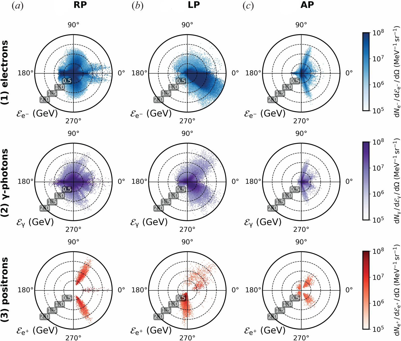
Figure 2. Polar energy spectrum diagrams of (1) electrons at ${\sim } 0.7 \ \mathrm {fs}$ and (2) $\gamma$
 -photons and (3) positrons generated in the time interval $-0.3 \ \mathrm {fs} \leqslant t \leqslant 0.7 \ \mathrm {fs}$
 , for (a) a RP laser, (b) a LP laser and (c) an AP laser. Animation for a larger time interval is provided in supplementary movie 1.
Within $t_b$ , high-amplitude oscillations of the electron momentum occur. At $t_c$
 , electron momentum oscillations become gradually less significant, with the electron spectrum eventually saturating. At this stage, the peak laser field is not completely reflected, but $E_x$
 starts forming a cavity beyond the over-dense electron front. Part of the laser field then reaches within the cavity, further expanding it. The initial times of this process witness instantaneous intensities an order of magnitude higher than the intensity expected on focus, due to interference of the laser fields after diffraction/reflection by the cavity walls. Although the intensity occurs only instantaneously, it was found to be ${\sim } 8.8 \times 10^{25} \ \mathrm {W}\ \mathrm {cm}^{{-2}}$
 in a region approximated by a sphere of ${\sim } 50 \ \mathrm {nm}$
 diameter, at $1.7 \ \mathrm {fs}$
 . At this stage, another electron population emerges, driven by the reflected field in the backward direction. In summary, during all stages of the laser–target interaction, electron populations at $0 ^{\circ }$
 , ${\sim } 60^{\circ }$
 and $180^{\circ }$
 are recorded.
So far, we have given a detailed explanation of the electron evolution under the influence of a RP $\lambda ^{3}$ laser. For a LP $\lambda ^{3}$
 laser, although the $E_x$
 still does exist, the lack of rotational symmetry does not allow the curled fields to take a toroidal form. Therefore, although a pre-plasma distribution is formed, it is extremely asymmetric along the laser oscillation direction. The thin over-dense electron pileup is also asymmetric. The asymmetry is due to the initial decay of the flat target, diverting the laser into a favourable direction. Asymmetric field interference does not allow the laser to form a conical cavity, but the random nature of the process forms a macroscopically rectangle-like cavity instead.
For the case of an AP $\lambda ^{3}$ laser the cavity formation is simpler. The absence of $E_x$
 means that the laser can be absorbed by the target in a manner similar to that of a weakly focused laser, suppressing the target deformation. The deformation takes the form of an over-dense electron pileup without pre-plasma. The pre-plasma created is also suppressed, in a region near the laser propagation axis. However, by the end of the simulation a cavity is eventually created, although by that time strong fields do not exist and $\kappa _\gamma$
 is limited, as discussed in § 3.2.
3.2 Evolution of $\gamma$-photons and positrons

At ultra-high laser intensities, $\gamma$ -photon and $\mathrm {e}^{-}$
 –$\mathrm {e}^{+}$
 pair generation plays an important role in the laser–target interaction. The non-trivial form of the $\lambda ^{3}$
 field reveals a strong dependency of $\gamma$
 -photon and $\mathrm {e}^{-}$
 –$\mathrm {e}^{+}$
 pair generation every quarter-period, in connection with the altered gradient/sign of the laser field, which in extension defines the electron motion as seen in § 3.1.
The $\gamma$ -photon generation can be visualised by a series of polar energy spectrum diagrams. An animation for various times is provided as supplementary material movie 1 available at https://doi.org/10.1017/S0022377821001318. However, since we are mainly interested in the evolution of $\gamma$
 -photon generation, it is more appropriate to consider the difference of every two subsequent polar diagrams, where our simulations output the data every $1 \ \mathrm {fs}$
 , a time interval similar to the quarter-period of $5/6 \ \mathrm {fs}$
 . The second row of figure 2 (see also the second row in supplementary movie 1) shows these diagrams for the three polarisations used, for a time interval of $-0.3 \ \mathrm {fs} \leqslant t \leqslant 0.7 \ \mathrm {fs}$
 . These diagrams have the benefit of not only showing at which angle $\gamma$
 -photons are generated, but also a negative value indicates $\gamma$
 -photon loss. In our simulations no $\gamma$
 -photons are allowed to escape the simulation and lack of $\gamma$
 -photons is attributed only to $\mathrm {e}^{-}$
 –$\mathrm {e}^{+}$
 pair formation. The corresponding plots for positrons are shown in the third row of figure 2. We must clarify that $\gamma$
 -photons and $\mathrm {e}^{-}$
 –$\mathrm {e}^{+}$
 pairs are not only formed in positive and negative polar diagram values, respectively, but a negative sign means that more $\gamma$
 -photons are lost to $\mathrm {e}^{-}$
 –$\mathrm {e}^{+}$
 pairs than are generated by the multi-photon Compton scattering process.
Let us consider a RP laser. Initially, up to $-2.3 \ \mathrm {fs}$ , only a small fraction of electrons obtain relativistic energies due to the low-amplitude periphery of the $\lambda ^{3}$
 field. These electrons then interact with the reflected relatively low-amplitude edge of the laser (Ridgers et al. Reference Ridgers, Brady, Duclous, Kirk, Bennett, Arber, Robinson and Bell2012) producing low-energy (${\sim } 0.1 \ \mathrm {GeV}$
 ) $\gamma$
 -photons. However, during the next femtosecond significantly more electrons acquire relativistic energies and in combination with the increased amplitude of the field as approaching the focal spot at ${\sim } 60^{\circ }$
 , directional $\gamma$
 -photons of ${\sim } 0.5 \ \mathrm {GeV}$
 appear at the same angle. In addition, another energetic electron population appears towards the laser propagation axis, producing another high-energy $\gamma$
 -photon population.
A similar process continues up to $-0.3 \ \mathrm {fs}$ , although electric fields are intensified giving $\gamma$
 -photons of ${\sim } 1 \ \mathrm {GeV}$
 . The newly generated $\gamma$
 -photons are still oriented purely at a ${\sim } 60 ^{\circ }$
 cone and also on the laser axis. It is no surprise that the $\gamma$
 -photon yield continues increasing until the laser pulse peak amplitude reaches the focal spot. What is a surprise is that the high-energy part of the $\gamma$
 -photon spectrum drops near that time. The overall increase in $\kappa _\gamma$
 is mostly due to an isotropic generation of moderate- to low-energy$\gamma$
 -photons.
In figure 2(c), one can observe the polar energy spectrum of positrons generated within $1 \ \mathrm {fs}$ time interval at ${\sim } 60^{\circ }$
 , corresponding to the conversion of high-energy $\gamma$
 -photons to $\mathrm {e}^{-}$
 –$\mathrm {e}^{+}$
 pairs. Strong $\mathrm {e}^{-}$
 –$\mathrm {e}^{+}$
 pair generation continues within the next 2 fs and then sharply decreases. This time interval is characterised by a region of negative values ($\gamma$
 -photon loss) in the high-energy part of the $\gamma$
 -photon energy spectra produced within a finite time, when plotted as a function of time. This plot (not shown) reveals the quarter-period behaviour of $\gamma$
 -photon generation as a superposition of several peaks. As the field amplitude drops, the $\gamma$
 -photon production rate also drops. One can approximate the $\gamma$
 -photon production rate as a steep Gaussian-like function up to the focus, followed by an exponential-like decay.
As mentioned in § 1, a LP laser results in a higher peak intensity compared to a RP laser of the same power. Although the lack of symmetry results in a weaker coupling of the laser energy to the target electrons, the higher intensity on focus results in a slight enhancement of the high-energy part of the $\gamma$ -photon energy spectrum for the LP laser case. However, at energies lower than ${\sim } 0.37 \ \mathrm {GeV}$
 the amplitude of the $\gamma$
 -photon energy spectrum is higher for the RP laser case. Consider that for the RP laser, $\gamma$
 -photons with energy ${<\sim }0.37\ \mathrm {GeV}$
 contain ${\sim } 90\,\%$
 of the $\gamma$
 -photon energy. Therefore, although the LP laser results in higher cut-off energies, it results in $\kappa _\gamma$
 of ${\sim } 40\,\%$
 , compared with ${\sim } 47\,\%$
 for a RP laser. For the AP laser, although strong fields do exist, the Lorentz factor of electrons is significantly lower than for the other two polarisation cases. Furthermore, no significant pre-plasma is formed in the laser field reflection region. As a result, $\kappa _\gamma$
 of only ${\sim } 20\,\%$
 occurs.
The positron spectra for LP and RP lasers overlap, apart from in the very high and very low parts of the spectra, where the positrons obtain $\kappa _{e+}$ ${\sim } 7\,\%$
 and ${\sim } 9\,\%$
 by the end of the simulation. However, this energy is not purely a result of $\gamma$
 -photon energy conversion to $\mathrm {e}^{-}$
 –$\mathrm {e}^{+}$
 pairs, but it is also a result of acceleration/deceleration of those positrons by the laser field, in the same manner as electrons (Ridgers et al. Reference Ridgers, Brady, Duclous, Kirk, Bennett, Arber, Robinson and Bell2012). One index that can directly compare two interactions is the number of positrons generated, regardless of their energy, where for a RP laser and a LP laser we obtain ${\sim } 5.7 \times 10^{11}$
 and ${\sim } 4 \times 10^{11}$
 positrons, respectively. In comparison, the AP laser results in $\kappa _{e+}$
 ${\sim }3\,\%$
 , but generation of only ${\sim } 1.9 \times 10^{11}$
 positrons. The imbalance of $\kappa _{e+}$
 to number of positrons for the various laser polarisation modes verifies that positrons are strongly affected by the laser field after their generation.
In addition, our simulations record local positron number densities as high as ${\sim } 3 \times 10^{26}\ \mathrm {cm}^{{-3}}$ , approximately two orders of magnitude higher than the titanium target electron number density, emphasising the collective effect of $\mathrm {e}^{-}$
 –$\mathrm {e}^{+}$
 pairs in the laser–targetinteraction. By assuming that the $\mathrm {e}^{-}$
 –$\mathrm {e}^{+}$
 pairs are contained in a uniform density sphere of diameter equal to that of the $\lambda ^{3}$
 laser, they correspond to an average number density of ${\sim } 10^{25} \ \mathrm {cm}^{{-3}}$
 , still an order of magnitude higher than the target electron number density.
3.3 The $\gamma$-ray flash

As mentioned in Hadjisolomou et al. (Reference Hadjisolomou, Jeong, Valenta, Korn and Bulanov2021), the $\gamma$ -photons generated during the interaction of a RP $\lambda ^{3}$
 laser with a foil appear in the form of a spherically expanding shell. The $\gamma$
 -photon energy density of this shell is not uniform since more energetic $\gamma$
 -photons are at $0^{\circ }$
 , $180^{\circ }$
 and ${\sim }60^{\circ }$
 . Computational constraints limit the $\gamma$
 -photon shell expansion within a cube of $\pm 5.12 \ \mathrm {\mu }\mathrm {m}$
 edges. In the EPOCH code, if a $\gamma$
 -photon is not lost to an $\mathrm {e}^{-}$
 –$\mathrm {e}^{+}$
 pair, then it propagates ballistically. Therefore, the $\gamma$
 -photon located at position $(x_{i,1},y_{i,1},z_{i,1})$
 can propagate a distance $\mathcal {D}$
 to a new position $(x_{i,2},y_{i,2},z_{i,2})$
 (where the subscript $i$
 denotes the corresponding $\gamma$
 -photon of energy $\mathcal {E}_i$
 ):
):


which corresponds to a new distance $r_i$ from the axis origin.
The ballistic $\gamma$ -photon expansion for a $\mathcal {D}$
 of $15.36 \ \mathrm {\mu } \mathrm {m}$
 reveals that the $\gamma$
 -photon population at $60^{\circ }$
 rapidly decreases geometrically. However, the $\gamma$
 -photon populations at $0^{\circ }$
 and $180^{\circ }$
 due to their small solid angle are preserved, as shown in figure 3(a). The spherically expanding $\gamma$
 -ray flash at large distances is considered as originating from a virtual point source, although as seen in § 3.2 the $\gamma$
 -photons are not generated instantaneously.

Figure 3. The $\gamma$ -photon radiant intensity for (a) a RP laser, (b) a LP laser and (c) an AP laser, $64\ \mathrm {fs}$
 after the start of the simulation. Electron number density cross-section at $x = 0.5 \ \mathrm {\mu }\mathrm {m}$
 for (d) a RP laser, (e) a LP laser and (f ) an AP laser, at the end of the simulation.
As mentioned earlier for a RP laser, $\gamma$ -photons obtain ${\sim } 47\,\%$
 of the ${\sim } 280 \ \mathrm {J}$
 laser energy, or in other words, the $\gamma$
 -ray flash energy is ${\sim } 130 \ \mathrm {J}$
 . To calculate the mean location of the $\gamma$
 -ray flash, $\mu$
 , we calculate the first-order moment as

which for the RP laser case gives $\mu {\sim } 18.5 \ \mathrm {\mu }\mathrm {m}$ .
.
The second-order moment gives the position variance, $\sigma ^{2}$ , of the $\gamma$
 -ray flash as

while the square root of the variance gives the standard deviation, which in turn gives the temporal FWHM of the $\gamma$ -ray flash. For a RP laser the $\gamma$
 -ray flash has a FWHM duration of ${\sim } 4.2 \ \mathrm {fs}$
 resulting in a $\gamma$
 -ray flash of ${\sim } 31 \ \mathrm {PW}$
 .
.
For a LP laser and an AP laser the $\gamma$ -ray flash power is ${\sim } 28$
 and ${\sim } 13 \ \mathrm {PW}$
 , respectively. The AP laser results in high-energy $\gamma$
 -photons emitted mainly at ${\sim } 60^{\circ }$
 , while the dominant low-energy $\gamma$
 -photons are emitted isotropically, as shown in figure 3(c). The LP laser case results in two detached $\gamma$
 -photon fronts delayed by a half-period at ${\sim }\pm 45^{\circ }$
 and with higher $\gamma$
 -photon energy density on the plane defined by the laser field oscillation. At large distances, these fronts merge, and therefore expand as thin rings, as seen in figure 3(b). The energy, mean position, position variance, duration and power of the $\gamma$
 -ray flash for RP, LP and AP lasers are summarised in table 2.
Table 2. Energy, mean position, position variance, duration and power of the $\gamma$ -ray flash for RP, LP and AP lasers.
The electron number density for the RP laser case forms radially symmetric regular modulations inside the target cavity (figure 3d). The effect of those modulations is reflected in the $\gamma$ -photon radiant intensity distribution, as shown in figure 3(a). For the LP laser case, although electron modulations are formed, they are symmetric only with respect to the laser oscillation direction (figure 3e). Therefore, radial $\gamma$
 -photon modulations are not observed (figure 3b) and any $\gamma$
 -photon modulation is hidden by the macroscopic $\gamma$
 -photon distribution. Similar patterns have been observed for a LP laser in both two-dimensional (Nakamura et al. Reference Nakamura, Koga, Esirkepov, Kando, Korn and Bulanov2012) and three-dimensional (Stark, Toncian & Arefiev Reference Stark, Toncian and Arefiev2016; Wang et al. Reference Wang, Ribeyre, Gong, Jansen, d'Humières, Stutman, Toncian and Arefiev2020a) simulations. For the AP laser case, radial electron modulations are formed, but with outwards directionality. Furthermore, they are shielded inthe field region by an over-dense electron ring distribution (figure 3f ). As a result, no obvious $\gamma$
 -photon modulations are observed.
3.4 Mapping the energy conversion efficiency
In the current subsection we present the results of our multi-parametric study for an ${\sim } 80 \ \mathrm {PW}$ laser (RP, LP and AP laser cases) with $\kappa _\gamma$
 , $\kappa _{e+}$
 , laser to electron energy conversion efficiency $\kappa _{e-}$
 and laser to ion energy conversion efficiency $\kappa _{i+}$
 . The variable parameters include the target thickness and electron number density, for which the inversely proportional relation is mentioned in § 1. The results are presented in the form of ternary plots (West Reference West1982) accompanied by radar charts.
Unavoidably, interaction of a laser field with matter results in transformation of some laser energy to particle energy. The dependency of $\kappa$ on the electron number density and target thickness can be seen in figure 4, where the direction of the grey arrow in the figure indicates increasing thickness. For both RP and LP lasers, increased laser to all particles energy conversion efficiency, $\kappa _{{\rm tot}} = \kappa _\gamma + \kappa _{e+} + \kappa _{e-} + \kappa _{i+}$
 , occurs for thicker and denser targets, ${\sim } 80\,\%$
 and ${\sim } 85\,\%$
 for RP and LP lasers, respectively. For thinner and low-density targets, the particles obtain only ${\sim } 40\,\%$
 of the laser energy for both RP and LP lasers (within the parameter ranges examined). For an AP laser for thin and low-density targets, $\kappa _{{\rm tot}}$
 is approximately half compared to that for RP and LP lasers. For an AP laser (in contrast to the continuously increasing $\kappa _{{\rm tot}}$
 behaviour for RP and LP lasers) beyond of an optimal thickness–density combination, $\kappa _{{\rm tot}}$
 starts decreasing for thicker and denser targets (maximum is ${\sim } 60\,\%$
 ), in connection with the inefficient target cavity formation (see § 3.1) and increasing laser back-reflection as electron number density increases.

Figure 4. (Left) Ternary plots of $\kappa _\gamma$ , $\kappa _{ch}$
 and $\kappa _{{\rm EM}}$
 for samples with varying electron number density and target thickness. The grey arrow points towards increasing foil thickness. (Right) Selected radar charts (solid line for $2 \ \mathrm {\mu }\mathrm {m}$
 and dotted line for $0.2 \ \mathrm {\mu }\mathrm {m}$
 thick foil; red for $2\ \times 10^{23}\ \mathrm {cm}^{{-3}}$
 , blue for $1 \times 10^{24} \ \mathrm {cm}^{{-3}}$
 and green for $5 \times 10^{24}\ \mathrm {cm}^{{-3}}$
 electron number density) of $\kappa _\gamma$
 , $\kappa _{e+}$
 , $\kappa _{e-}$
 , $\kappa _{i+}$
 and $\kappa _{{\rm EM}}$
 . (a) A RP laser, (b) a LP laser and (c) an AP laser.
In general, ions, being heavier than electrons, do not produce high-energy $\gamma$ -photons. However, they indirectly affect the $\gamma$
 -photon spectrum. Their contribution arises from the amount of the laser energy transferred to them, consequently reducing electron energy and therefore what can otherwise be converted to $\gamma$
 -photons. For all polarisation cases, $\kappa _{i+}$
 increases with increasing electron number density up to an optimum value and then decreases for thicker targets (Esirkepov et al. Reference Esirkepov, Borghesi, Bulanov, Mourou and Tajima2004; Klimo et al. Reference Klimo, Psikal, Limpouch and Tikhonchuk2008; Robinson et al. Reference Robinson, Zepf, Kar, Evans and Bellei2008; Bulanov et al. Reference Bulanov, Esarey, Schroeder, Bulanov, Esirkepov, Kando, Pegoraro and Leemans2016). Therefore, although thin targets can be dense enough to convert a large fraction of laser energy to particle energy, that energy goes primarily to ions. For thick targets, although more laser energy is converted to particle energy by increasing the electron number density, since $\kappa _{i+}$
 also increases, it competes with what is converted to $\kappa _\gamma$
 , $\kappa _{e-}$
 and $\kappa _{e+}$
 , forbidding the optimum of those particles to exist at extremely high electron number density values. For optimal thickness and density combinations, for all three polarisations, $\kappa _{i+}$
 reaches ${\sim } 25\,\%$
 .
.
Where $\kappa _{i+}$ is not efficient, $\kappa _{e-}$
 and $\kappa _{e+}$
 cover the imbalance. For all laser polarisation modes, if the electron number density is extremely low then the laser pulse propagates through the target. Alternatively, if the target is thick enough then most of the laser energy is absorbed, resulting in enhanced $\kappa _{e-}$
 . For RP and LP lasers, $\kappa _{e-}$
 is ${\sim } 20\,\%$
 , while for an AP laser it is ${\sim } 15\,\%$
 at optimum target parameters. Some slow $\kappa _{e-}$
 increase for extremely high electron number densities is due to less accurate resolution of the relativistically corrected skin depth, although the increase is insignificantly small to alter the conclusion of the other particle species at that density. For RP and LP lasers, a high $\kappa _{e-}$
 also occurs for thin targets in regions where $\kappa _{i+}$
 is not efficient, due to electron capture by the laser field (Wang et al. Reference Wang, Ho, Yuan, Kong, Cao, Sessler, Esarey and Nishida2001).
Although for an ${\sim } 80 \ \mathrm {PW}$ laser a significant number of $\mathrm {e}^{-}$
 –$\mathrm {e}^{+}$
 pairs are generated, their number is still relatively low (approximately 50 times lower) compared with the number of electrons contained in the target prior to the laser–foil interaction. However, those $\mathrm {e}^{-}$
 –$\mathrm {e}^{+}$
 pairs are generated in regions of ultra-intense fields, and therefore are more strongly heated compared with the electrons in the periphery of the target cavity. The $\mathrm {e}^{-}$
 –$\mathrm {e}^{+}$
 pairs more probably originate from $\gamma$
 -photons of higher energy. Therefore, $\kappa _{e+}$
 is a combination of the energy they obtain from the Breit–Wheeler process and the energy due to acceleration/deceleration from the laser field. The thickness–density contour of $\kappa _{e+}$
 has partial topological similarities to that of $\kappa _{i+}$
 , meaning that positrons are affected by the laser field in a manner similar to that of ions. The $\kappa _{e+}$
 for RP and LP lasers reaches ${\sim } 10\,\%$
 , while it is approximately half for an AP laser. In contrast to electrons, positrons cannot obtain high $\kappa _{e+}$
 for under-dense thick targets because of their low number generated at these parameter values.
By combining the laser to all charged particles energy conversion efficiency, $\kappa _{ch} = \kappa _{e+} + \kappa _{e-} + \kappa _{i+}$ , we conclude a maximum value of ${\sim } 45\,\%$
 that slowly increases with increasing target thickness, as shown in figure 4. On the other hand, the figure exhibits a steep increase of $\kappa _\gamma$
 for increasing target thickness, where the maximum values are mentioned in § 3.2. For a LP laser, the topology of the $\kappa _\gamma$
 thickness–density contour is in agreement with that of $\kappa _{{\rm tot}}$
 , being maximised for thick and dense targets. On the other hand, for the RP laser, although the $\kappa _\gamma$
 thickness–density contour resembles that of the LP laser for most thickness–density combinations, a maximum is observed at an electron number density of $1.2 \times 10^{24} \ \mathrm {cm}^{{-3}}$
 . This local maximum is due to the different rate of energy transfer to ions, where for a RP laser it is lower at that electron number density. In addition, $\kappa _{{\rm tot}}$
 is slightly higher for the RP laser at thicker and denser targets, further enhancing the local maxima of $\kappa _\gamma$
 . For an AP laser, $\kappa _\gamma$
 has an optimal electron number density at $5 \times 10^{23} \ \mathrm {cm}^{{-3}}$
 since the lack of $E_x$
 requires a target of lower electron number density for efficient laser–target coupling. For more accurate $\kappa$
 for each particle species at the extreme thickness–density values, see the right-hand side of figure 4.
3.5 Dependency on the laser power
As we have shown for an ${\sim } 80 \ \mathrm {PW}$ RP laser, $\kappa _\gamma$
 is ${\sim } 47\,\%$
 for targets thicker than $2 \ \mathrm {\mu }\mathrm {m}$
 and an electron number density of $1.2 \times 10^{24} \ \mathrm {cm}^{{-3}}$
 . A consequent question arises as to why the choice of ${\sim } 80 \ \mathrm {PW}$
 is made and what is the effect of altering the laser power. To address that topic, the simulations for a RP laser were extended in the power range of $1\ \mathrm {PW} \leqslant P \leqslant 300 \ \mathrm {PW}$
 , where the electron number density was varying in the range $10^{23} \ \mathrm {cm}^{{-3}} \leqslant n_e \leqslant 10^{24} \ \mathrm {cm}^{{-3}}$
 . As per the results of § 3.4, $\kappa _\gamma$
 varies insignificantly on decreasing the electron number density from $1.2 \times 10^{24}\ \mathrm {cm}^{{-3}}$
 to $10^{24} \ \mathrm {cm}^{{-3}}$
 .
.
Let us consider the case where the electron number density is fixed at $10^{24} \ \mathrm {cm}^{{-3}}$ and the laser power varies. The value of $\kappa$
 of each species is shown in figure 5, where $a_0 \approx 307$
 for $1 \ \mathrm {PW}$
 , while $a_0 \approx 5318$
 for $300 \ \mathrm {PW}$
 . Plots of $\kappa _\gamma$
 , $\kappa _{e+}$
 , $\kappa _{e-}$
 and $\kappa _{i+}$
 are shown as black, red, blue and green continuous lines, respectively, while the percentage of the laser energy remaining as electromagnetic energy, $\kappa _{{\rm EM}}$
 , is shown by the purple continuous line.
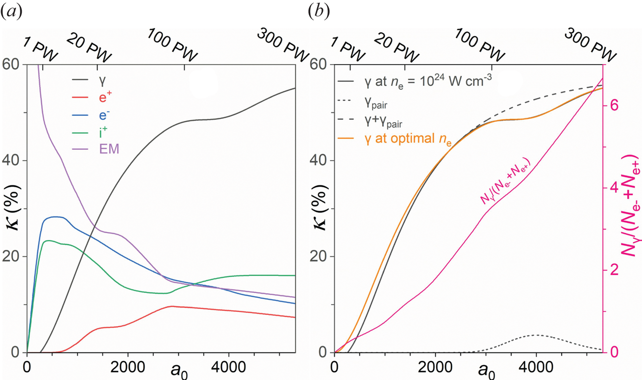
Figure 5. Values of (a) $\kappa _\gamma$ (black line), $\kappa _{e+}$
 (red line), $\kappa _{e-}$
 (blue line), $\kappa _{i+}$
 (green line) and $\kappa _{{\rm EM}}$
 (purple line) as a function of $a_0$
 for a RP $\lambda ^{3}$
 laser and an electron number density of $10^{23} \text {--} 10^{24} \ \mathrm {cm}^{{-3}}$
 . (b, left-hand axis) Plot of $\kappa _\gamma$
 fitted with (3.6) for an electron number density of $10^{23} \text {--} 10^{24} \ \mathrm {cm}^{{-3}}$
 (black solid line) and at the optimum electron number density at each power (orange line). The fitted curve is the difference of a ‘Logistic’ function (long-dashed black line) and a ‘LogNormal’ function (short-dashed black line), as defined in the text. (b, right-hand axis) The ratio of the $\gamma$
 -photon number over the sum of electron and positron numbers as a function of $a_0$
 for an electron number density of $10^{23} \text {--} 10^{24} \ \mathrm {cm}^{{-3}}$
 .
.
From the purple line in figure 5 one can observe that at low laser power the laser cannot be efficiently absorbed by the target and it is mostly reflected, since at low power the skin depth does not have significant relativistic increase. However, by increasing the laser power to $20 \ \mathrm {PW}$ , corresponding to $a_0 \sim 1400$
 , ${\sim } 75\,\%$
 of the laser energy is absorbed by the target. On further increasing the power up to $300 \ \mathrm {PW}$
 ,the percentage of laser energy absorbed increases, although with a lower rate as power increases and eventually saturating at ${\sim } 10\,\%$
 .
.
At ${\sim } 20 \ \mathrm {PW}$ , $\kappa _\gamma$
 , $\kappa _{e-}$
 and $\kappa _{i+}$
 become equally important. At $P \lessapprox 5 \ \mathrm {PW}$
 , most of the laser energy is transferred to electrons and ions, with $\gamma$
 -photons and positrons obtaining an insignificantly low laser energy fraction. However, the picture reverses for $P \gtrapprox 20 \ \mathrm {PW}$
 , where $\kappa _{i+}$
 saturates at ${\sim } 15\,\%$
 . The value of $\kappa _{e-}$
 also exhibits a plateau region at $1 \ \mathrm {PW} \lessapprox P \lessapprox 5 \ \mathrm {PW}$
 , after which $\kappa _{e-}$
 continuously decreases for increasing laser power and eventually saturating at ${\sim } 10\,\%$
 . The value of $\kappa _{e+}$
 continuously increases for laser power up to ${\sim } 80 \ \mathrm {PW}$
 , where after obtaining a maximum value of ${\sim } 9\,\%$
 it decreases to ${\sim } 5\,\%$
 for higher power values.
The trend of $\kappa _\gamma$ in figure 5 changes at a power of ${\sim } 80 \ \mathrm {PW}$
 . Since $\kappa _{e+}$
 , $\kappa _{e-}$
 and $\kappa _{i+}$
 all saturate for increasing power, then $\kappa _\gamma$
 unavoidably also saturates, where the sum of $\kappa _{e+}$
 , $\kappa _{e-}$
 and $\kappa _{i+}$
 suggests a $\kappa _\gamma$
 saturation at ${\sim } 60\,\%$
 . Therefore, we treat the $\kappa _\gamma$
 function as the difference of a ‘Logistic’ and a ‘LogNormal’ function, given respectively by the left- and right-hand parts of the following equation:

The Logistic function is a saturating function representing $\gamma$ -photon generation. The LogNormal function is an asymmetric peak function which is chosen for $\gamma$
 -photon loss representation due to $\mathrm {e}^{-}$
 –$\mathrm {e}^{+}$
 pair generation, since its asymmetric behaviour allows fitting without prior knowledge of the physical loss (or gain) behaviour. Fitting of (3.6) to $\kappa _\gamma$
 as shown in figure 5(b) gives $A_1 \approx -1.75$
 , $A_2 \approx 59.8$
 , $p \approx 2.05$
 , $x_0 \approx 1463$
 , $A_3 \approx 2213$
 , $w \approx -0.151$
 and $x_c \approx 4088$
 .
.
The Logistic function (black dashed line in figure 5b) explains the expected $\kappa _\gamma$ saturation for an increasing laser power. The parameter $A_2$
 suggests $\kappa _\gamma$
 saturation at ${\sim } 59.8\,\%$
 , while the parameter $A_1$
 suggests that at an electron number density of $10^{24} \ \mathrm {cm}^{{-3}}$
 no $\gamma$
 -photons can be produced for a laser power of ${\sim } 0.7 \ \mathrm {PW}$
 . The LogNormal function (black dotted line in figure 5b), having a negative sign, suggests that a $\gamma$
 -photon population is lost to $\mathrm {e}^{-}$
 –$\mathrm {e}^{+}$
 pairs, where their contribution becomes most significant for ${\sim } 177 \ \mathrm {PW}$
 as suggested by the parameter $x_c$
 .
.
By repeating the analysis described above for electron number densities in the range $10^{23} \ \mathrm {cm}^{{-3}} \leqslant n_e \leqslant 10^{24} \ \mathrm {cm}^{{-3}}$ we find the optimal electron density value at each power for maximising $\kappa _\gamma$
 , plotted by the orange line in figure 5(b). The trend suggests that $1 \ \mathrm {PW}$
 is sufficient for $\kappa _\gamma$
 of ${\sim } 3\,\%$
 . The density–power contour suggests that $\kappa _\gamma$
 is strongly dependent on the electron number density at low laser power, optimal at $2 \times 10^{23} \ \mathrm {cm}^{{-3}}$
 for a $1 \ \mathrm {PW}$
 laser. By increasing the laser power, denser targets are required to give the peak $\kappa _\gamma$
 , although the density dependency becomes less prominent as power increases.
The pink line on the right-hand side of figure 5(b) shows the ratio of $\gamma$ -photon number produced to the sum of electron and positron numbers as a function of $a_0$
 . The line exhibits an approximately linearly increasing trend, suggesting that at higher laser powers each electron/positron can emit $\gamma$
 -photons several times by the end of the simulation. For an ${\sim } 80 \ \mathrm {PW}$
 laser, each electron/positron emits $\gamma$
 -photons approximately three times.
4 Interaction of $\gamma$-ray flash with high-$Z$ target


In order to examine the effect of the $\gamma$ -ray flash described in § 3.3 on a secondary, high-$Z$
 target, we perform MC simulations using the FLUKA code (Battistoni et al. Reference Battistoni, Boehlen, Cerutti, Chin, Esposito, Fassò, Ferrari, Lechner, Empl and Mairani2015; Böhlen et al. Reference Böhlen, Cerutti, Chin, Fassò, Ferrari, Ortega, Mairani, Sala, Smirnov and Vlachoudis2014) and its graphical interface FLAIR (Vlachoudis Reference Vlachoudis2009). In addition to $\gamma$
 -photons, the effects of the charged PIC-produced particles on the secondary target are also investigated. The PIC output particles (type, position, momentum and weight) are imported to FLUKA as primary particles. The secondary target is modelled as a $10\ \mathrm {mm}$
 thick disk of $100\ \mathrm {mm}$
 in diameter and it is located at $0.1\ \mathrm {mm}$
 from the focal spot coordinates. The large acceptance angle covered by the secondary target allows one to intercept almost all PIC-generated particles in the forward direction. Natural lead, Pb, is chosen as material for the disk because of its high cross-section for pair production and photonuclear interactions for energies considered. For the simulations, the FLUKA PRECISIO defaults are used. Additionally, the electromagnetic transport thresholds are set at $0.1 \ \mathrm {MeV}$
 , the photonuclear and electronuclear interactions are enabled, as well as the evaporation of heavy fragments and nuclear coalescence.
Figure 6 shows the PIC-generated positrons moving in the forward direction, exhibiting a rather flat spectrum with a temperature of ${\sim } 0.4 \ \mathrm {GeV}$ . The figure overplots the spectra of positrons escaping the secondary target in the forward direction, obtained from the MC simulations, integrated (black dashed line) and separated per primary particle species (solid lines), namely $\gamma$
 -photons, electrons, positrons and titanium ions. From figure 6 it is seen that the largest number of positrons (${\sim } 81.4\,\%$
 ) is produced by $\gamma$
 -photons and that the most energetic positrons are those directly created in the PIC simulations.

Figure 6. For each $\lambda ^{3}$ pulse, the energy spectrum of the PIC positrons moving in the forward direction (red dashed), along with the positron spectra from the MC simulations in total (black dashed line) and separated per producing species ($\gamma$
 -photons (black), electrons (blue), positrons (red) and titanium ions (green)).
Positrons produced by PIC $\gamma$ -photons and electrons have a temperature of ${\sim } 0.1 \ \mathrm {GeV}$
 . The positron population exhibits two temperatures, the first of ${\sim } 0.1 \ \mathrm {GeV}$
 corresponding to those generated in the lead target, and the second at higher temperature corresponding to PIC-generated positrons. The low-temperature positrons are generated via $\mathrm {e}^{-}$
 –$\mathrm {e}^{+}$
 pair production from Bremsstrahlung $\gamma$
 -photons. The positron spectra after the secondary target areshifted towards lower energy with respect to the PIC-produced positrons, while their total number is increased by approximately an order of magnitude.
Monte Carlo simulations also allow one to estimate the number of stable and unstable nuclides generated in the lead target. Figure 7 shows achart of the produced nuclides focused around the lead position and separated per PIC particle species. Stable nuclides are highlighted with a box. Most of the residual nuclides are produced through photonuclear interactions, either directly by primary (PIC) $\gamma$ -photons or indirectly by secondary (Bremsstrahlung from fast electrons/positrons) $\gamma$
 -photons. In our $\gamma$
 -photon energy region of interest, the giant dipole resonance photonuclear process dominates since it has the highest integrated cross-section, peaking at ${\sim } 13.6 \ \mathrm {MeV}$
 $\gamma$
 -photons. Apart from photonuclear interactions, residual nuclides can be also produced by nucleus–nucleus interactions and/or electronuclear interactions.
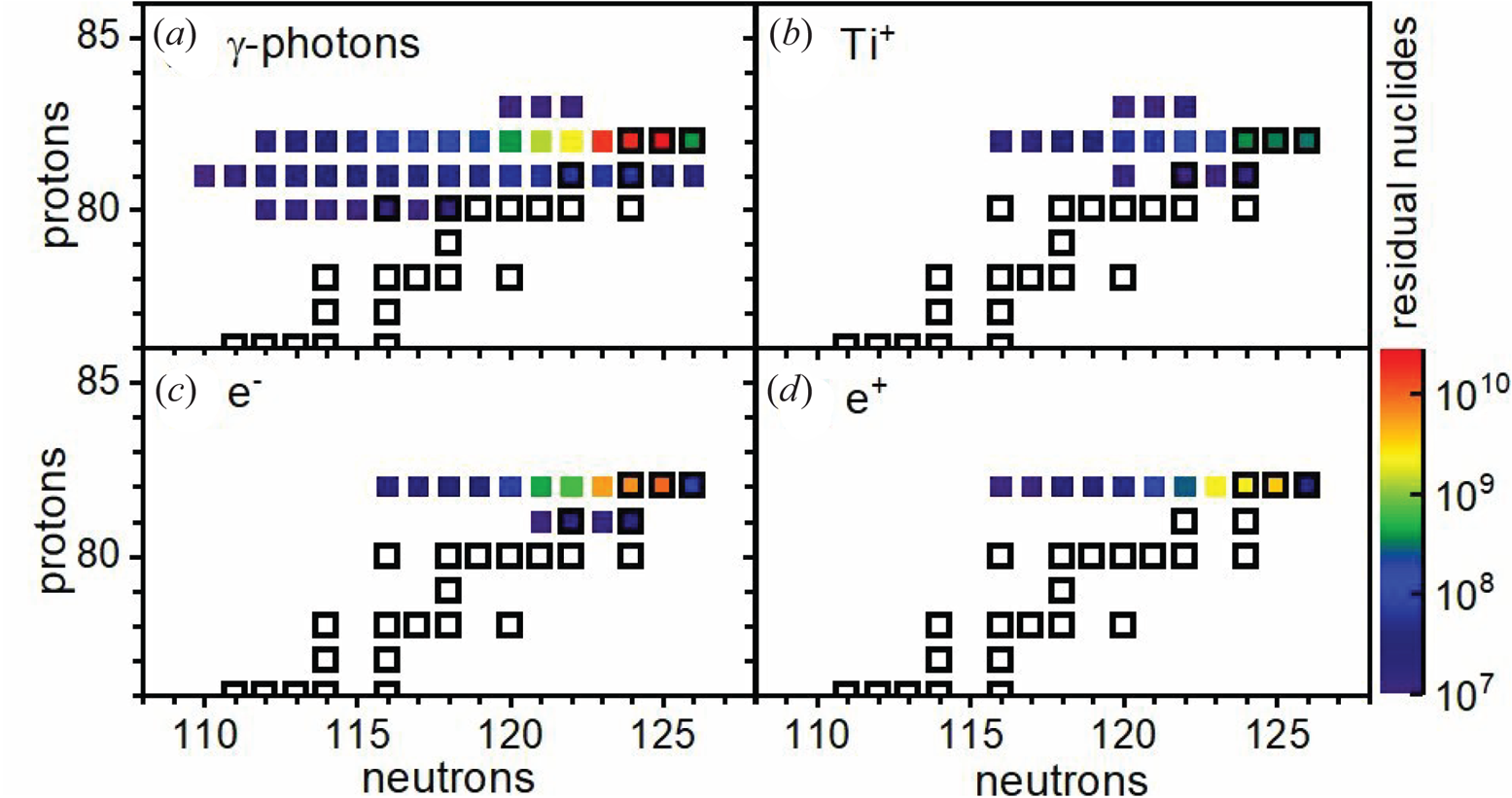
Figure 7. Chart of residual nuclides obtained from MC simulation per $\lambda ^{3}$ pulse and separated per PIC particle species. Stable nuclides are highlighted with a box.
One of the most abundant generated lead isotopes is ${}^{203}_{82}{\rm Pb}$ , where ${\sim } 10^{9}$
 nuclides are produced with a half-life of ${\sim } 52 \ \mathrm {h}$
 . Its direct decay to ${}^{203}_{81}{\rm Tl}$
 (stable) is through electron capture and it does not emit any hadrons. In addition, photons of ${\sim } 279.2 \ \mathrm {keV}$
 are emitted which are particularly suitable for medical imaging (Azzam, Said & Al-abyad Reference Azzam, Said and Al-abyad2014). The second most abundant isotope produced is thallium, with ${}^{201}_{81}{\rm Tl}$
 (${\sim } 10^{8}$
 nuclides) historically beingused extensively for nuclear medicine (Tadamura et al. Reference Tadamura, Kudoh, Motooka, Inubushi, Shirakawa, Hattori, Okada, Matsuda, Koshiji and Nishimura1999) due to its decay to ${}^{201}_{80}{\rm Hg}$
 (stable) through electron capture with a half-life of ${\sim } 73 \ \mathrm {h}$
 .
.
5 Summary and conclusions
In this work we study highly efficient $\gamma$ -photon generation through an ultra-intense laser and solid target interaction. We employ the $\lambda ^{3}$
 regime, where a single-cycle laser pulse (${\sim } 80 \ \mathrm {PW}$
 ) is focused to a sphere ${\sim } \lambda /2$
 in diameter. The benefit of the $\lambda ^{3}$
 regime is that it provides the highest intensity achievable at a given laser power, at the expense of the least energy. In this paper we study the interaction of a $\lambda ^{3}$
 laser with matter in the quantum electrodynamics regime, where copious numbers of $\gamma$
 -photons and $\mathrm {e}^{-}$
 –$\mathrm {e}^{+}$
 pairs are generated. The quantum electrodynamics processes are studied by use of the three-dimensional EPOCH PIC code. The $\lambda ^{3}$
 laser fields are imported into EPOCH after being calculated independently through our developed code.
Our work examines the laser–target interaction for RP, LP and AP lasers. A multi-parametric study is presented, where the variables include the target thickness and electron number density. It is found that the optimal $\kappa _\gamma$ reaches ${\sim } 47\,\%$
 and it occurs for a RP laser at a target thickness of $2 \ \mathrm {\mu } \mathrm {m}$
 and an electron number density of $1.2 \times 10^{24}\ \mathrm {cm}^{{-3}}$
 . For the same target parameters, the LP and AP lasers result in $\kappa _\gamma$
 of ${\sim } 40\,\%$
 and ${\sim } 20\,\%$
 , respectively. For the optimal target variables, the LP laser gives $\kappa _\gamma$
 of ${\sim } 42\,\%$
 , while the AP laser gives $\kappa _\gamma$
 of ${\sim } 29\,\%$
 .
.
The significantly higher $\kappa _\gamma$ for the RP laser is due to the dominance of the longitudinal, $E_x$
 , field that increases the coupling of the laser to the target. For the LP laser $E_x$
 is smaller, while for the AP laser it is absent. The $E_x$
 field assists in the formation of a target cavity, where the cavity propagation performs a different propagation depending on the laser polarisation mode. Interference of the reflected/diffracted laser field inside the cavity results in an instantaneous intensity as high as ${\sim } 8.8 \times 10^{25} \ \mathrm {W}\ \mathrm {cm}^{{-2}}$
 , approximately one order of magnitude higher than the intensity expected on focus.
The directionality of electrons at several instances is identified, resulting in several high-energy electron groups directed at ${\sim } 0^{\circ }$ , ${\sim } 180^{\circ }$
 and ${\sim }60^{\circ }$
 for a RP laser. Those electrons are connected to the $\gamma$
 -photon directionality, being at the same angles. The ultra-high intensities employed result in not only prolific $\gamma$
 -photon generation but unavoidably also $\mathrm {e}^{-}$
 –$\mathrm {e}^{+}$
 pair generation through the multi-photon Breit–Wheeler process. The generation positions of $\mathrm {e}^{-}$
 –$\mathrm {e}^{+}$
 pairs is identified to overlap the regions of high-energy $\gamma$
 -photons.
At a time of ${\sim } \lambda /(2 c)$ after the peak of the laser pulse reaches the focal spot, the $\gamma$
 -photons expand radially in a ballistic fashion without significant losses to $\mathrm {e}^{-}$
 –$\mathrm {e}^{+}$
 pairs. The $\gamma$
 -photons expand within a spherical shell where the FWHM of their energy density is approximately equal to the laser wavelength, similar to the laser–foil interaction time. The expanding spherical shell for the RP, LP and AP lasers results in a $\gamma$
 -ray flash of ${\sim } 31$
 , ${\sim } 28$
 and ${\sim } 13 \ \mathrm {PW}$
 , respectively. Although a preferred directionality exists for the $\gamma$
 -photons, the radiant intensity of the population at ${\sim } 60^{\circ }$
 is less significant due to its large solid angle, in contrast to $\gamma$
 -photons at ${\sim } 0^{\circ }$
 and ${\sim } 180^{\circ }$
 .
.
Our analysis is also extended to varying the laser power in the range $1 \ \mathrm {PW} \leqslant P \leqslant 300 \ \mathrm {PW}$ . We demonstrate that $\kappa _\gamma$
 sharply increases up to ${\sim } 80 \ \mathrm {PW}$
 , while $\gamma$
 -photons become the dominant species above ${\sim } 20 \ \mathrm {PW}$
 . For low laser powers, there is a strong dependency of $\kappa _\gamma$
 on the electron number density, where the optimal electron number density increases approximately linearly with $a_0$
 . For higher power values this dependency becomes less important. When increasing the laser power then $\kappa _\gamma$
 increases, saturating at ${\sim } 60\,\%$
 . A $\kappa _\gamma$
 discontinuity exists centred at ${\sim } 177\ \mathrm {PW}$
 , attributed to the $\gamma$
 -photon conversion to $\mathrm {e}^{-}$
 –$\mathrm {e}^{+}$
 pairs, while as power further increases the $\gamma$
 -photon reduction is compensated by further $\gamma$
 -photon emission by positrons, in the same manner as by electrons. In addition, as laser power increases then the number of $\gamma$
 -photons emitted from each electron/positron also increases in an approximately linear fashion with $a_0$
 .
.
Finally, for the RP laser, the interaction of the PIC-generated particles interacting with a high-$Z$ target is studied by MC simulations. The spectra of each particle species escaping the secondary target are obtained. The PIC spectra are substantially altered by the interaction with the high-$Z$
 target. The $\gamma$
 -ray flash interaction with the secondary target also results in significant production of radioactive nuclides, whose yields are estimated. Hence, the coupling of PIC and MC simulations provides a powerful tool for further investigating the interaction of lasers with matter.
Supplementary movie
Supplementary movie is available at https://doi.org/10.1017/S0022377821001318.
Acknowledgements
The authors would like to acknowledge useful communication with Dr D. Khikhlukha and K. Lezhnin. This work is supported by the projects High Field Initiative (CZ.02.1.01/0.0/0.0/15$\_$ 003/0000449) from the European Regional Development Fund and ‘e-INFRA CZ’ (ID:90140) from the Ministry of Education, Youth and Sports of the Czech Republic. C.P.R. would like to acknowledge funding from EPSRC, grant no. EP/V049461/1. The EPOCH code is in part funded by UK EPSRC grants EP/G054950/1, EP/G056803/1, EP/G055165/1 and EP/M022463/1.
Editor Luís O. Silva thanks the referees for their advice in evaluating this article.
Declaration of interests
The authors report no conflict of interest.
Appendix A
This appendix gives the imaginary part of the integrands used for the electric and magnetic field calculation (Jeong et al. Reference Jeong, Weber, Le Garrec, Margarone, Mocek and Korn2015) of a LP laser, as used in our Fortran code. The definition of symbols is found in § 2.1. The electric field integrands are


The magnetic field integrands are


Appendix B
This appendix gives the imaginary part of the integrands used for the electric and magnetic field calculation (Jeong et al. Reference Jeong, Bulanov, Weber and Korn2018) of a RP laser, as used in our Fortran code. The definition of symbols is found in § 2.1. The electric field integrands are


The magnetic field integrands are


