the Creative Commons Attribution 4.0 License.
the Creative Commons Attribution 4.0 License.
 | 17 May 2021
The geomagnetic data of the Clementinum observatory in Prague since 1839
Fridrich Valach
Miloš Revallo
The historical magnetic observatory Clementinum operated in Prague from 1839 to 1926. The data from the yearbooks that recorded the observations at Clementinum have recently been digitized and were subsequently converted, in this work, into the physical units of the International System of Units (SI). Introducing a database of geomagnetic data from this historical source is a part of our paper. Some controversial data are also analysed here. In the original historical sources, we identified an error in using the physical units. It was probably introduced by the observers determining the temperature coefficient of the bifilar apparatus. By recalculating the values in the records, some missing values are added; for instance, the temperature coefficients for the bifilar magnetometer, the baselines, and the annual averages for the horizontal intensity in the first years of observations were redetermined. The values of absolute measurements of the declination in 1852, which could not be found in the original sources, were also estimated. The main contribution of this article rests in critically reviewed information about the magnetic observations in Prague, which is, so far, more complete than any other. The work also contributes to the space weather topic by revealing a record of the now almost forgotten magnetic disturbance of 3 September 1839.
- Article
(1974 KB) -
Supplement
(897 KB) - BibTeX
- EndNote


Reliable long time series of geomagnetic records are needed for studying the long-term behaviour of the Earth's magnetic field, for instance its secular variation (Cafarella et al., 1992). At present, high-resolution direct geomagnetic measurements provide extremely useful information about changes in the geomagnetic field. Magnetic and auroral records are available from a large number of stations situated at auroral and lower latitudes and are supplemented with satellite data and solar observations. However, the time span of these high-resolution data is limited to the past few decades. On the other hand, palaeomagnetism provides low-resolution data on the field over timescales of thousands of years to hundreds of millennia. To reconstruct the secular variation, it is desirable to have high-quality measurements of the geomagnetic field covering as long a time span as possible. Historical geomagnetic records can be useful for dealing with this task; however, they can be heterogeneous, incomplete, or consist of corrupted data. Their processing should involve several steps like digitization, conversion from the originally adopted scale units (i.e. divisions of the instrument scale) to proper physical units, dealing with inaccuracies or missing data, searching for accompanying information like auroral records, etc. To eliminate possible instrumental and observational errors, an approach based on the comparison of old geomagnetic records with archaeomagnetic and volcanic data was proposed in Arneitz et al. (2017a). Also, the knowledge on development of the historical magnetic instrumentation and observatory methods is necessary for proper understanding and interpretation of old geomagnetic data (Schröder and Wiederkehr, 2000; Reay et al., 2011; Matzka et al., 2010).
This work presents the first comprehensive review of the historical magnetic data recorded at the Clementinum observatory in Prague. There are other, previous studies of this kind that refer to the past registrations at European geomagnetic observatories (Malin and Bullard, 1981; Alexandrescu et al., 1996; Korte et al., 2009; Pro et al., 2018) which aim to study the secular variation in, and search for, interesting geomagnetic disturbances. To build complete data sets of geomagnetic data, compiling archive records from several geomagnetic observatories is necessary. In previous works by, e.g., Jackson et al. (2000); Jonkers et al. (2003); Arneitz et al. (2017b), historical geomagnetic data were collected, processed, and analysed with the aim of preparing data sets accessible to the broader geoscience community. Historical geomagnetic records have received growing attention in connection with the space climate studies (Lockwood et al., 2017, 2018) and can also provide a basis for the study of past changes in solar quiet magnetic variations (Cnossen and Matzka, 2016). Combining historical geomagnetic data with auroral records can be beneficial for reconstructing the past solar–terrestrial relations (Ptitsyna et al., 2018). In particular, compiled historical declination data can serve to detect geomagnetic jerks (Korte et al., 2009; Dobrica et al., 2018).
Historical geomagnetic observations are thus understood to be an important source of information about the structure and time behaviour of the geomagnetic field. The magnetic needle had already been commonly used in naval navigation since the 13th century; however, at first it was supposed that the needle was oriented towards true north. The fact that the orientation of the magnetic needle depended on the position was documented in the 16th century by explorers who sailed the Atlantic and Indian oceans. On the other hand, the first sustained series of measurements at a single site in Greenwich showed that the geomagnetic field was subject to time-dependent change. The magnetic needle moved about 7∘ west over the period 1580–1634. The first magnetic inclinometer (a magnetized needle rotating on a horizontal axis in the vertical plane of the magnetic meridian) was constructed by London compass maker, Robert Norman, in about 1580.
Relative magnetic intensity data began to be compiled from 1790s by comparing the time it took a magnetic needle displaced from its preferred orientation to return to it or by the duration of a given number of such oscillations.
The method of absolute determination of magnetic intensity was developed by Carl Friedrich Gauss, in cooperation with Wilhelm Weber, in 1832. The method combines vibration and deflection experiments in order to separate the intensity of the magnetic field and the magnetic moment of the magnet used in the experiment (Gauss, 1833). In 1833, Gauss and Weber finished the construction of the magnetic observatory in Göttingen and developed or improved instruments to measure the magnetic field, such as the unifilar and bifilar magnetometers. The Göttingen observatory became the prototype for many other observatories worldwide.
Improvement of observatory practice was not a goal of Gauss's work but just a tool for understanding the nature of the Earth's magnetic field. Gauss and Weber therefore joined the activity of Alexander von Humboldt in establishing a worldwide network of observatories, known as the Göttingen Magnetic Union (GMU), that made simultaneous measurements at specific intervals (called term days). The coordinated measurements started with nine European observatories (six of them in Germany) in 1836, and the number increased to 31 observatories in 1841.
The Prague observatory joined the GMU in 1839. The observatory had its seat in the Clementinum college situated in the Old Town close to Charles Bridge. The college was established by Jesuits in 1566. Since 1622, Jesuits have administered Charles University and transferred the University Library to Clementinum. At the beginning of the 18th century, the astronomical tower was build there, and in 1752, the astronomical observatory was established. The first director, Joseph Stepling, started meteorological measurements as well. An uninterrupted series of high-quality temperature measurements dates back to 1 January 1775 and is well known to climatologists all around the world. Thanks to Karl Kreil, the importance of magnetic observations does not lag behind the meteorological ones.
Kreil came to the Prague observatory from Milan in 1838. In Milan, he was visited by Gauss's assistants and became enthused by this new research discipline. After he was informed about his transfer to Prague, he took care of the acquisition of magnetic instrumentation. The equipment of the observatory corresponded to the prototypes used in Göttingen. The variation observations were installed in a large corridor of the astronomical observatory. The building was not completely free of iron; however, all iron objects were removed from the vicinity of the instruments, and test observations did not indicate any magnetic contamination. The instruments were arranged in such a way that they did not interfere and that one observer was able to perform the eye observations of declination, horizontal intensity, and inclination in time intervals of 5 min during the term days or even more frequent observations of declination and horizontal intensity during the periods of disturbed magnetic field. Compared with modern observatory variometers, the instruments were quite massive. The weight of the declination needle (a magnetic rod in the form of a parallelepiped) was 1682 g, and the weight of rod in the bifilar magnetometer was 2780 g. The magnetic rods in the bifilar magnetometers were constructed by the famous instrument maker, Moritz Meyerstein, in Göttingen and advertised in the Resultate aus den Beobachtungen des magnetischen Vereins im Jahre 1837 (Results from the observations of the GMU in 1837) as weighing up to 25 lb (nearly 12 kg).
The absolute measurements were carried out in the imperial gardens near Prague castle in a place sufficiently distant from any buildings. As there was no hut or shelter at the beginning, the measurements were carried out on windless days in order to eliminate the influence of wind on the rod oscillations.
Regular magnetic observations were started in July 1839. In the first year, the observations were performed 17 times per day; however, their frequency soon decreased to 10 measurements and later to five and three. Simultaneous measurements at specific intervals (term days) in the frame of the GMU were performed up to 1849. In the first decade, measurements with the frequency of 2 min were also carried out during periods of magnetic storms.
It was important that from the very beginning all measurements were published in the yearbooks called Magnetische und meteorologische Beobachtungen zu Prag (Magnetic and meteorological observations in Prague). It was the best way to save all data without danger of loss by fire, flooding, and incompetency or disregard by the future staff. The yearbooks contain tables of variation observations (magnetic and meteorological), reports on absolute magnetic measurements, and discussions on their conversion to physical units. In the first volumes, observations of vegetation were also included (e.g. development of sprouts, leaves, flowers, etc.).
In 1850, Kreil left Prague for Vienna where he established the Central Institution for Meteorological and Magnetic Observations in Austria (at present known as Central Institution for Meteorology and Geodynamics, ZAMG). The Prague observatory operated until the beginning of the 20th century. Due to increasing urban noise, the observations were finally limited to the declination in 1905, and the observatory was closed in 1926.
Most observatories operating within the GMU were closed already in the 1840s or 1850s. Just a few observatories established before 1850 were in operation up until the year 1900 or later. According to the information about observatories from the regional reports in (Gubbins and Herrero-Bervera, 2007) and from the list of observatory yearly means in the World Data Center System (WDCS), these were Clausthal, Colaba, Greenwich, Göttingen, Helsinki, Kew (London), Milan, Munich, Oslo (Kristiania), Prague, Yekaterinburg (Sverdlovsk), Toronto, and Vienna.
Although summary data of the Prague observatory have been used for research tasks already by Wolf and his successor Wolfer for calibration of sunspot numbers (Wolf, 1859, 1860; Wolfer, 1914; Svalgaard, 2009, 2012), the data as a whole have, up to now, stayed available only in the printed form of yearbooks. The recent interest in historical data led us to the decision to digitize the data. In the first stage, all volumes of the yearbooks were scanned and transferred into portable document format (pdf) files. The complete collection of the scanned original yearbooks of the Clementinum magnetic observatory in Prague are made available via the web page of the Institute of Geophysics of the Czech Academy of Sciences (https://www.ig.cas.cz/en/prague-observatory-yearbooks/, last access: 10 May 2021).
Although the optical character recognition (OCR) was part of the scanning process, the text files created by this procedure contained too many errors to be usable for data digitization. The manual digitization was, thus, carried out by means of spreadsheets with preprogrammed templates that also allowed for preliminary data checks and repairs of rough errors – computed monthly means were compared with the monthly means published in the yearbooks. All declination and horizontal intensity data of regular observations have been already digitized. The digitization of the data from disturbed periods will follow.
As the above-mentioned calibration of sunspot numbers by Wolf and Wolfer shows, geomagnetic observatory data can serve as a proxy for space weather parameters. Old geomagnetic records can, thus, provide invaluable information for space weather studies a long time before the launch of artificial satellites. It is known that the most severe geomagnetic disturbances, including the well-known Carrington Event in 1859, occurred during the historical solar cycles. Searching for geomagnetic disturbances in the past, and their analysis, is important for understanding the causes of extreme geomagnetic activity. At present, this kind of research can be beneficial for setting up reliable space weather forecast models. It is known that, besides the ring current storms, there are even more violent geomagnetic field variations called auroral substorms. In Valach et al. (2019), the data from the Clementinum observatory were used to study strong geomagnetic disturbances which were interpreted as being substorms.
The structure of the paper is as follows. In Sect. 2, we present the database consisting of the Clementinum data. In Sect. 3, we deal with a period of a few years of the corrupted declination record. The key part of the paper rests in Sect. 4, which is devoted to the study of horizontal intensity registered at Clementinum, using a bifilar magnetometer. An example of interesting magnetic disturbance is presented in Sect. 5.
The magnetic data published in the yearbooks Magnetische und Meteorologische Beobachtungen zu Prag include absolute observations, regular variation observations, more frequent observations during magnetically disturbed conditions, and simultaneous observations on term days agreed in the frame of the GMU. The first four volumes cover the first four subsequent periods from July 1839 to July 1840, from August 1840 to July 1841, from August 1841 to July 1842, and from August 1842 to December 1843. All other volumes coincide with the calendar years.
2.1 Absolute observations
As the Clementinum building, where the daily variation observations were carried out, was not situated in a completely iron-free environment, the absolute observations were performed in the imperial garden near the Prague Castle. At the beginning, the observations were held in the open air, and later a wooden hut was built. Declination, inclination, and horizontal intensity were measured. The latter followed the procedure developed by Gauss (1833). The absolute measurements started as late as August 1840. In the first decade, the observations were performed sporadically, and their number has been increasing up to monthly frequency. In 1860, the absolute observations were moved to a former chapel in the Seminary garden on the uphill of Petřín (called Laurenziberg in the yearbooks). The absolute measurements were compared with variation measurements to estimate the base value and size of the scale unit.
2.2 Regular variation observations
The variation magnetometers were installed in a 4.5 m wide corridor below the Astronomical Tower of Clementinum. The instruments, including telescopes for scale readings, were spaced out in such a way that one observer was able to carry out measurements of declination, horizontal intensity, and inclination within 2 min. Regular variation observations started in July 1839 by measurements of declination and horizontal intensity. A total of 2 months later, measurements of the inclination and oscillation period of inclination needle were added, with the latter providing some information about the total field. In the first year, 19 observations were carried out per day, and later the numbers of observations were gradually reduced.
Time stamps in the yearbooks show Göttingen astronomical time. Compared to Prague astronomical time, the difference is 18 min. According to astronomical convention, 0 h means noon and 12 h is midnight. More precisely, declination is measured on the hour, horizontal intensity 2 min later, and inclination again 2 min later. The oscillation period of the inclination needle is observed before and after the above-mentioned measurements. The summary of magnetic variations is given in Table 1. The time of measurements in Table 1 corresponds to Göttingen civic time, i.e. 12:00 corresponds roughly to 11:20 universal time (UT).
Table 1Summary of daily measurements published in the yearbooks Magnetische und meteorologische Beobachtungen zu Prag. The time of the measurements is listed as the hour (in 24 h time), except where the half-hour is indicated, and corresponds to Göttingen civic time, i.e. 12:00 corresponds roughly to 11:20 UT.
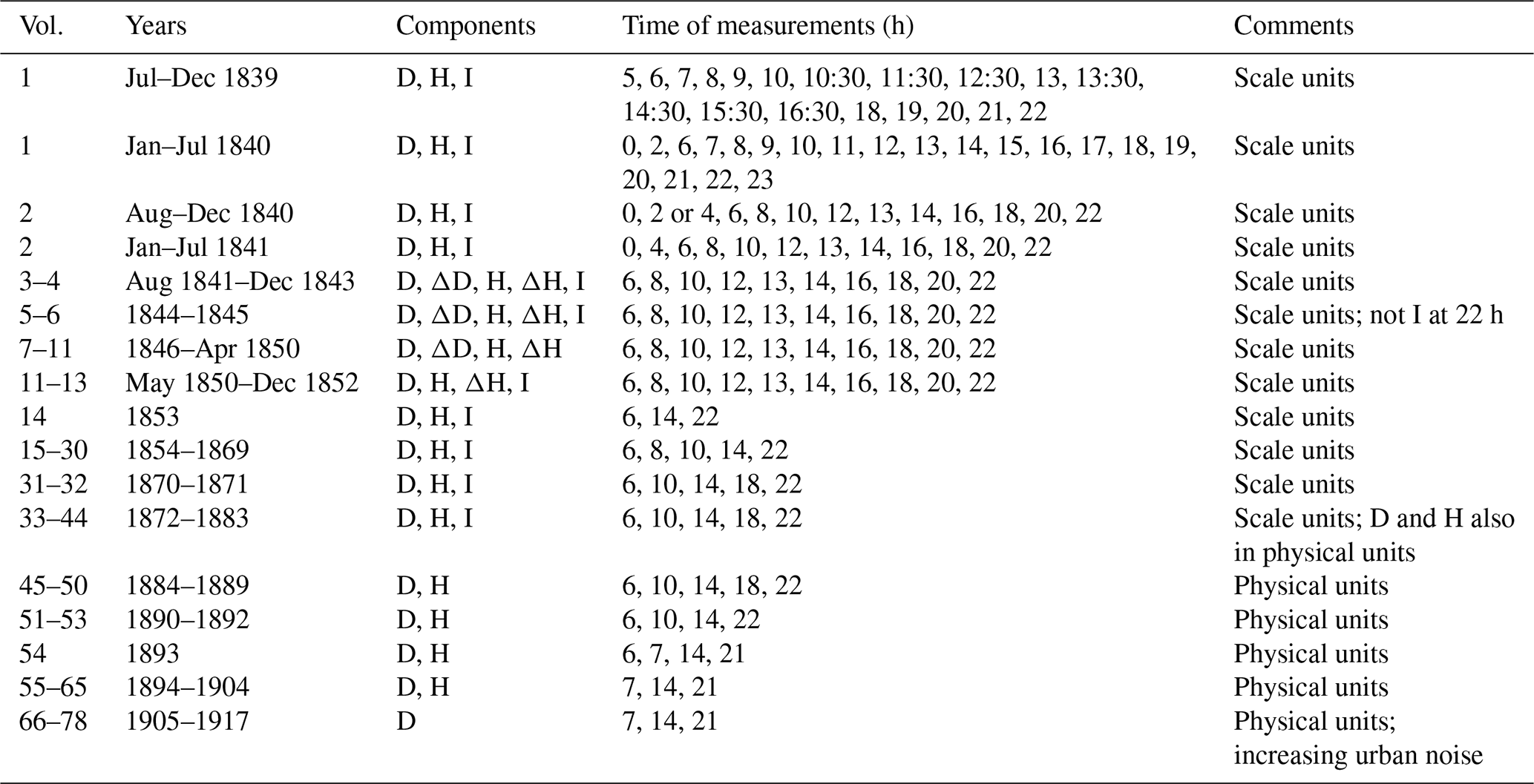
ΔD = difference D(t) – D(t – 5 min), and similarly for ΔH
As the magnetization of the needle is temperature dependent, the temperature inside the case with needle was also recorded; at the beginning this was done twice a day and later during all measurements. Kreil was aware that the temperature dependence of the needle and the issues of the geomagnetic observations in general were not yet sufficiently understood, and that is why the raw data were published in scale units. The data in physical units were published from vol. 33, and publication of scale unit data was stopped in vol. 45. We have decided to digitize first the declination and horizontal intensity data. Transformation of the data available only in scale units to physical units will be reported in the next sections of this paper. The complete data set of the declination from 1839 to 1917 and the horizontal intensity from 1839 to 1904 is provided in the Supplement.
2.3 Records of magnetic disturbances
If the observers on duty noticed an exceptionally fast change in declination or horizontal intensity, they started observations of these components with a higher frequency. The interval between measurements was in the range from 24 s to 10 min, with a typical period of 2 min. About 150 events were recorded from September 1839 to December 1843, which represent 200 full pages in the yearbooks. In the preface to vol. 5, Kreil assessed the existing practice and came to the conclusion that only sufficiently large disturbances are worth being included in the reports in the future. These high-frequency measurements were stopped in 1851 after Kreil left Prague to establish the Central Institution for Meteorological and Magnetic Observations in Vienna. However, the information about disturbed days was not fully omitted. Some brief reports on magnetic storms were published in monthly or yearly summaries. The yearbooks include also observations of the northern lights. They are scattered between the above-mentioned lists of disturbed days and observations of atmospheric phenomena. About 20 observations were recorded in Prague between 1839 and 1905. Thanks to the dark night sky in the 19th century, the polar light was observable even in the city downtown. Information on the polar lights appearances across Europe and North America was also published.
2.4 Term days observations
As mentioned in the introduction, for a short time the Prague observatory joined the simultaneous observations of the magnetic field on selected term days organized by the GMU. A total of 4 term days per year were agreed on from 1839 and started on the Friday preceding the last Saturday of the month, at 22:00 Göttingen civic time, in February, May, August, and November. The observations were carried out at 5 min intervals for 24 h. The results were published in six volumes of the yearbooks Resultate aus den Beobachtungen des Magnetischen Vereins (Gauss and Weber, 1837–1841). The publication of these yearbooks ceased in 1843 after Weber joined the political group called the Göttingen Seven, which protested against constitutional violations of King Ernest Augustus of Hanover, and had to leave Göttingen. Edward Sabine, who coordinated magnetic observatories built up by the government of Great Britain and the East Indian Company, proposed that eight additional simultaneous observations be performed on the Wednesday nearest the 21st day of the eight remaining months, with the hour of commencement being the same as for the GMU (Kreil, 1840b, p. 136–138). Kreil supported the proposal and carried out the term days measurements every month. He continued doing so until the year 1849.
Figure 1, with the time series of magnetic declination, clearly shows the secular variation (a systematic trend in which the orientation of the horizontal projection of the geomagnetic field vector shifts to the east) and a distinct seasonal variation (deviations resembling sinusoids). However, in the period that began sometime in early 1852 and lasted for about 2 years, the course of the declination had a different character than during the rest of the period. This special period begins with a sudden decrease in the size of the declination by about 20 angular minutes; subsequently, the time series continues, as if without a secular variation. Such a course of the magnetic element is unexpected and is most probably also incorrect.
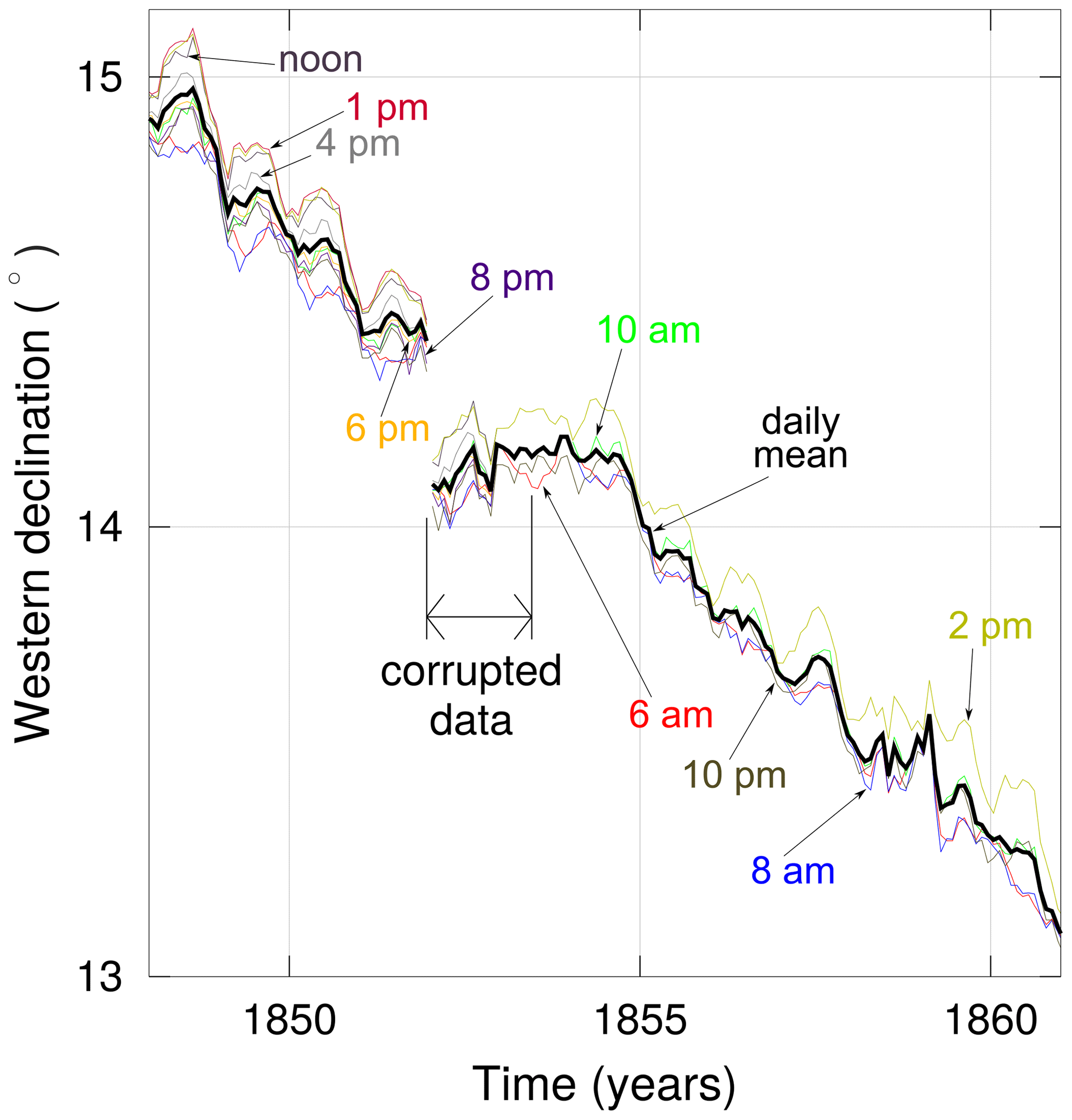
Figure 1Time series of western declination according to observations at the Clementinum observatory in Prague for the period from the beginning of 1848 to the end of 1860. The values measured at different times of the days are plotted in different colours. The times when the measurements were taken is assigned to the individual lines. The average daily values are shown by a thicker black curve. The period with unreliable data in variations of declination (which we discuss in Sect. 3) is pointed out.
Indeed, the yearbook for 1852 (Böhm and Kuneš, 1855, p. IV) also paid attention to this peculiarity. It presents comparisons of the absolute value determined by absolute measurements, with the values determined from the variation apparatus using the formula from the previous year (i.e. from 1851). These comparisons show that the difference between these values have been steadily increasing – almost systematically; in June 1852, the difference ranged from 4 to 5 angular minutes (with a negative sign), and in December it was already more than 12 angular minutes (again with a minus sign). Böhm and Kuneš (1855, p. IV) wrote, “Over the next year, this difference widened without [our] being able to determine its cause, and only later did it become apparent that a spider, which was in the box where the small magnet of the variation apparatus was hung, caused these differences.”
The variations in the yearbook in 1852 and in the first part of 1853 were thus contaminated, likely by a spider web which, in some way, mechanically affected the position of the magnet in the device. There is probably no way to remedy these variations because the spider could have built its web in a way that we have no way of determining. Therefore, we cannot reliably determine the annual averages for the years 1852 and 1853 from those variations. After examining the table comparing the absolute measurements made in June and October 1853 with the absolute data determined from the variations (Böhm and Karlinski, 1856a, p. III), it seems that, for June and October 1853, there are no more systematic deviations between absolute measurements and variations; although there are some differences, they do not seem to be systematic but rather random, with different signs. Therefore, we assume that the variations in the second half of 1853 (including June) are correct.
However, despite the contaminated variation data, we could still obtain some substitute values for the annual averages of absolute declination for 1852 and 1853, which could contain valuable information – more valuable than mere interpolation from existing surrounding annual averages. In the following paragraphs, we explain the way we determined these substitute values.
Although the absolute measurements of 1852 were not found in contemporary sources, there are records available of the differences between the absolute values from variations and from direct measurements (Böhm and Kuneš, 1855, p. IV), such as those which have already been mentioned above. These records were captured on the following days: 22 and 23 June, 6 and 7 July, 21 and 22 October, and 24 December of 1852. Using the formula for converting declination variations to absolute declination and the coefficients which are valid for 1851 together with the records of those calibration measurements, we may easily reconstruct the results of the absolute measurements.
The absolute measurements of declination in June and early July can be interpreted as measured during the summer solstice, the measurements in October are closest to the autumn equinox, and the December measurements are almost exactly at the time of the winter solstice. Figure 2 compares the absolute values at these three time points to the monthly averages in the surrounding periods. We admit that the comparison is not entirely perfect because we have compared the averages of absolute measurements with the monthly averages at 22:00 Göttingen civic time (they should be the least affected by daily variation), but the absolute measurements were made at about 10:00 Göttingen civic time. Even so, we can conclude that the values fit well into the time series. This, to some extent, justifies our belief that the average of the declination calculated from these three instances (14∘17.29′) characterizes the annual average of the declination in 1852. Taking into account the secular variation of per year (assuming a linear trend between the years 1851 and 1854) and the diurnal variation (a relatively subtle difference of 0.11′ between the averages calculated at 22:00 Göttingen civic time and the annual mean; the value found in 1851), a substitute for the annual mean for the centre of the full year of 1852 (i.e. epoch 1852.5) can be estimated, and it gives 14∘18.81′. Note that declination at that time was western in Prague. In accordance with the convention in which the positive direction for the declination is eastern, a negative sign should be added to the value of declination in Prague.
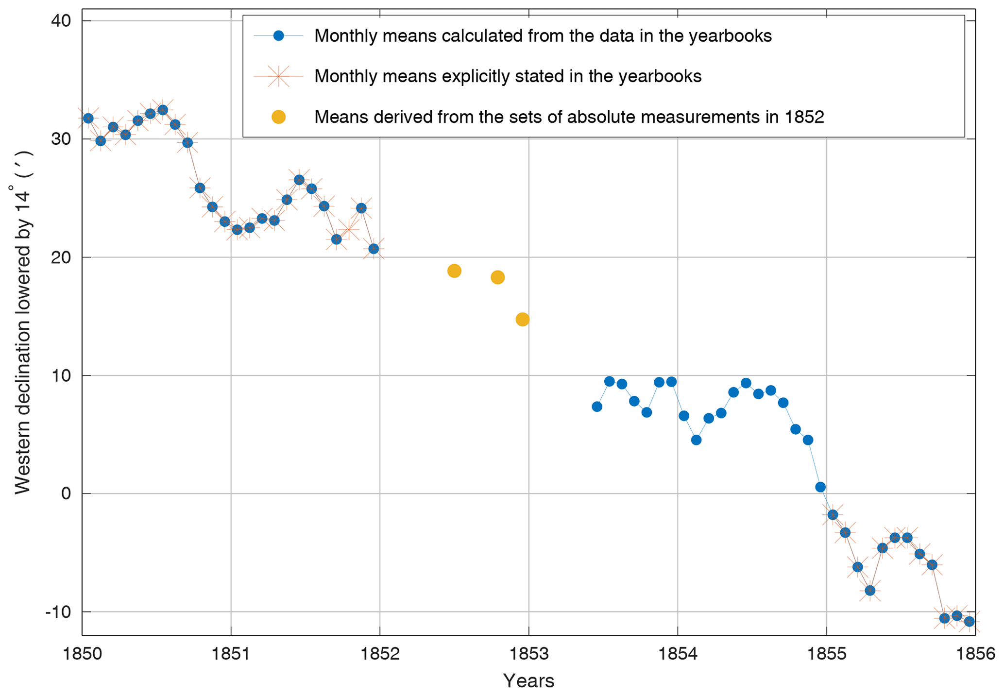
Figure 2Time series of monthly averages of declination (western), which was observed between 1850 and 1855 at the Clementinum observatory in Prague at 22:00 Göttingen civic time. The yellow dots supplement the back-calculated results of the absolute measurements for 1852 at about the time of the summer solstice, the autumn equinox, and the winter solstice.
A substitute value for the annual average of 1853 can be calculated from the monthly averages from June to December 1853 with the addition of the monthly averages of the first 5 months of year 1854. The corresponding data can be found in the yearbooks (Böhm and Karlinski, 1856a, b). From these data, the declination for epoch 1853 (≈1853.92) can be calculated. Then, taking into account the secular variation ( per year), the substitute for the annual mean for the 1853.5 epoch can be obtained. The resulting absolute value of the western declination for this year is thus 14∘12.54′.
The database on the website of the Institute of Geophysics of the Czech Academy of Sciences also preserves the original variation data of the magnetic declination affected by the spider web. Being aware of the limitations of these data, they can still be considered useful for studying rapid variations such as magnetic storms, at least for the purpose of qualitative analysis.
Measurements of horizontal intensity were relatively new at the time of the beginnings of geomagnetic observations in the Prague Clementinum.The methodology of these measurements was invented only a few years before, the absolute method in 1832, and the method for the variations observations in 1837 (e.g. Garland, 1979). It is probable that the novelty of this method caused some ambiguities or imperfections in the first records of these measurements in the Clementinum yearbooks. In this section, we describe some of the problems we encountered while studying the oldest Prague records during the preparation of this article. Solving these problems requires a basic knowledge of the operation of a bifilar magnetometer, which is described below.
4.1 The equation of the bifilar magnetometer
The bifilar magnetometer, the type of an instrument that was used for performing the observations of the horizontal intensity variations in the mid-19th century (Gauss, 1838), has been discussed by Garland (1979) and Nevanlinna (1997).
The main part of the instrument was a large magnetic needle that was suspended by two long fibres (the typical length of the fibres is more than 1 m). The fibres maintained the horizontal position of the needle and, at the same time allowed, the needle to turn in the horizontal plane; as they were very thin and close to each other (a typical distance between them was a few centimetres), they put only a small resistance against the rotary horizontal movement. The length of the needle was about 1 m and its typical weight was of the order of 2 kg. The console from which the fibres hung could revolve around the vertical axis (Fig. 3).
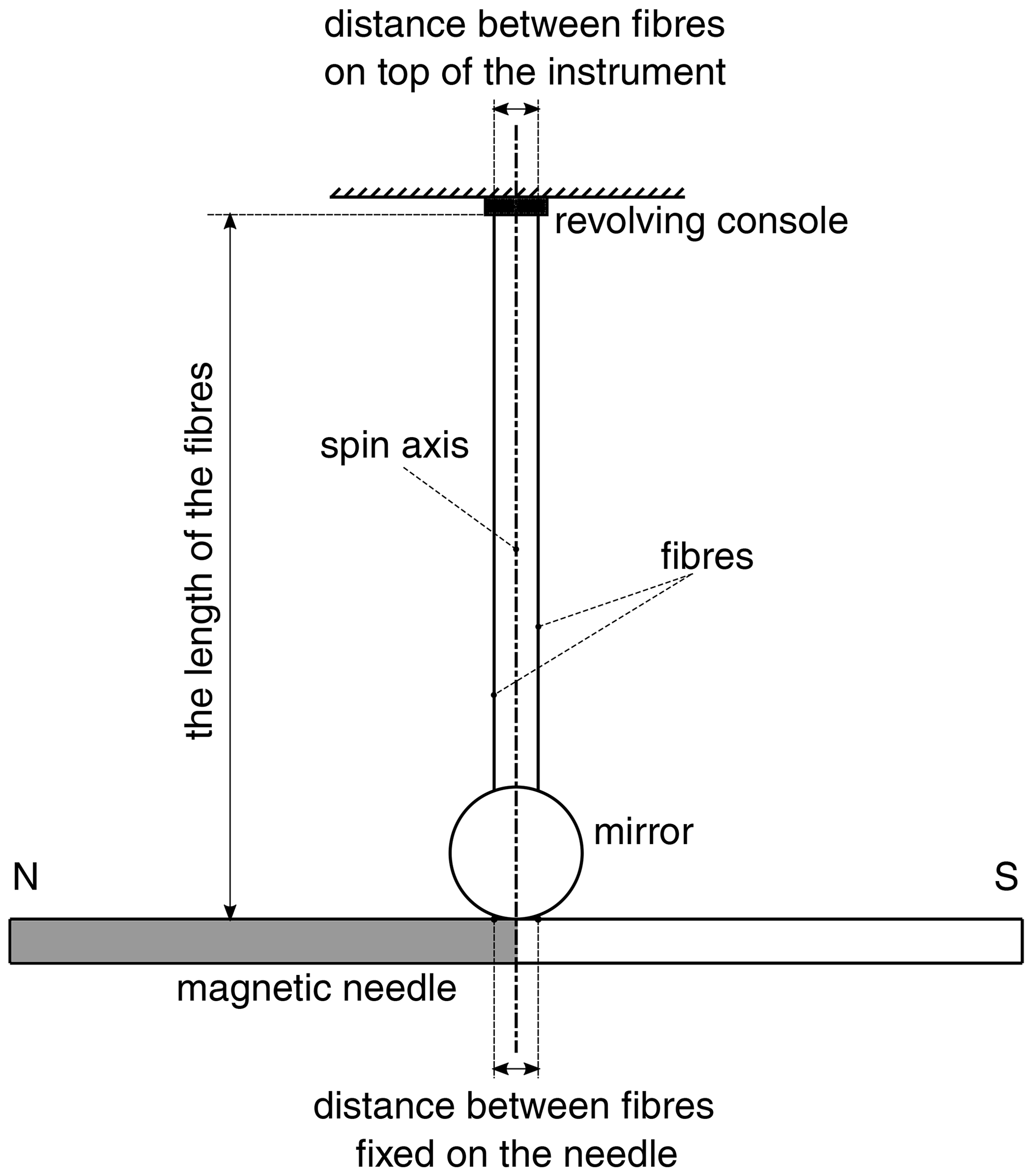
During the initial adjustment of the instrument, the console was revolved so that the magnetic needle came to a position perpendicular to the magnetic meridian. The console was locked in this position.
When there was a small change in the magnitude of the magnetic force which balanced the torque caused by the torsion of the pair of fibres, the magnetic needle slightly deviated from the perpendicular direction in the horizontal plane. In a small mirror, placed on a magnetic needle at the axis of rotation, the reflection of a scale was observed with a telescope with an index line in its objective. It was a scale that was fixed and was placed, for example, on the wall of the room. This made it possible to determine by which angle the needle deviated (Fig. 4).
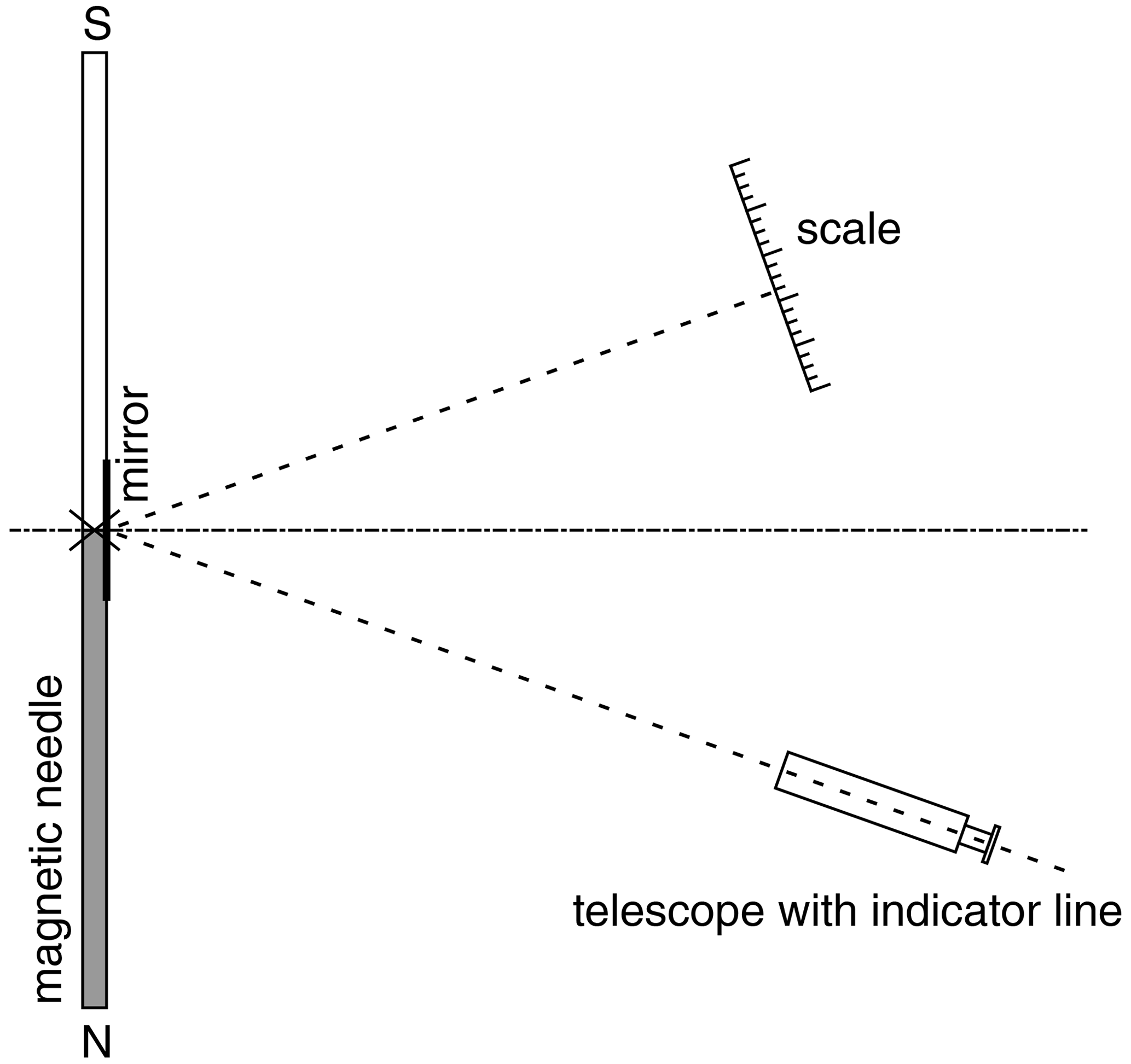
The change in magnetic force could either be due to a change in horizontal intensity or a change in needle magnetization due to a temperature variation. It can be shown (e.g. Nevanlinna, 1997) that the balance between the torsion of a pair of fibres and the rotational effect of a magnetic force yields the following equation:
where H is the absolute value of the horizontal intensity, h0 is the position of the index line observed through the telescope on the scale at the time of the instrument adjustment, and t0 is the temperature of the magnetic needle at the time of the instrument adjustment. At some later time, after the instrument is adjusted, when an observation is being carried out, the position of the index line in the telescope is h, the temperature of the needle is t, and the value of the horizontal intensity differs from the value during the adjustment by ΔH. Equation (1) makes it possible to observe the variations in horizontal intensity by monitoring the position of the index line on the scale and recording the temperature – thus, the bifilar apparatus is a variation device. However, in order to be able to use such a variation device, it is necessary to know the scaling coefficient c1 and the temperature coefficient c2.
In the yearbooks from the Clementinum observatory in Prague, the values of constants c1 and c2 have been explicitly given, together with tables containing the observed index line positions (in scale divisions) and the observed temperatures, but only since 1855. In older yearbooks, only the scaling coefficient was explicitly stated. Although the yearbook (Böhm and Karlinski, 1857, p. XV) contains a record of the calculation of the temperature coefficient for the previous period, in our opinion this calculation is erroneous; moreover, it is valid only after the beginning of 1846, when the older bifilar apparatus was replaced by another apparatus. Therefore, the following two partial problems had to be solved before Eq. (1) could be used:
-
determining the temperature coefficient for the older bifilar apparatus (1 January 1840–31 December 1845);
-
revealing the error or checking the calculation of the temperature coefficient for the newer bifilar apparatus (since 1 January 1846).
In the following section (Sect. 4.2), we will report on the solution of these two tasks.
4.2 Determining the temperature coefficient for the oldest observations of the component H variations
To determine the temperature coefficient c2 for the initial observations of the variations in the horizontal intensity, we can use time series of two quantities which have been recorded in the old yearbooks, i.e. variations in horizontal intensity expressed in divisions of scale h and temperature t expressed in degrees Réaumur (denoted as ∘R; 1 ∘R = 1.25∘C). Temperature t was measured near the magnetometer and represented the temperature of the magnetic needle. The scaling coefficient c1 has been provided in the yearbooks, and we consider its values to be correct.
A similar task, which is to find the temperature coefficient from values of the quantities h and t, was solved for observations at the Helsinki Observatory by Nevanlinna (1997). However, in the case of Helsinki, it was typical that the temperature variations during the day were very large. It was probably due to the fact that their observation room was apparently unheated and insufficiently insulated from the outside environment. This allowed Nevanlinna (1997) to consider the geomagnetic variations during the magnetically quiet days of the winter season to be negligibly small compared to the effect caused by the changes in needle magnetization due to the daily temperature variations. If, during winter quiet days, the changes in h might be considered only as a consequence of temperature variations, the linear regression worked well to estimate the temperature coefficient.
However, in the case of the Clementinum observatory, the situation is different. The thick walls of the building where the observations were performed ensured that the diurnal variation in the temperature of the magnetic needle was almost completely smoothed out. Only a seasonal variation within a 1-year period was observed in the series of temperature inside the observation room.
Because we know that the variations in h caused by the change in needle magnetization were much greater than the variations due to the actual change in magnetic field, we might use a similar approximation than Nevanlinna (1997) on a timescale of several months to years. Also, in our approximation, we considered changes in h only as being a consequence of changes in temperature t, but unlike (Nevanlinna, 1997), they were not the daily variations in the values of h and t but the seasonal variations. This allowed us to use linear regression in the same way to estimate the temperature coefficient.
We also used another simplification, namely we considered only the temperature dependence for the magnetization of the needle. Like Nevanlinna (1997), we did not consider that the magnetization of the rod at any fixed specific temperature could change over time during the studied period. Although the yearbook (Böhm and Karlinski, 1857, p. XV) stated that the magnetism of the rod (needle) “weakened” over time, we think it was an interpretation based on incorrect data. According to our reasoning, the authors of the yearbook confused the physical units in the data on which they based their interpretation. In our opinion, the correct data for the temperature coefficient should be as stated in Table 2. In the yearbook (Böhm and Karlinski, 1857), the authors claimed that they had the absolute magnetic unit per degree of Réaumur. However, based on our analysis in Sect. 4.2, we claim that the figures for all 3 years mentioned (1846, 1849, and 1856) should have been correctly reported in parts of the whole horizontal intensity per degree of Réaumur.1
Table 2The temperature coefficients found in the yearbook (Böhm and Karlinski, 1857, p. XV) and corrected by us afterwards.
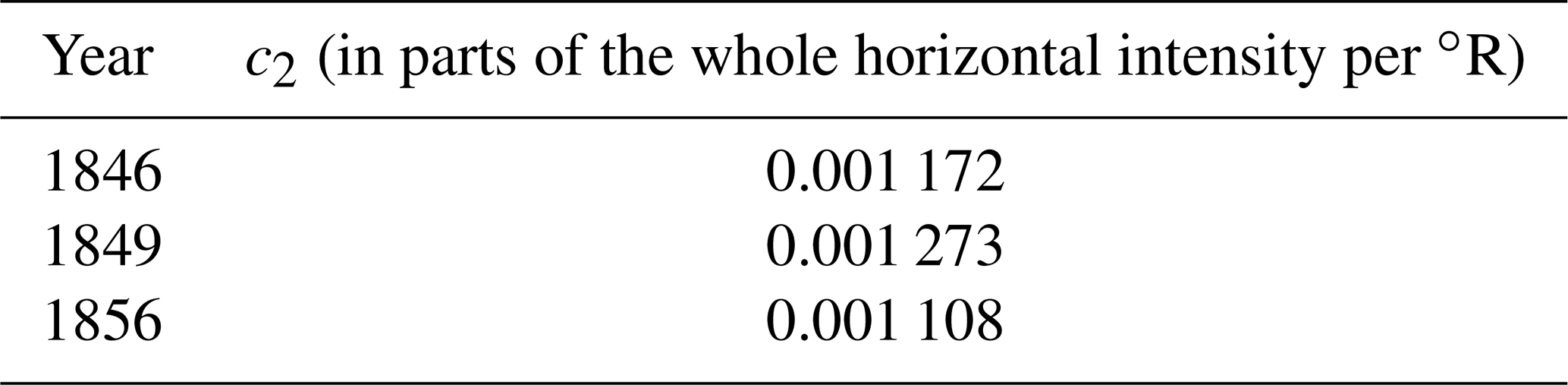
The values in Table 2 do not indicate any systematic increase or systematic decrease in the c2 coefficient; we think that the reason why the listed values differ from each other is rather related to the inaccuracy with which those values were determined. Therefore, we prefer to assume in our study that the c2 coefficient, which stems from the temperature dependence of the needle magnetization, was still approximately the same value for the same needle.
However, from the information in the yearbooks, it can be concluded that two needles or two bifilar devices were used. The first bifilar apparatus was in operation from the beginning of the magnetic measurements at Clementinum until 31 December 1845. On 1 January 1846, another apparatus, which was working with another magnetic needle, was employed. This means that two values of the c2 coefficient have to be determined, with the first of them being valid until the end of 1845 and the second one being valid from the beginning of 1846.
Regarding the first case (i.e. for years 1840–1845), we found no specific mention about the value of coefficient c2 in the yearbooks. Therefore, in Sect. 4.2.1, we calculate it as a new and hitherto unknown numerical value. In the second case, for the period from the beginning of January 1846, three values of the coefficient were given in the yearbooks (we have listed them in Table 2), but we need to dispel doubts about the correctness of these units. The calculations in Sect. 4.2.2 thus serve to verify our assumption of correct units, rather than to determine some other numerical value.
4.2.1 Calculating the temperature coefficient for the bifilar apparatus until 31 December 1845
We estimated the value of the temperature coefficient for the period from 1 January 1840 to 31 December 1845 for six isolated time periods between which, according to notes in the yearbooks, the setting of the bifilar apparatus was changed. The readjustment of the apparatus was probably performed for the following two reasons:
-
the fibres on which the needle was suspended had ruptured,
-
the instrument had to be repositioned due to the secular variation and, as a result, the deviation in the magnetic needle systematically increased to the limit of the measuring range of the instrument.
Using coefficient c1, the values of which we read from the yearbooks, we converted the variations given in the scale divisions to the numerical values given in the parts of the whole horizontal intensity.
Subsequently, we calculated temperature coefficients for individual periods using the method of least squares. In doing so, we determined the parameters of the function as follows:
In this linear equation, c2 is the temperature coefficient sought, and c3 is the parameter which determines the value of the fraction at the temperature (the specific value of c3 is of no interest for this study). The obtained values of the temperature coefficient for the period 1840–1845 are given in Table 3. According to these data, the mean of the temperature coefficient is as follows:
Since we do not have another estimate of the temperature coefficient for the very first years of observations in Clementinum, we will use this numerical value in further calculations (Sect. 4.3).
Table 3The values of the temperature coefficient c2 for six continuous periods from the beginning of 1840 to the end of 1845.

4.2.2 Verification of the temperature coefficient of the bifilar apparatus from 1846 to 1854–1855
Even from 1 January 1846, when a new bifilar apparatus was used for observations of horizontal intensity, until the end of 1854, the values of the temperature coefficient were not given in the yearbooks. In the 1855 yearbook, the temperature coefficients were back-calculated, but due to uncertainties about the physical units in which their results were given, we considered it necessary to verify them with our own calculations. We proceeded in the same way as in Sect. 4.2.1.
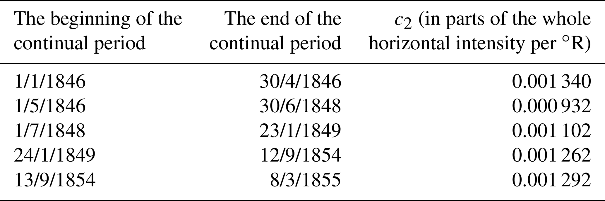
For the period from the beginning of 1846 to 8 March 1855, we had five continuous time periods at our disposal for which we determined the temperature coefficient, satisfying Eq. (2) by the method of least squares. The partial values are listed in Table 4.
Table 4The values of the temperature coefficient c2 for continuous periods during 1840–1845.
The mean value for the temperature coefficient calculated from the data in Table 4 is as follows:
The value that we obtained is in good agreement with the corrected data stored in Table 2. After this verification, the numerical values in Table 2, or rather their mean value, may be taken as the temperature coefficient for the whole period from 1 January 1846 to 31 December 1854 as follows:
We will use this value in Sect. 4.3 in our calculations for the period up to the time when the values of the temperature coefficient are provided in the yearbooks (in the headers of tables that contain the variations given in scale divisions).
4.3 A baseline for the horizontal intensity in years 1840–1854 and the annual means
At the beginning of the geomagnetic observations at Clementinum, the following two types of measurements were performed:
-
occasional measurements of the whole horizontal intensity by means of the Gauss absolute method;
-
regular observations of the variations in the horizontal intensity (expressed in parts of the whole horizontal intensity).
These two types of measurements were linked only by the fact that observers needed a value of the total horizontal intensity to express variations in horizontal intensity in absolute units. However, in contrast to practices nowadays, the baselines of the variation apparatus were not calculated afterwards. Therefore, in this section, we will calculate the baseline for the period from 1840 to 1854. From 1855, the yearbooks provide the baseline values (under the designation of “constant”).
To calculate the values of the baseline, we followed the procedure that became the standard method used today, i.e. we compared the trends in the time series of registered variations in horizontal intensity (only the pure variations with no baseline added) with the values of horizontal intensity determined by absolute measurements. The time series of the registered variations with no baseline added were calculated for each of the continual periods separately (Tables 3 and 4). Using the tabulated variations, which are provided by the yearbooks in scale divisions, together with scaling coefficient c1 and temperature coefficient c2, we obtained the values for the variations of the horizontal intensity expressed in the absolute units.
Figure 5a shows that there are some instances in the time series when the values change abruptly. These are the discontinuities due to readjustments of the bifilar device. In one case, namely between 30 December 1845 and 1 January 1846, the abrupt change was caused by the replacement of the old bifilar instrument with a new one. In the next step, we therefore treated the discontinuities in the time series. We did it by manually moving the entire continuous section of the time series in a vertical direction so that we connected the ends of the previous sections with the beginnings of the following sections. The resulting continuous time series is shown in Fig. 5b, where the values are given in the absolute units of Gauss's original unit system that was based on mm–mg–s (millimetre, milligram, and second). By multiplying those numerical values by a factor of 10 000, the original unit can be changed to a modern nanotesla unit.
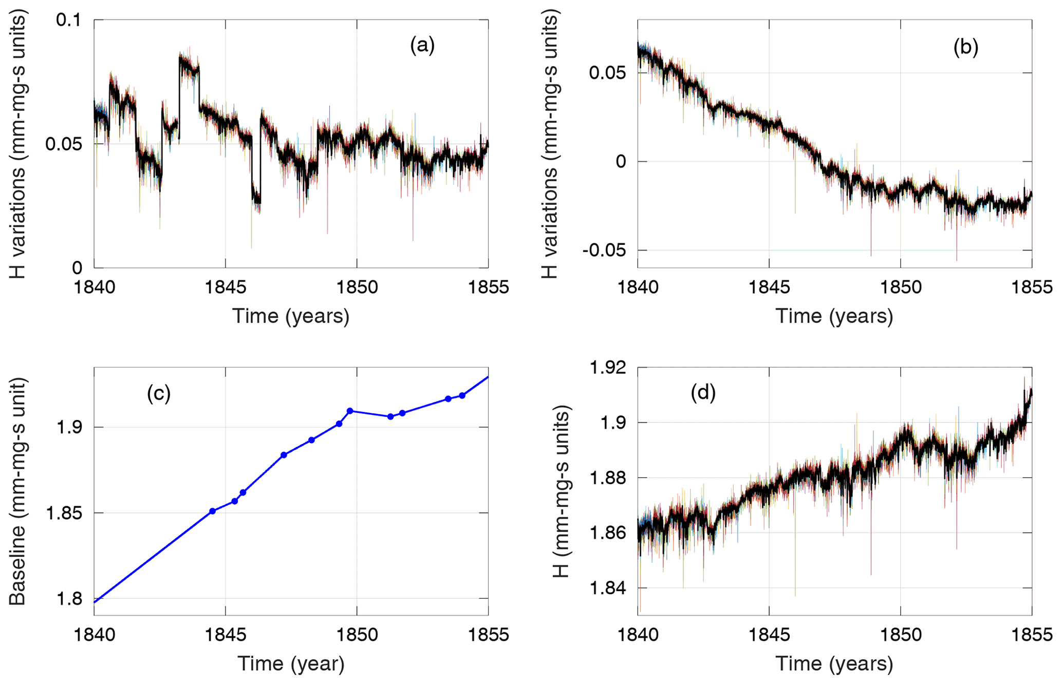
Figure 5The horizontal intensity in Prague (Clementinum) from the beginning of 1840 until the end of 1854. (a) The variations, as recorded in the yearbooks, converted to the physical unit of the mm–mg–s (millimetre, milligram, and second) system introduced by Gauss. Discontinuities that arose at the time when the settings of the bifilar apparatus were performed are not yet removed from the time series. The discontinuity between 1845 and 1846 arose from the replacement of the old apparatus with a new one. The values measured at different parts of the days are plotted in different colours. The average daily values are shown by a thicker black curve. (b) The time series after the removal of the discontinuities. (c) The baseline of the instrument that was used for measuring the variations in the horizontal intensity. (d) Time series of absolute values of the horizontal intensity at the Clementinum observatory for the period 1840–1854.
Other necessary data are the results of absolute measurements of the horizontal intensity. Figure 6 displays the data of the absolute measurements that we found in the yearbooks. A comparison with the course of the data of the Munich Observatory, which is only 300 km away from Prague, shows, at first sight, that the absolute measurements before 1844 deviate from what we would expect. A confrontation with the gufm1 model (Jackson et al., 2000) also shows that the absolute measurements in the first years of geomagnetic observations in Prague were probably characterized by a disproportionately large error, most likely systematic observational error. Therefore, for this period, we preferred to use the value of horizontal intensity, which we obtained by extrapolation based on a linear regression of the data between 1844 and 1853.
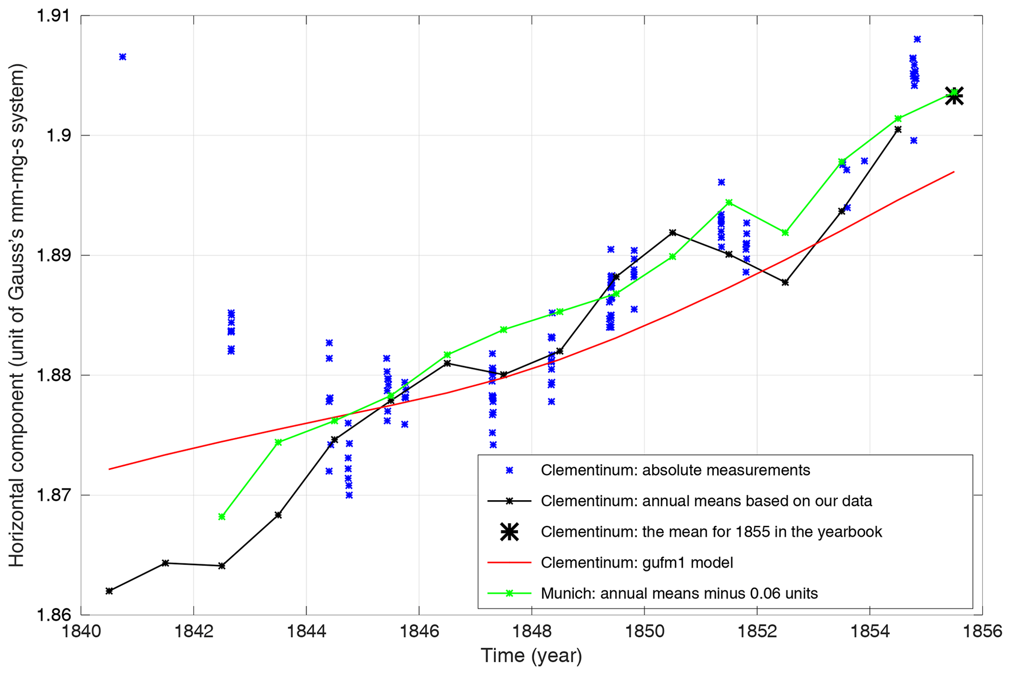
Figure 6The comparison of the absolute values of the horizontal intensity observed at Clementinum (absolute measurements – blue; annual means calculated by us – black curve; the annual mean for 1855 taken from the yearbook – black asterisk) with the annual means of the horizontal intensity in Munich reduced by 600 nT (i.e., 0.06 absolute units in mm–mg–s). The red curve is the horizontal intensity for Prague provided by the gufm1 model (Jackson et al., 2000).
The final baseline that we then obtained is presented in Fig. 5c. We also need to mention that, to determine the baseline, we used the variation data that were observed at 16:00 Göttingen civic time because absolute measurements in the first years of the observatory's operation were usually performed around 16:00 Göttingen civic time, which is based on the information found in the yearbooks.
By adding the baseline values to the time series of the variations, we obtained a time series of the absolute values of the horizontal intensity (Fig. 5d). From these data, we then calculated the annual means of the horizontal intensity for Prague (see data in Table 5). A comparison of the annual means that we obtained (Fig. 6) with the annual averages from Munich (data taken from the World Data Centre of Geomagnetism, Edinburgh) indicates a good agreement in the trend of the time series at these two not-too-far-away observatories. We believe that this good agreement can be considered a confirmation of the correctness of the calculations we made in Sects. 4.2 and 4.3.
Table 5Annual means of the horizontal intensity at the Clementinum observatory in Prague in the first years of its operation.

In addition to obtaining the time series that capture the secular variations in the geomagnetic field, the study of historical records from old observatories has another, at least equally important, benefit. This benefit is related to records of intense magnetic storms that occurred in the 19th century. As an example of such a record, we show here the course of the horizontal intensity during an interesting magnetic storm which commenced on the evening of 3 September 1839. Subsequently, after midnight and in the early morning time, two sudden, relatively deep, and short-lasting drops in horizontal intensity appeared in the Prague records (Fig. 7a). It is probable that these two swift variations were local phenomena, possibly substorms or some other variations that were caused by electric currents in the auroral oval. Here we assume that the auroral oval reached as far as central Europe at that time. Our assumption that the auroral oval was located in relatively low geographical (or magnetic) latitudes around 3 September 1839 is based on observations recorded in a little-known document (Snow, 1842) from the first half of the 19th century.
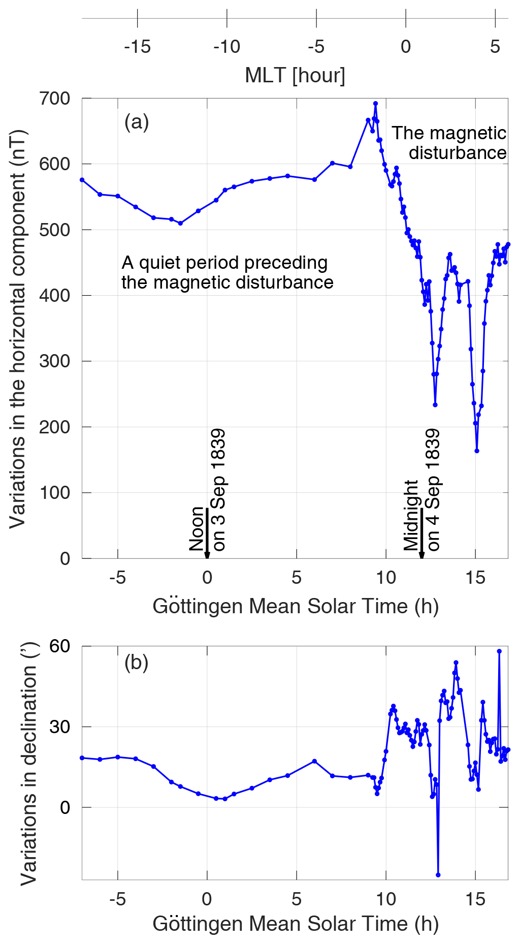
Figure 7The first storm that was registered at Clementinum. It commenced on 3 September 1839 in the evening. (a) There were two sharp and deep depressions of the horizontal intensity that occurred after midnight on 4 September 1839 at 12:45 and 15:05 (Göttingen mean solar time). These moments correspond to magnetic local times 01:39 and 04:59, respectively. Judging from their shapes and from the fact that they happened at night, these two swift disturbances might probably have been substorms. The figure also demonstrates the procedure with which the magnetic storms were commonly registered that time, i.e. shortening the time interval between readings of the values from the variation instruments immediately after an interesting magnetic variation commenced, as described in Sect. 2.3. Panel (b) displays the course of (eastern) declination during the same period.
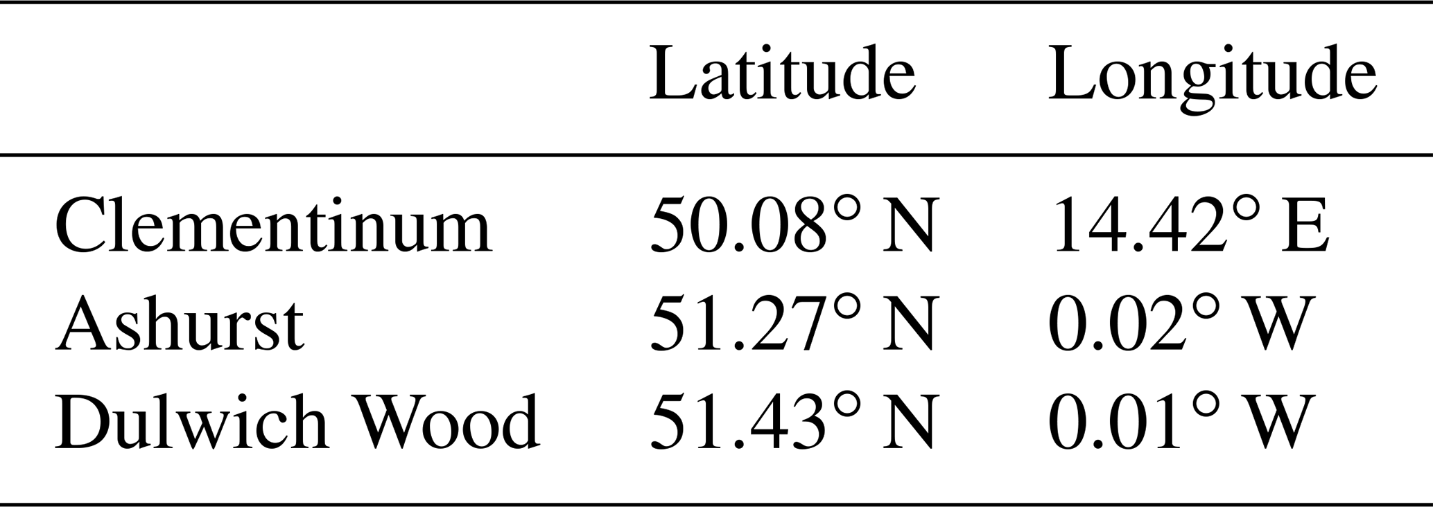
Robert Snow, who observed the northern lights from September 1834 to September 1839, reported the event which occurred on 3 September 1839. He claimed that this was the second most beautiful aurora borealis he had ever observed (Snow, 1842, p. 15). He made observation of this event at Ashurst in West Sussex, England (51∘16′ N, 0∘1′10′′ W). The geographical latitudes of Prague and Ashurst differ by 14.4∘ (Table 6). The difference between the local times of these two places is, thus, about 1 h. Although this particular geomagnetic disturbance and the accompanying aurora borealis are not well known to the scientific community today, Snow (1842) states that the press at the time were informed about this aurora.
Table 6Geographical coordinates of Clementinum, Ashurst, and Dulwich Wood – another place which Robert Snow used for his observations of the auroras that he reported in (Snow, 1842); this place is situated in southern London.
The aurora borealis accompanying the magnetic storm of 3 and 4 September 1839 was also observed in Prague. However, Kreil (1840b) writes that they could not pay full attention to observing this phenomenon because they measured the magnetic field, namely declination and horizontal intensity, all the time.
The measuring range of the bifilar device in Prague was large enough to detect the storm on 3 December 1839. Also, the conversion of the scale divisions to parts of the horizontal intensity (see Eq. 1) was sufficiently accurate for this case. This even applies during the deepest depression in the horizontal intensity of about 400 nT (the second of the violent variations at 15:05 Göttingen mean time, which represents 03:05 Göttingen civic time; see Fig. 7a). The good accuracy was ensured despite that, in deriving the Eq. (1), an approximate relation tan φ∼φ was used for the tangent of the angle by which the magnetic rod deflected during the depression of the horizontal intensity; this approximation allowed the equation to be written in a simple linear form. In more precise calculations, the above-mentioned 400 nT should only be corrected by less than 1 nT. The device would hypothetically manage to record such a large decrease in horizontal intensity, as was observed in Colaba on 2 September 1859 (ΔH∼1600 nT according to Tsurutani et al., 2003). In fact, at that time in Colaba, a measuring apparatus operating on the same principles was used. However, with such a large depression, the results obtained from Eq. (1) for the Prague apparatus would need a correction exceeding 10 nT. With even larger deviations in ΔH, the required correction would continue to increase nonlinearly. We note that the horizontal intensity during the event on 2 September 1859 was not recorded in Prague because the deflection of the magnetic rod at the time of the depression of the geomagnetic field simply came out of the insufficient scale range of the instrument.
During the remarkable event on 3 September 1839 in Prague, magnetic declination was also recorded incessantly (Fig. 7b). The record shows that the short-lasting drops in horizontal intensity were accompanied by short and swift negative perturbations in declination. If we assume that these perturbations were related to the downward-oriented, field-aligned currents that were parts of substorm current wedges, Prague would have been located near the outside edge of the auroral oval that time. There are gaps in the inclination records during this event; data are not available at all during the first of the possible substorms. During the second possible substorm (i.e. during the second swift, short drop in horizontal intensity), a short-term increase in inclination of about a quarter of a degree can be inferred.
Other examples of interesting geomagnetic disturbances observed in the Clementinum are the extreme variations in the magnetic field that occurred on 17 November 1848 and 4 February 1872 (Valach et al., 2019). We believe that the digitized records from the Clementinum observatory of Prague will provide an opportunity to study other interesting events.
The presented study can be primarily conceived as a presentation of the unique database collected from geomagnetic recording at the Clementinum observatory in Prague during the 19th century. From another point of view, this study can serve as an example of how to deal with historical geomagnetic data in context with current research trends in geomagnetism. It is also documented here that putting the records in proper physical units and coping with data inconsistencies is an essential part of the research.
In dealing with proper scaling of the historical geomagnetic records, this study partly builds on earlier work by Nevanlinna (1997). The major outcome of these efforts is the proper adjustment of thermal coefficient in the equation for bifilar magnetometer. Having this constant determined, it is possible to rescale the data in geomagnetic records and to reconstruct the time series for horizontal intensity. As such, the adopted geomagnetic records can be cast in consistent forms to serve as a reliable source of information for research purposes. As detailed in the main part of this paper, the procedure of computing the temperature dependence here, in some sense, can be considered as complementary to that in Nevanlinna (1997).
Closer study of the early Clementinum data reveals an interesting magnetic disturbance which is nearly unknown and almost forgotten in the present-day geomagnetic community. There is an indication that this disturbance can be interpreted as being caused by currents related to the auroral oval transiently extending to midlatitudes. We proposed that this disturbance could be identified as two subsequent magnetic substorms.
Our database has the potential to add valuable information to existing global geomagnetic data resources. Recently, for instance, the HISTMAG database was created by Arneitz et al. (2017b), consisting of large amounts of palaeomagnetic and archaeomagnetic data and a rich collection of instrumental historical observations. Compiling the historical data from several observatories can be helpful in dealing with inconsistencies or missing data. The study of multiple records is also necessary for a more global view of a considered geophysical phenomenon, in contrast to the study of data from a single location on the Earth's surface. For example, in Valach et al. (2019), the Clementinum data together with the geomagnetic records from other observatories have been used to analyse selected strong geomagnetic disturbances.
In a broader context, the scientific benefit of the presented work can be twofold. First, using the properly scaled series of geomagnetic records, the long-term behaviour of the geomagnetic field at the Clementinum observatory can be reconstructed. These data, along with historical data from other observatories combined with some supplementary (archaeomagnetic, palaeomagnetic) data, can be useful for modelling the global secular variation. Second, the consistent historical magnetic record supported with some other sources of data (e.g. records of aurorae) can be searched for extreme geomagnetic disturbances (magnetic storms and substorms). This kind of approach can make a contribution to the study of extreme space weather events.
The final digital data of the magnetic declination and horizontal intensity given in physical units are available in the Supplement.
The supplement related to this article is available online at: https://doi.org/10.5194/angeo-39-439-2021-supplement.
PH devised the idea of the study, organized the scan of yearbooks and data digitization, carried out primary data processing and transformation of declination to physical units, and checked the consistency of the final data. FV calculated and verified the temperature coefficients for the bifilar magnetometer during the years 1840–1854, participated in the transformation of the horizontal intensity to physical units, and pointed out the event on 3 September 1839. MR helped with the introductory and concluding sections, amended the whole text, and checked the paper.
The authors declare that they have no conflict of interests.
Pavel Hejda thanks to Leif Swalgaard (Stanford University) who drew his attention to the old magnetic observatory data. Thanks also go to the National Centers for Environmental Information (NCEI) for operating the online magnetic field calculators (https://www.ngdc.noaa.gov/geomag/calculators/magcalc.shtml#igrfwmm, last access: 10 May 2021), which we used in our study, and to the World Data Centre of Geomagnetism (Edinburgh) for collecting and maintaining annual averages from historical observatory in Munich (http://www.geomag.bgs.ac.uk/data_service/data/annual_means.shtml, last access: 10 May 2021).
This research has been supported by the Vedecká Grantová Agentúra MŠVVaŠ SR a SAV (grant no. 2/0085/21).
This paper was edited by Nick Sergis and reviewed by two anonymous referees.
Alexandrescu, M., Courtillot, V., and Le Mouël, J. L.: Geomagnetic field direction in Paris since the mid-sixteenth century, Phys. Earth Planet. In., 98, 321–360, 1996. a
Arneitz, P., Egli, R., and Leonhardt, R.: Unbiased analysis of geomagnetic data sets and comparison of historical data with paleomagnetic and archeomagnetic records, Rev. Geophys., 55, 5–39, 2017a. a
Arneitz, P., Leonhardt, R., Schnepp, E., Heilig, B., Mayrhofer, F., Kovacs, P., Hejda, P., Valach, F., Vadasz, G., Hammerl, C., Egli, R., Fabian, K., and Kompein, N.: The HISTMAG database: combining historical, archaeomagnetic and volcanic data, Geophys. J. Int., 210, 1347–1359, 2017b. a, b
Böhm, J. G. and Karlinski, F.: Magnetische und meteorologische Beobachtungen zu Prag, Zechzehnter Jahrgang: Vom 1. Jänner bis 31. December 1853, Druck der k. k. Hofbuchdruckerei von Gottlieb Haase Söhne, Prag, Czech Republic, 1856a. a, b
Böhm, J. G. and Karlinski, F.: Magnetische und meteorologische Beobachtungen zu Prag, Zechzehnter Jahrgang: Vom 1. Jänner bis 31. December 1854, Druck der k. k. Hofbuchdruckerei von Gottlieb Haase Söhne, Prag, Czech Republic, 1856b. a
Böhm, J. G. and Karlinski, F.: Magnetische und meteorologische Beobachtungen zu Prag, Zechzehnter Jahrgang: Vom 1. Jänner bis 31. December 1855, Druck der k. k. Hofbuchdruckerei von Gottlieb Haase Söhne, Prag, Czech Republic, 1857. a, b, c, d
Böhm, J. G. and Kuneš, A.: Magnetische und meteorologische Beobachtungen zu Prag, Dreizehnter Jahrgang: Vom 1. Jänner bis 31. December 1852, Druck der k. k. Hofbuchdruckerei von Gottlieb Haase Söhne, Prag, Czech Republic, 1855. a, b, c
Cafarella, L., De Santis, A., and Meloni, A.: Secular variation in Italy from historical geomagnetic field measurements, Phys. Earth Planet. In., 73, 206–221, 1992. a
Cnossen, I. and Matzka, J.: Changes in solar quiet magnetic variations since the Maunder Minimum: A comparison of historical observations and model simulations, J. Geophys. Res.-Space, 121, 10520–10535, https://doi.org/10.1002/2016JA023211, 2016. a
Dobrica, V., Demetrescu, C., and Mandea, M.: Geomagnetic field declination: from decadal to centennial scales, Solid Earth, 9, 491–503, https://doi.org/10.5194/se-9-491-2018, 2018. a
Garland, G. D.: The contributions of Carl Friedrich Gauss to geomagnetism, Hist. Math., 6, 5–29, 1979. a, b
Gauss, C. F.: Intensitas vis magneticae terrestris ad mensuram absolutam revocata, 205, 2041–2058, Göttingische Gelehrte Anzeigen, Göttingen, Germany, 1833. a, b
Gauss, C. F.: Bemerkungen über die Einrichtung und den Gebrauch des Bifilar-Magnetometers, in: Resultate aus den Beobachtungen des Magnetischen Vereins im Jahre 1837, edited by: Gauss, C. F. and Weber, W., Verlage der Dieterichschen Buchhandlung, Göttingen, Germany, 20–37, 1838. a
Gauss, C. F. and Weber, W. E.: Resultate aus den Beobachtungen des Magnetischen Vereins, Verlage der Dieterichschen Buchhandlung, Göttingen, Germany, 1837, 1838; Verlage der Weidmannschen Buchhandlung, Leipzig, Germany, 1839, 1840, 1841, 1843. a
Gubbins, D. and Herrero-Bervera, E. (Eds.): Encyclopedia of Geomagnetism and Paleomagnetism, Springer, Dordrecht, The Netherlands, 2007. a
Jackson, A., Jonkers, A. R., and Walker, M. R.: Four centuries of geomagnetic secular variation from historical records, Philos. T. Roy. Soc. A, 358, 957–990, 2000. a, b, c
Jonkers, A. R., Jackson, A., and Murray, A.: Four centuries of geomagnetic data from historical records, Rev. Geophys., 41, 1006, https://doi.org/10.1029/2002RG000115, 2003. a
Korte, M., Mandea, M., and Matzka, J.: A historical declination curve for Munich from different data sources, Phys. Earth Planet. In., 177, 161–172, 2009. a, b
Kreil, K.: Magnetische und meteorologische Beobachtungen zu Prag, in: Zeitschrift für Physik und verwandte Wissenschaften, Sechter Band, Dr. Philipp Ritter von Holger, Wien, Austria, 117–138, 1840a. a
Kreil, K.: Magnetische und meteorologische Beobachtungen zu Prag, in: Zeitschrift für Physik und verwandte Wissenschaften, Sechter Band, Dr. Philipp Ritter von Holger, Wien, Austria, 18–37, 1840b. a
Lockwood, M., Owens, M. J., Barnard, L. A., Scott, C. J., and Watt, C. E.: Space climate and space weather over the past 400 years: 1. The power input to the magnetosphere, J. Space Weather Spac., 7, A25, https://doi.org/10.1051/swsc/2017019, 2017. a
Lockwood, M., Owens, M. J., Barnard, L. A., Scott, C. J., Watt, C. E., and Bentley, S.: Space climate and space weather over the past 400 years: 2. Proxy indicators of geomagnetic storm and substorm occurrence, J. Space Weather Spac., 8, A12, https://doi.org/10.1051/swsc/2017048, 2018. a
Malin, S. C. R. and Bullard, E.: The direction of the Earth's magnetic field at London, 1570–1975, Philos. Tr. R. Soc. S.-A, 299, 357–423, 1981. a
Matzka, J., Chulliat, A., Mandea, M., Finlay, C. C., and Qamili, E.: Geomagnetic observations for main field studies: from ground to space, Space Sci. Rev., 155, 29–64, 2010. a
Nevanlinna, H.: Gauss' H-variometer at the Helsinki Magnetic Observatory 1844–1912, J. Geomagn. Geoelectr., 49, 1209–1215, 1997. a, b, c, d, e, f, g, h, i
Pro, C., Vaquero, J. M., and Merino‐Pizarro, D.: Early geomagnetic data from the Astronomical Observatory of Madrid (1879–1901), Geosci. Data J., 5, 87–93, 2018. a
Ptitsyna, N. G., Sokolov, S. N., Soldatov, V. A., and Tyasto, M. I.: Historical Database of Geomagnetic and Auroral Activity for the Study of Solar-Terrestrial Relationships, Izv. Atmos. Ocean. Phy.+, 54, 730–737, 2018. a
Reay, S. J., Herzog, D. C., Alex, S., Kharin, E. P., McLean, S., Nosé, M., and Sergeyeva, N. A.: Magnetic observatory data and metadata: Types and availability, in: Geomagnetic observations and models, Springer, Dordrecht, The Netherlands, 149–181, 2011. a
Schröder, W. and Wiederkehr, K. H.: A history of the early recording of geomagnetic variations, J. Atmos. Sol.-Terr. Phy., 62, 323–334, 2000. a
Snow, R.: Observations of the Aurora Borealis from September 1834 to September 1839, Noyes and Barclay, Castle Street, Leicester Square, London, UK, 1842. a, b, c
Svalgaard, L.: Observatory Data: a 170-year Sun-Earth Connection, in: Proceedings of the XIIIth IAGA Workshop on geomagnetic observatory instruments, data acquisition, and processing, 9–18 June 2008, Boulder, Colorado, USA, edited by: Love, J. J., US Geological Survey Open-File Report 2009–1226, 246–257, 2009. a
Svalgaard, L.: How well do we know the sunspot numbers?, in: Presentation at Colloquium at High Altitude Observatory, Boulder, Colorado, USA, available at: https://www.leif.org/research/ (last access: 10 May 2021), 2012. a
Tsurutani, B. T., Gonzalez, W. D., Lakhina, G. S., and Alex, S.: The extreme magnetic storm of 1–2 September 1859, J. Geophys. Res., 108, 1268, https://doi.org/10.1029/2002JA009504, 2003. a
Valach, F., Hejda, P., Revallo, M., and Bochníček, J.: Possible role of auroral oval-related currents in two intense magnetic storms recorded by old mid-latitude observatories Clementinum and Greenwich, J. Space Weather Spac., 9, A11, https://doi.org/10.1051/swsc/2019008, 2019. a, b, c
Wolf, R.: Mittheilungen über die Sonneflecken IX, in: Vierteljahrsschrift der Naturvorschenden Gesellschaft in Zürich, Zurich, Switzerland, 213–252, 1859. a
Wolf, R.: Mittheilungen über die Sonneflecken XI, in: Vierteljahrsschrift der Naturvorschenden Gesellschaft in Zürich, Zurich, Switzerland, 233–271, 1860. a
Wolfer, A.: Astronomische Mittheilungen, CIV. Astron. Mitteil. Eidgn. Sternw. Zürich, 11, 89–114, 1914. a
In some places, there are errors in the yearbook when the value in parts of the whole horizontal intensity is given instead of the value in absolute units. The error can be eliminated by multiplying by 1.9, which is the value of the then horizontal intensity in absolute units of the system mm–mg–s (millimetre, milligram, and second) introduced by Carl Friedrich Gauss.
- Abstract
- Introduction
- Database of the Clementinum magnetic data
- Corrupted data of magnetic declination around the year 1852
- Horizontal intensity in the first years of the Clementinum observations
- An example of recorded strong magnetic disturbances – the event on 3 September 1839
- Conclusions
- Data availability
- Author contributions
- Competing interests
- Acknowledgements
- Financial support
- Review statement
- References
- Supplement