


Abstract
Significant innovations in next-generation sequencing techniques and bioinformatics tools have impacted our appreciation and understanding of RNA. Practical RNA sequencing (RNA-Seq) applications have evolved in conjunction with sequence technology and bioinformatic tools advances. In most projects, bulk RNA-Seq data is used to measure gene expression patterns, isoform expression, alternative splicing and single-nucleotide polymorphisms. However, RNA-Seq holds far more hidden biological information including details of copy number alteration, microbial contamination, transposable elements, cell type (deconvolution) and the presence of neoantigens. Recent novel and advanced bioinformatic algorithms developed the capacity to retrieve this information from bulk RNA-Seq data, thus broadening its scope. The focus of this review is to comprehend the emerging bulk RNA-Seq-based analyses, emphasizing less familiar and underused applications. In doing so, we highlight the power of bulk RNA-Seq in providing biological insights.
Introduction
Transcriptomics provides deep insights into both coding and non-coding regions functional properties, helping understand various cellular conditions or disease phenotypes. Using these analyses, one can study differential gene expression across tissues or patient cohorts, perform isoform analysis and investigate splicing events across genes. To date, RNA sequencing (RNA-Seq) has been used in many fields including healthcare [1, 2], agriculture [3, 4], microbial diversity [5] and evolutionary biology [6], proving its usefulness in various applications [7]. As these fields have expanded, different biological challenges have pushed the development of novel computational tools that have evolved and diversified according to technological advancements, leading to many novel applications using bulk RNA-Seq. Bulk RNA-Seq measures the transcriptomics of pooled cell populations, tissue sections or biopsies.
Given the bespoke nature of many of the newer bulk RNA-Seq applications, widespread use can be impacted by lack of familiarity or propagation between research groups. For example, for copy number alteration (CNA) and indel detection, DNA analysis (as targeted, exome or genome sequencing) is extensively used in cancer research. Newly developed bioinformatic tools and integrated interpretational methods for RNA-Seq have the potential to perform and explain those analyses with better accuracy than before, in scenarios where whole genome sequencing (WGS) is not available because of limited resources. Other RNA-Seq applications with expanding utility include detection of microbial contamination in experiments [8], the understanding of transposable elements (TEs) [9, 10] or applications related to specific biological interests, e.g. isoform-guided prediction of epitopes [11] and estimation of immune cell fraction [12] from RNA-Seq data. Also, significant progress has been made to develop tools for the prediction of tumour-specific mutant peptides (cancer neoantigens), utilizing single-nucleotide variants (SNVs), indels, gene fusions or alternative splicing information. A transcriptome-directed diagnosis tool for Mendelian disease has helped overcome the limitations of conventional genomic testing [13]. Other studies recommend integrated approaches that improve confidence and yields in the mutations detected in low-purity tumours [14]. The growth in options for functional interpretation of non-messenger RNA data has also progressed [15], expanding the scope of total RNA-Seq for non-coding studies (Figure 2). In this review, we will discuss the range of evolving bulk RNA-Seq applications enabled by the latest tools and pipelines (Figure 1).
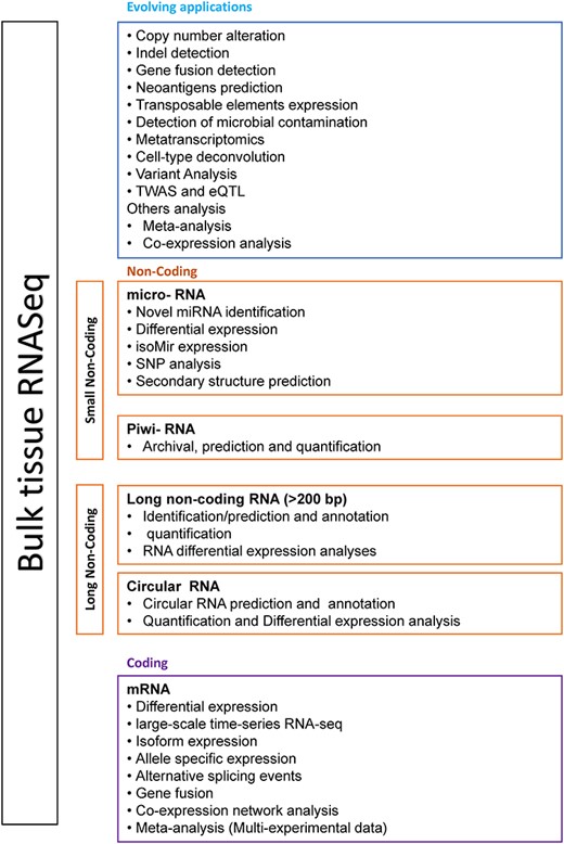
Computational analyses based on bulk RNA-Seq. Core analyses such as transcriptome profiling, differential gene expression, and functional profiling of messenger RNA (mRNA) and microRNA (miRNA) are standard practices. However, Piwi and circular RNA-related studies are still growing from the last few years. Advanced analyses include copy number alteration, indel detections and microbial contamination investigation in RNA-Seq experiments. Other data integration and network analyses to study gene regulatory networks are quite helpful (refer to Supplementary Data).
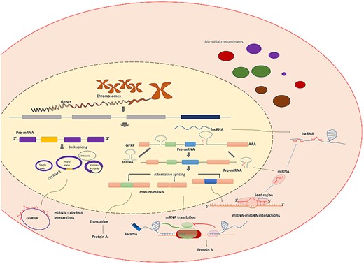
Overview of transcriptomics products and biomolecules interaction. Figure shows a variety of transcriptomics products and the role of various biomolecules interactions in the regulation of gene functionality.
Transcriptome assembly
Typical RNA-Seq applications on common species (such as human or mouse) utilize reference-based methods to map RNA-Seq reads onto a pre-existing reference genome. STAR [16] and HISAT2 [17] are the popular assemblers used for reference-based assembly.
A high-quality genome is available for limited species; therefore, studying rare or new species with RNA-Seq is more challenging and requires the transcriptome of these organisms to be reconstructed through the assembly process [18, 19].
Two different strategies are used for the transcriptome assembly of new species, genome-guided (when the reference genome exists) and de novo assembly. Genome-guided assemblers utilize pre-existing close-related genomes to guide the reconstruction of an alternative consensus sequence. Assemblers map RNA-Seq reads to the reference to orient sequences of new species along the chromosomes. These assemblies are somewhat biased because of their dependence on related reference, and it increases when the transcriptome of a novel organism is not close to the chosen reference [19]. De novo assembly methods, on the other hand, assemble sequences directly from the reads, which is less biased towards using the reference genome, but may be biased towards specific tissue type and conditions from which a sample of a novel species has been sequenced. However, the bias caused by the dependence on a related reference alone can be address by merging de novo and a related reference assembly in contigs [20].
Ungaro et al. [18] compares the reads mapping of the genome of various organisms, using both the transcriptome-guided assembly and de novo assembly; they choose to use a range of different reference genomes having a divergence of >15% from the species of interest. The guided assembly outperforms de novo approach alone, including when the divergence level is high. Holzer et al. [21] compared 10 de novo assembler on nine RNA-Seq datasets spanning different kingdoms of life. Evaluations of the tools is measured in a combination of 20 biological-based and reference-free metrics such as mapping rate, mismatches, reference coverage, contig F1, KC score, etc. Based on summarized metric of 20, the Trinity [22], SPAdes [23] and Trans-ABySS [24], followed by Bridger [25] and SOAPdenovo-Trans [26], generally outperformed the other tools. However, these performances vary among species. The selection of best assembly remains a challenging task, such metrics needs additional factors to be compared, such as tools abilities to reconstruct alternatively spliced transcripts/isoforms. Another example of computational difficulties in assembly is to distinguish the back-splice junctions that arise from an internal tandem duplication (generate duplicate exons within a gene) and the ones used for inferring circular RNA, because these kinds of reads are identical [27].
Evolving applications of bulk RNA-Seq
Copy Number Alteration from bulk RNA-Seq
CNA analyses are commonly used in cancer research. Amplification and deletion of the genes have signalling pathway implications and are a key determinant of molecular dysfunction in oncology. For example, PIK3CA amplification and deletion of the CDKN2A are associated with head and neck squamous cell carcinoma [28]. Many challenges lie in calling the CNA from RNA-Seq data, because of the differences in gene expression, which lead to the read depth variance of different magnitudes across genes. Because of these difficulties, most of these analyses are usually done using whole genome sequencing / whole exome sequencing (WGS/WES). However, recent advancements in bioinformatic tools and methods have assisted in the determination of CNA from bulk and single-cell RNA-Seq (scRNA-seq) data. Some of bulk RNA-Seq-based tools are CaSpER [29], CNAPE [30], CNVkit-RNA [31] and SuperFreq [32].
CNAPE is a machine learning approach that uses prior knowledge from The Cancer Genome Atlas (TCGA) data to predict the CNA in human cancer [33]. CaSpER first utilizes multiscale smoothing of expression signal by five-state Hidden Markov Model. Later smoothing of B allele frequency (BAF) signal is performed, followed by identification of the BAF shift threshold using the Gaussian mixture model. Finally, Copy Number Variants (CNV) correction is done by using the BAF shifts. CaSpER works on both bulk and scRNA-seq data. SuperFreq was initially developed for tracking somatic mutations in cancer. It was recently updated for calling absolute allele-sensitive CNA and can establish the relationship between CNA profile and mutation load in cancer. SuperFreq claims to accommodate small number of samples, paired with normal tumour comparisons. Compared with CNVkit-RNA, SuperFreq provides absolute, allele-sensitive and subclone aware CNA calls. There is no universal definition exists of what magnitude of amplification/deletion should be considered as amplified and deleted gene. For example, as per cosmic (https://cancer.sanger.ac.uk/cosmic/analyses), the gain/amplification of the gene is when the copy number is >5 (ploidy ≤2.7) or >9 (ploidy >2.7); however, the PURPLE [34] definition is 3*sample ploidy for gain/amplification. Furthermore, the significance of CNA of genes is defined based on defined amplification/deletion and its occurrence across samples. Moreover, because of a single copy of sex chromosomes in male, the user should be careful of the threshold for chromosome Y and chromosome X.
Indel detection from RNA-Seq
Small genetic variations, either insertions or deletions, measuring from 1 to 10 000 base pairs in length, are called indels. They can be coding and non-coding, and in coding genome, indels are either frameshift or non-frameshifts. Indels are known to have various functions, such as in cancer, they disable tumour suppression, activate oncogenes and trigger an increased abundance of neoantigens [34]. Indels are less common in the genome than SNVs [35]. It is challenging to identify indels from RNA-Seq because of RNA-Seq library and mapping artefacts (often related to the misalignment of spliced reads). Furthermore, complications arise when somatic indels should be distinguished from germline indels, e.g. in cancer studies, lack of normal/healthy tissue RNA-Seq data presents challenges for the detection of indels from tumour RNA-Seq. New tools such as RNAIndel [36] can handle this three-class classification problem using supervised learning and classify coding indels into somatic, germline and artefacts. Sun et al. [37] demonstrated that RNA-Seq alignment is the most important step for accurate indel identification. In a benchmarked study of indel detection, Slosarek et al. [38] suggested the use of additional filtering using Opossum [39]. Some recent studies recommend the integration of RNA- and DNA-Seq data, which improves the sensitivity for identifying mid-sized and large indels missed by DNA-Seq [40]. For the annotation of indel and CNA tools such as Anntool [41] are in common use.
Gene fusion detection
Gene fusions result from break points combining within previous disparate coding regions and lead to unpredictable and potentially deleterious effects. Such fusions can produce greater amounts of active abnormal protein than non-fusion genes, which could lead to tumour genesis [42]. In cancer, gene fusion has been described with the combination of oncogenes, e.g. recurrent gene fusion is reported between Transmembrane protease, serine 2 (TMPRSS2) and Erythroblast Transformation Specific (ETS) transcription factor genes in prostate cancer [43].
Various tools detect gene fusions from RNA-Seq data based on either read mapping or de novo fusion transcript assembly. After benchmarking 23 different gene fusion detection methods (that leverage RNA-Seq solely as input) on simulated and real RNA-Seq data, Haas et al. [44] concluded that Arriba [45, 46], STAR-Fusion [44] and STAR-SEQR [44] are the most accurate and fastest for fusion detection. New databases and bioinformatics resources can characterize and evaluate the significance of the gene fusion [47]. ChiTaRS 2.1 [48], FusionCancer [49], the TCGA Fusion Portal [50] and FARE-CAFE [51] are the latest gene fusion databases. The ChiTaRS 2.1 database is the largest fusion database that catalogues over 29 000 fusion transcripts, primarily from humans.
Neoantigen prediction from RNA-Seq data
Different genetic events such as Indel, gene fusion, SNV can generate mutant peptides called neoantigens. These neoantigens play a vital role in tumour-specific T cell-mediated antitumour immune response and have applications in immunotherapy [52]. Not only genetic events but alternative splicing also has proven to contribute to candidate neoantigens’ generation [53], but most of the tools use indels, SNVs or gene fusions events for neoantigen prediction. Few tools such as ASNEO [54] identify personalized alternative splicing-based neoantigens from RNA-Seq. INTEGRATE-neo [55] and ScanNeo [56] pipelines have been designed to predict neoepitopes derived from gene fusion and indels, respectively.
Measuring the expression of TEs using RNA-Seq data
TEs are sequences of DNA, which switches location within a genome. These TE elements constitute ~66–69% of the human [57, 58] and 30% fruit fly (Drosophila melanogaster) genomes [59]. They are integrated into a different genomic location either using DNA (‘transposons’) or through reverse transcription (‘retrotransposons’) [60]. There are three types of retrotransposons: long terminal repeats, long intersected elements and short intersected elements (SINEs) [61]. TEs can contribute to the formation of transcription factors [62] and abnormal expression of TE associated with cancer [63], and neurodegenerative diseases [64].
Next-generation sequencing (NGS) has advantages over in vitro techniques for studying retrotransposition, e.g. NGS can detect novel SINE amplification events during development, and this is not possible with in vitro methods. Despite the challenge posed by the repetitive nature of retroelements for developing bioinformatics analyses algorithms, reasonable progress has been made recently by the bioinformatics community. Moreover, in SINE elements, the short length of SINE elements contributes additional difficulty to the identification of the SINE instances that regulate cell functions.
MMR [65] and SalmonTE [66] tools were designed to investigate transposon expression using RNA-Seq explicitly. These packages perform quantification at the subfamily level. However, newer packages SINEsFIND [67] and ERVmap [68] address the need for locus-specific quantification of TE-derived transcripts. Novel fusion events that connect TE promoter sequences to downstream coding gene sequences can also be detected using the LIONS tool [69]. Table 1 describes more TE tools designed for RNA-Seq. For detailed algorithmic strategies, we recommended following TE tools-specific reviews [70–73].
The table lists tools and pipelines for the measurements and analysis of the transposable elements from RNA-Seq data
| Pipeline | Year | Applications or functional use |
|---|---|---|
| GeneTEFlow [9] | 2020 | A Nextflow-based pipeline for analysing gene and transposable elements expression from RNA-Seq data |
| SQuIRE [95] | 2019 | Quantifying interspersed repeat expression (SQuIRE): RNA-Seq analysis pipeline that provides a quantitative and locus-specific picture of TE expression |
| L1EM [96] | 2020 | For accurate locus-specific LINE-1 RNA quantification |
| repEnrich [97] | 2014 | To study genome-wide transcriptional regulation of repetitive elements, the original study shows transcriptionally active long terminal repeat retrotransposon |
| TEtools [98] | 2017 | Facilitates big data expression analysis of transposable elements and reveals an antagonism between their activity and that of piRNA genes |
| TEtranscripts [99] | 2015 | For including transposable elements in differential expression analysis of RNA-Seq datasets |
Detection of microbial contaminants
Advanced tools can detect the contaminants’ presence in the experiment using the same RNA-Seq data, which is sequenced for testing some biological hypothesis. Generally, these tools extract the contaminants information from unmapped reads to the reference genome, i.e. reads that does not map to the reference genome. Many experimental standards have been developed to reduce laboratory contamination, despite this unexpected microbial contamination is reported in many studies. Recent studies [74, 75] suggest that researchers should consider measuring the functional impacts of contamination as this affects the quality of the research. Since cell manipulation for a range of experimental designs is essential in modern research and eukaryotic cells are highly likely exposed to microorganisms at the time of transition. Sometimes these contaminations contribute to a false experimental interpretation because contaminants may cause their host cells to have significant morphological and physiological changes. Furthermore, identifying infectious agents is vital in donated cells in medical and clinical facilities to prevent donor–patient disease transmission. These studies explore the effect of cross-contamination caused by exogenous sources, including laboratory reagents.
Some tools designed for this purpose require full FASTQ files as an input, whereas other new tools work directly on unmapped BAM files. A few tools are explicitly designed for virus detection. VirTect [76], VIRTUS [77] and ViGen [78] detect viruses using RNA-Seq. In contrast, the Decontaminer tool [8] and contamination screen are designed for bacteria, fungal and virus contamination detection. Decontaminer also provides an online visualization architect to explore the experimental contamination in detail.
Metatranscriptomics analysis
Metatranscriptome denotes the total RNA copies of the genes in a community of organisms. At a specific time of sampling, it is considered as a unique entity. Metatranscriptome varies with time and environmental changes. It can be used to obtain the whole expression profile in a community and demonstrate the dynamics of gene expression patterns over time. RNA-Seq is on the rise to conduct metatranscriptomics and microbiome dynamics studies. Metatranscriptomics analysis remarkably studied the alteration of gut microflora and its association with diseases like inflammatory bowel disease [79], obesity [80] and diabetes [81]. The gut microbiome plays roles in directing the host immune system development, post-embryonic development, host behaviour, detoxification [82]. Peters et al. [83] showed a relationship between gut microbiota and immunotherapy responses via metatranscriptomics in melanoma patients. Recently, metatranscriptomics employed as a surveillance tool for detecting the presence of the severe acute respiratory syndrome coronavirus 2 genome through the nasopharyngeal swabs of COVID-19 disease patients [84]. Studies have also explored the microbiome’s role in host evolution [85], which are predicted to be co-evolved [86].
Numerous bioinformatics pipelines are available for metatranscriptomics to investigate complex microorganism communities. These pipelines can be classified as assembly-free and assembly-based pipelines [87]. HUMAnN2 [88], MetaTrans [89], SAMSA2 [90] use assembly free strategy. SqueezeMeta [91], IMP [92] and MOSCA [93] are assembly-based tools. MetaTrans and SAMSA2 implemented for both taxonomic and differential gene expression analysis purposes, whereas HUMAnN2 does not carry out differential gene expression analysis. Among assembly-based tools, only MOSCA performs differential expression (DE) studies; the rest two, SqueezeMeta and IMP, are limited to taxonomic and functional analysis. Galaxy-based pipeline, ASaiM-MT [94], is designed for functional and taxonomy quantitation using HUMAnN2 and MetaPhlan2, respectively. The accurate quantification of organisms or functional activity within the complex metatranscriptome of samples remains an open challenge, because it is difficult to identify the optimal sampling frequency for different times, and the compositional nature of microbiome data frequently violates assumptions of statistical methods.
Determining cell type abundance (cell type deconvolution) and expression from bulk tissues
The method of estimating the proportion of each cell type is called cell type deconvolution, which is essentially performed with cell type-specific gene expression profiles for bulk transcriptomics samples [100]. Understanding the composition of cell types in disease-relevant tissues is an important step towards discovering cellular disease targets. Flow cytometry or single-cell RNA-Seq are most commonly used for cell type deconvolution. Currently, advanced bioinformatics tools can perform the same task using bulk RNA-Seq, which also estimates cell type abundances. For example, CIBERSORTx [101] tool can infer cell type-specific gene expression profiles without physical cell isolation using machine learning models, and its utility is evaluated in several types of tumours. In Table 4, we list the cell type deconvolution tools for bulk RNA-Seq and highlight the essential features for each. These tools can be used to define the cellular heterogeneity of complex tissues such as cancer to investigate the mechanism of disease.
Variants calling from RNA-Seq
SNVs offer insights to decipher the novel biological mechanisms for complex diseases and define genotype and phenotype associations. The genomic and genetic variation provides clues to the drivers of both malignancy and metastasis [101–103]. The variant identification can be statistically challenging due to low sequencing depth and lower variant allele frequency. Diseases such as cancer further increase these challenges because of tumour subpopulation, low tumour purity or a highly disturbed genome. Typically, whole-genome/exome sequencing is predominantly used for calling genomics variants rather than transcriptome (RNA-Seq). However, the relatively lower cost of RNA-Seq is gaining attention as an alternative to Whole Genome sequencing/ Whole exome sequencing (WGS/WES). Even though variant calling from RNA-Seq has drawbacks, it can help in the investigation of discrepancies at both the transcriptomic and genomic level due to post-transcriptional modifications. For example, RNA editing, nonsense-mediated decay, could be missed in genomic data. Conversely, RNA-based variant calling can miss (a) variants in the alleles, which are not expressed, (b) splicing variants, (c) variants in the low-expressed gene and (d) is limited to expressed region, etc. In conclusion, both methods have pros and cons. Wherever applicable, integration of both is the best solution for exploring the genotypic and phenotypic relationship; for example, Coudray et al. [104] shows in the absence of RNA-Seq data, WES/WGS likely to miss key driver mutations [105].
The important variant calling pipeline steps are mapping, marking the duplicates, base recalibration, variants calling, filtering of low-quality variants and variants annotations. Identification of genomic variants from RNA-Seq data is further complicated by intrinsic complexity such as splicing, low-expressed regions and managing duplicate reads, but algorithms are evolving day-by-day. Many variants calling pipelines have been developed for underlying models, filters, input data requirements and targeted applications. These pipelines generally use different variant callers for calling germline and somatic variants. Table 2 details variant calling pipelines dedicated to RNA-Seq data.
RNA-Seq-based variant calling pipelines. Various pipelines commonly used for variant calling from RNA-Seq data are reported in the table with the information of the aligner and variant caller used in the pipeline
| Pipeline | Year | Aligner or input | Variant caller |
|---|---|---|---|
| Opossum + Platypus [39] | 2017 | Opossum pre-processes BAM (TopHat2 or Star 2-pass) | Platypus or GATK HaplotypeCaller |
| STAR 2-pass + MuTect2 [104] | 2018 | STAR 2-pass | MuTect2 |
| VAP (Variant analysis Pipeline) [113] | 2019 | Star 2-Pass | GATK Haplotypecaller |
Earlier tools based on non-splice aware aligners contribute little to address false positives calls due to the transcriptome complexity. To overcome these limitations, modern pipelines such as VAP work with a splice-aware aligner (e.g. STAR [16]) and use transcripts annotation data to identify reliable SNPs in RNA-Seq. Further prioritization of RNA variants can be done with tools such as RVboost. RVboost uses a boosting technique to train a model of ‘high-quality’ variants by using common HapMap variants, and RNA variants are prioritized and called on the basis of the trained model. Another machine learning tool ‘SmartRNASeqCaller’ [106] has been developed to improve true germline variants and minimize the burden of false-positive calls from RNA-Seq. ANNOVAR [107] and Ensembl Variant Effect Predictor [108] are top-rated tools for the annotation of the variants called by variant callers. However, new platforms such as open-cravat [109] provide varieties of tools for annotating variants as per user needs. Radenbaugh et al. [110] reported that inclusion of the RNA-Seq with genomic data increases the power to detect somatic mutations.
Identifying the cancer malignancy driver genes is quite challenging, because a high mutation rate in cancer often introduces random mutations everywhere in the genome. Highly mutable genes are not simply driver’s genes, as it is often assumed that genome-wide mutation rate is constant, e.g. mutation rate for lowly expressed and late replication genes is usually higher. Moreover, higher gene length contributes towards a false-positive signal for a driver gene. Whole exome sequencing (WXS)/WES approaches-based tools like MutsigCV [111] and OncodriveFML [112] deal with such biases and help to predict the positive driver signals. As per our knowledge, currently, similar tools are not developed for RNA-Seq-based data.
Expression quantitative trait loci and transcriptome-wide association study analysis
The genome-wide association studies (GWAS) link the association between the gene variations (SNPs) and the complex phenotype/disease. However, GWAS approaches are unable to find the causal SNPs or in vitro confirmation to interpret biological functionality. GWAS also ignored the association between genetic variants, DNA functional elements and complicated traits and diseases. Expression quantitative trait loci (eQTL) studies can help identify the extent of influence that a variant can have on gene expression. eQTL are the genetic variants associated with the expression levels of one or more genes located near a variant (cis-eQTLs) or in a distant location from the variant (trans-eQTLs). A typical eQTL analysis is based on statistical hypothesis testing between SNP genotypes and gene expression levels are result in P-values that represent the strength of the association between the two measurements. Since trans-eQTL identification involves many more genes to be tested, the eQTL association to the distant genes remains challenging. In the same study subjects, the importance of gene expression regulation proved by eQTL studies by measuring both genetic variation and transcriptome data. However, these designs are not cost effective. Because of the complicated extraction procedure and other clinical reasons, for some trait, usually, a limited number of datasets with matched GWAS and transcriptome data are available. Limited sample size does not provide enough power for the analysis. When transcriptome data are not available in GWAS samples, transcriptome-wide association study (TWAS) offers novel insights into complex disease mechanisms [114]. TWAS emerged as a powerful approach that integrates common features of eQTL and GWAS studies (generally utilize different population-based data) to test the gene–trait associations and prioritize potential causal genes having the effects of a mediate variant on the traits. TWAS helped in discovering this relationship with improved statistical power and reduced multiple testing burden (i.e. number of genes) compared with testing traits with genetic variations (i.e. number of SNPs) [115]. TWAS is a robust framework to discover susceptible risk genes in complex human traits [116]. TWAS determines if GWAS-significant variants are also enriched for eQTLs by detecting co-localization of expression signals at known GWAS loci [117].
For eQTL analysis, tools use various strategies such as one-at-a-time test (Krux [118], MatrixeQTL [119], GeneVar [120]), multiple regression (HEFT [121]) and one-at-a-time-regression (SNPTEST [122], R/QTL [123]). When an intricate linkage disequilibrium structure is present, the one-at-a-time strategy cannot control the false positives. Also, this approach is often underpowered to detect the full spectrum of trans-acting regulatory effects. Other tools based on Bayesian statistics are Sherlock [124], eQTLBMA [125], etc. Multivariate eQTL mapping approaches, either least absolute shrinkage and selection operator (LASSO) or Bayesian Evolutionary Stochastic Search (ESS), are more suitable for detecting polygenic effects [126]. Furthermore, many TWAS integration and analysis methods have been published in the recent past, such as PrediXcan, which constructs a weighted SNP-set-based test in GWAS using SNP weights directed from the expression mapping studies [117]. Another method, TWAS, predicts the association between the complex phenotype/disease and the predicted quantitative gene expression built using the Bayesian sparse linear mixed model [127]. To incorporate the randomness and to deal with complexity in the polygenic architecture of expression data, a non-parametric latent Dirichlet process regression (DPR) model was incorporated for TWAS [128]. Similarly, TIGAR is also DPR model based, but provides a user-friendly interface. Other tools are developed on Mendelian randomization and perform tests to predict the causal relationship between gene expression and disease trait; these are summary data-based Mendelian randomization (SMR) [129] and Generalized SMR (GSMR) [130], respectively. In conclusion, TWAS can facilitate our understanding of the molecular and causal mechanisms underlying variant–trait associations. TWAS developed a few years ago, and since then, it helped into the GWAS-prioritized SNPs, which may have a crucial role in revealing the cis-SNPs regulating the upstream target gene. Moreover, eQTL analysis is not limited to the coding part, but it is also used for various non coding RNAs (ncRNAs), such as long non-coding RNA (IncR)-eQTLs, miRNA QTLs and circular RNA (circRNA)-eQTLs, etc. eQTL mapping can be performed based on tissue types as well. However, much work is still required to elucidate the effect of trans-SNPs on the neighbouring upstream target gene of interest and the effect of rare variants.
mRNA-related analyses and application
One of the primary motives of most RNA-Seq studies is DE analysis between two or multiple conditions or comparing different phenotypes.
Differential expression analysis
DE analysis of RNA-Seq compares the transcriptomic expression of different diseases’ phenotypes or conditions and measures unknown transcripts that other old techniques such as microarray were not capable of detecting. Because of its low cost, it became a popular choice in various research applications, including the discovery of potential biomarkers and therapeutic targets in cancer [131].
Regardless of the type of the study, to access transcriptomic differences using read counts, one has to first map reads to the reference genome and quantify them. The quantification of reads depends on various transcriptomics features that one wants to measure i.e. genes, exons or gene isoforms. After reads are quantified, few steps are recommended before performing downstream DE analysis, such as filtering lowly expressed genes, normalization and/or batch effect correction. Filtering is recommended to eliminate low abundant genes that are believed to contribute to false discovery rate. Normalization (although not always required) corrects counts for various technical factors, including sequencing depth, RNA composition or gene length. The most common normalization techniques are Fragments Per Kilobase of transcript per Million mapped reads (FPKM), Reads Per Kilobase of transcript per Million mapped reads (RPKM), Counts Per Million (CPM), Trimmed Mean of M-values (TMM) and median of ratios. Depending on the design of the experiment, RNA-Seq data may also suffer from various systematic biases that can affect downstream analysis results. To remove unwanted variation in RNA-Seq data, one can apply methods like ComBat [132] or RUV-Seq [133]. Different complex statistical models are used to test which features have significant differences in their counts between the conditions. These models are often based on various data distribution assumptions, including negative binomial (NB) in DESeq2 [134], edgeR [135], or EBSeq [136], log-normal distribution in Ballgown [137], or relaxing the assumption of any distribution (non-parametric) as in NOISeq [138]. In case of high variabilities of gene expression within a condition or phenotype, a higher number of biological replicates are preferred to get significant statistical power in detecting differentially expressed features. Depending on the biological question to answer, comparison between the conditions can be performed in various forms such as pairwise, multiconditional or time series. To date, several reviews and studies have been published for the guidelines and best practices of the RNA-Seq applications [139, 140].
Large-scale time series RNA-Seq
Typically, static RNA-Seq captures a snapshot of the transcriptome at the time of sample collection, whereas the time series RNA-Seq methods are applications of RNA-Seq, which measures RNA abundances over time in biological samples. Its applications include the exploration of cellular differentiation, developmental biology processes, disease progression, etc. The general aim is to identify specific gene expression pattern over time. However, statistical analysis of time course data is challenging because of complex experimental design, large dynamic changes of the transcriptome. Compared with static RNA-Seq methods, these methods are not well benchmarked and validated [139]. Recent reports inform that no comparative study compares these tools considering metrics of factors such as the impact of pre-processing steps, various time points, different numbers of replicates, multiple conditions and variable noise levels. Table 3 explain various tools based on time course analysis. Each tool has its pros and cons, and at the individual level, no pipeline can address the complete characterization of the dynamic biological process. Tools based on static RNA-Seq have a major assumption that observed samples are collected independently at a fixed time point; hence, not appropriate for time course RNA-Seq statistic.
Large-scale time series RNA-Seq analysis tools
| Software | Year | Applications feature |
|---|---|---|
| MAPTest [161] | 2020 | Two series time course; longitudinal settings in repeatedly measured data; also enables classification between parallel differential expression or non-parallel differential expression |
| deepTS [162] | 2020 | Flexible and powerful web-based platform for identification and analysis of pairwise transcriptome data along with the visualization |
| AR (auto-regressive model) [163] | 2019 | Single series of longitudinal RNA-Seq time course data; balanced longitudinal data required with an even number of sample size; longer running time required as number of time point increases |
| ImpulseDE2 [164] | 2018 | One- or two-series time course data, longitudinally measured RNA-Seq and Chip-Seq data with more than six time points |
| Trendy [165] | 2018 | Single-series time course; longitudinally measured, use optimal segmented regression model; provides the location and direction of dynamic changes in expression |
| TSIS [166] | 2017 | Detects transcript isoform switches, graphic interface performed by Shiny app from R package |
| timeSeq [167] | 2016 | Two-series time course; method based on negative binomial mixed-effects model with major factors; distinguish non-parallel versus parallel temporal changes between conditions over time |
| EBSeq-HMM [168] | 2015 | Single-series time course; longitudinally measured, use auto-regressive Hidden Markov Model |
| Ngsp [169] | 2015 | One- or two-series time course; longitudinally measured, and advantageous for temporal dynamic patterns incorporated course experimental designs |
| Next maSigPro [170] | 2014 | One- or multi-series time course data; non-longitudinally measured, and use polynomial regression model for a different time variable. DEG is selected by the best-fitted model in a temporal manner |
Tools and pipelines for cell type abundance measurement from bulk tissue
| Tool | Year | Features | Programming language | Software link |
|---|---|---|---|---|
| TIMER2.0 [193] | 2020 | Web server for comprehensive analysis of tumour-infiltrating immune cells | Web-tool R, Javascript | https://github.com/taiwenli/TIMER |
| CIBERSORTx [101] | 2019 | Impute gene expression profiles and provide an estimation of the abundances of member cell types in a mixed cell population | Web-tool Java, R | https://cibersortx.stanford.edu/ |
| quanTIseq [194] | 2019 | Quantify the fractions of 10 immune cell types from bulk RNA-sequencing data | R, Shell (Bash) | https://icbi.imed.ac.at/quantiseq |
| Immunedeconv [12] | 2019 | Benchmarking of transcriptome-based cell type quantification methods for immune oncology | R | https://github.com/icbilab/immunedeconv |
| Linseed [195] | 2019 | Deconvolution of cellular mixtures based on linearity of transcriptional signatures | C++, R | https://github.com/ctlab/LinSeed |
| deconvSEQ [196] | 2019 | Deconvolution of cell mixture distribution based on a generalized linear model | R | https://github.com/rosedu1/deconvSeq |
| CDSeq [197] | 2019 | Simultaneously estimate both cell type proportions and cell type-specific expression profiles | MATLAB, R | https://github.com/kkan g7/CDSeq_R_Package |
| dtangle [198] | 2019 | Estimates cell type proportions using publicly available, often cross-platform, and reference data | R | https://github.com/gjhunt/dtangle |
| GEDIT [199] | 2019 | Estimate cell type abundances | Web-based tool Python, R | http://webtools.mcdb.ucla.edu/ |
| EPIC [200] | 2017 | Simultaneously estimates the fraction of cancer and immune cell types | R | http://epic.gfellerlab.org/ |
| WSCUnmix [201] | 2017 | Automated deconvolution of structured mixtures | MATLAB | https://github.com/tedro man/WSCUnmix |
| Infino [202] | 2017 | Deconvolves bulk RNA-Seq into cell type abundances and captures gene expression variability in a Bayesian model to measure deconvolution uncertainty | R, Python | https://github.com/ham merlab/infino |
| MCPcounter [203] | 2016 | Estimating the population abundance of tissue-infiltrating immune and stromal cell populations | R | https://github.com/ebec ht/MCPcounter |
Allele-specific expression
The diploid genome with two paternal alleles of a gene has a relative difference in the allelic transcription due to various factors, viz differential rates of transcription, relative differences in the mRNA stability and multiple cis- trans-regulatory elements in action to control the allelic transcription abundance. These allelic expression differences can range from a slight quantitative change to many folds up/down in magnitude [141–143]. Thus, accurate estimation of the differential abundance of a gene’s allelic copies is referred to as allele-specific expression (ASE). It provides a substantial understanding of alleles’ relative expression in a diseased state termed as eQTLs [144, 145]. RNA-Seq can measure the ASE of the gene coming from parental alleles. Usually, the heterozygous SNP information in the transcribed genomic region helps differentiate the RNA-Seq reads’ origin. The paternal and maternal allele gene expression ratio is used to measure the ASE differences, which may lead to some phenotypic variations. RNA-Seq analysis platforms have grown robust and sensitive enough to provide quantitative information on differential ASE for genes [142, 143].
The standard reference-based mapping approaches suffer from the biased estimation in favour of the most abundant allelic counterpart matching with the reference genome or transcriptome [144, 146]—many attempts to circumvent this bias while scoring the alignment [145, 147, 148]. Among many approaches, one of the chief steps involved was hashing method, which refers to assigning reads to the alleles with the already known SNP [149]. WASP tools are based on this approach [150] and speculated that approach helped in navigating the fact that SNPs matching to non-reference transcripts usually match to multiple genomic locus. Thus, allele assignment of these reads is discarded in WASP. Another tool, ASElux, assigns SNPs, quantifies allelic reads directly from unmapped RNA-Seq datasets [151]. Some tools developed using statistical approaches to deal with the individual-specific random effects to assign SNPs using multi-SNP correlations for a single transcript. ASE analysis in a population tool intakes RNA-Seq datasets and infers multi-SNPs correlations for a single gene-level ASE between two conditions [152]. The other tools in this related domain using statistical approaches are GeneiASE [153], QuASAR [154] and MBASED [155]. In addition, a set of best practices, comprehensive discussion on the ASE expression methods from RNA-Seq datasets is provided here [156].
Differential isoform expression and differential splicing
Recent transcriptome analyses have shown that up to 95% of human genes are alternatively spliced to encode proteins with different functions [157]. There are two types of splicing described: (1) constitutive splicing and (2) alternative splicing. In constitutive splicing, non-coding introns are removed from the pre-mRNA, and exons are joined together to form a mature mRNA [158, 159], whereas in alternative splicing, exons can be included or excluded in different combinations to create a diverse range of mRNA transcripts from a single pre-mRNA. It serves as one of the major mechanisms to increase the diversity of the transcriptome. Alternative splicing events are commonly classified into various categories such as cassette exons, mutually exclusive exons, retained intron, alternative 5′ splice sites, alternative 3′ splice sites, alternative promoters and alternative poly-A sites [160]. In a cassette exon, an intervening exon between two other exons from the mature mRNA sequence can be either included or skipped to generate two distinct protein isoforms. In the case of intron retention, the intron removal can be suppressed, resulting in the entire intron’s retention. Alternate splice sites of 5 ‘or 3’ can extend or shorten the exons. Intron retention is generally the most difficult type to detect due to the experimental artefacts. Since incompletely spliced transcripts may retain the intron fragments, which can be mislabelled as the intron’s retention.
Identification and analysis of alternative splicing events
The advancement of RNA-Seq methods has facilitated the study of the splicing process’s genome-wide impact and regulation. New bioinformatics tools led to the identification of novel transcribed regions and splicing isoforms and provided that a significant fraction of the transcribed RNA in human cells undergo alternative splicing [171]. An increasing number of studies illustrated that the selection of wrong splice sites causes human disease [172], emphasizing the importance of studying differentially spliced transcripts. However, the large datasets produced from RNA-Seq experiments and complex information to analyse have turned this into a challenging task.
Several tools have been developed for quantification and identification of alternative splicing events such as SpliceR [173], SpliceSeq [174], splicing Viewer [175], ASTALAVISTA [176, 177], GESS [178], DiffSplice [179], DSGseq [180], GLiMMPS [181], GPSeq [182], MATS [183], rMATS [184], MISO [185], JuncBASE [186], finesplice [187], SpliceTrap [188] and ASpli2 [189]. Each tool has its advantages and disadvantages. In the context of alternative splicing, the SpliceSeq, SpliceViewer, DiffSplice and ASTALAVISTA tools also facilitate intuitive visualization of RNA-Seq results. GESS (graph-based exon-skipping scanner) performs de novo detection of skipping event sites from raw RNA-Seq reads without prior knowledge of gene annotations. GESS method builds a splice site-link graph from first hand, raw RNA-Seq reads and then implements a walking strategy on this graph by iteratively navigating subgraphs to reveal those with a pattern corresponding to an exon-skipping event. Thus, it can provide a more accurate and comprehensive picture of skipping events associated with a cell’s particular physiological condition.
Both GESS and DiffSplice can identify splicing events without prior annotation. MATS compares two samples without replicates, whereas rMATS compares two samples with replicates. Running rMATS without replicates automatically invokes the MATS algorithm. DSGseq is an exon-based method that uses the NB distribution to model sequencing reads on exons and proposes an NB-statistic to detect differentially spliced genes. It can also detect the novel alternative splicing events and highlight differentially spliced.
MISO (mixture-of-isoforms) model is a statistical model that estimates the expression of alternatively spliced exons and isoforms and assesses confidence in these estimates from RNA-Seq data. The MISO model uses Bayesian inference to compute the probability that a read originated from a particular isoform. ASpli evaluate the difference in AS events’ magnitude by comparing the exon inclusion or intron retention percentage using splice junctions, and for the differential use of introns, exons and splicing junctions, read counts are used. This integrative process enables to detect the differences in both annotated and novel AS events. Main steps involved in the ASpli workflow are parsing the genome annotation into bins and aligning the read against the bins. Finally, based on the count of the reads aligned to the bins or junction, differential bins are inferred.
To identify alternative splicing events, SpliceR utilizes the full-length transcript output from RNA-Seq assemblers. SpliceR also annotates the differentially spliced elements’ genomic coordinates, facilitating downstream sequence analysis of each splicing pattern. Fraction values are calculated for each transcript isoform to detect the transcript switching between conditions. MISO, ASTALAVISTA and DiffSplice are unable to evaluate novel features because these methods do not generate the genomic coordinates of differentially spliced regions. Recently various approaches for differential splicing and DE at isoform have been benchmarked [190] and reviewed [191, 192], highlighting basic characteristics along with the pros and cons of some of the commonly used software.
Prospective
RNA-Seq algorithms and methodologies are continuing to evolve. Advancement in statistical models vastly improved bioinformatics methods, and many new applications of the RNA-Seq-based analyses are now possible. The key statistical considerations and methods evolved at sample level, gene/transcript level, exon level and the methods diversified with respect to different statistical models and data distributional assumptions. As the novel tools are now providing various ways to answer the same biological question, the pitfall for the user is to choose the most optimal and appropriate model. The choice of parameters within the method can also impact the final results and interpretation of data. In that case, it is recommended to try various tools and settings and to support the choice of the model by benchmarking studies and in-depth reviews of the methods. However, the user should carefully design their experiment and optimize the experimental design by power analysis for RNA-Seq beforehand. If biological samples are processed in different batches of the sequencing, the use of technical replicates is also recommended.
Bias due to sequencing library can also alter the outcome, e.g. insufficient small non-coding RNA (sncRNA) detection bias due to RNA modification, isoforms detection bias due to short reads. The new sequencing method PANDORA can detect sncRNAs that once undetected by other libraries due to RNA modification that interferes with ligation and reverse transcription. Similarly, an improved read coverage and sequencing depth can overcome the disadvantage of short read length. New technologies such as long-read sequencing and scRNA-seq open new possibilities where short-read sequencing and bulk RNA-Seq have limitations. For example, long RNA-Seq can better resolve the genome assembly of the highly repetitive region of the larger genomes. Furthermore, it can detect long structural variants, full-length isoforms sequence and examine splicing better than short-read sequencing. On the other hand, scRNA-Seq helps understand tumour heterogeneity and drug-resistant clones with higher resolution. It is also very efficient in the investigation of cell lineages and cancer stem cell evolution. Other NGS and microarray technologies restricted rare cell type analyses to a large cell population only, but scRNA-Seq can analyse rare cell type more efficiently. scRNA-Seq assisted in the identification of exhausted CD8 cells in cancer therapy and establishing drug-resistant clones with higher resolution. Furthermore, with the help of time course scRNA-Seq experiments, we are opening up a wealth of biological information regarding spatio-temporal gene expression at different stages of cell growth or under disease stages. On the other hand, it is not straightforward to construct the cell lineages from the bulk RNA-Seq and microarray-based technologies. In the past, the gene regulatory networks was used to construct time series datasets from bulk and microarray platforms. However, these methods cannot identify the rare cell type and perform downstream analyses in a computationally efficient way.
This review described the evolving methodology for bulk RNA-Seq-based analysis and highlighted the knowledge gaps. Due to different biological aims and scenarios, finding consent on the best tools or pipelines is challenging. However, within the scope of this article, we provided a good summary of methods and information on available resources together with benchmarking studies that can help non-experts users orient themselves on new applications that bulk-RNA-Seq analysis can accommodate.
Detection of genomic features from RNA-Seq data with advanced bioinformatic algorithms.
Evolving bioinformatic tools have the potential to discover more hidden information in bulk RNA-Seq data such as microbial contamination, TEs expression, CNAs, neoantigen prediction and cell type deconvolution, etc.
Exploration of advance TWAS using bulk RNA-Seq.
Funding
The National Health and Medical Research Council Project Grant APP1181179 Ideas Grant (to A.S.T., B.A. and M.R.). Czech Science Foundation (20-04099S to P.K.T.).
Amarinder Singh Thind is a postdoctoral researcher (Bioinformatics) at the University of Wollongong, Australia and IHMRI. His current research interests include the development of methodology for the integration of genomics, coding and non-coding transcriptome to discover biomarkers in cancer contexts.
Isha Monga is working as postdoctoral research scientist at the Department of Dermatology, Columbia University Medical Center, New York. Her research interests include understanding and elucidation of the molecular mechanisms of skin disorders including autoimmune disease alopecia areata. To achieve that, she is currently analysing high-throughput datasets of the single-cell sequencing, GWAS fine-mapping and 3D genomics methods from the mouse model and patients’ skin samples.
Prasoon Kumar Thakur is a Bioinformatician at the laboratory of RNA Biology at the Institute of Molecular genetics, Prague, Czech Republic and pursuing a PhD degree at Charles University, Prague, Czech Republic. The focus of his current research is RNA splicing and high-throughput data analysis.
Pallawi Kumari is a Bioinformatics researcher at IMTECH-Bioinformatics Centre, Chandigarh, India. She has expertise in NGS genomics and transcriptomics. Her research interests lie in human cancer genetics.
Kiran Dindhoria is a research fellow at MTCC, CSIR-IMTech, Chandigarh, India. She has expertise in NGS genomics and metagenomics. Her research interests lie in human microbiome studies.
Monika Krzak is a postdoctoral researcher in Bioinformatics at the Genomics of Inflammation and Immunity Group at Sanger Institute, UK. Her research interests are focused on understanding the pathogenesis of immune-mediated diseases.
Marie Ranson is a Professor of Molecular Biology at the University of Wollongong, Australia. She has longstanding research interests in biomarkers of cancer invasion and metastasis. She has made substantial contributions to the plasminogen activation system field in cancer as well as in inflammatory diseases. She has also successfully led and/or contributed IP to several drug development projects related.
Bruce Ashford is a surgeon scientist within the Medical School, University of Wollongong, Australia. His current research interests include bioinformatics, health informatics, molecular oncology and reconstructive microsurgery. The main focus of his research is to discover biomarkers in cSCC cancer using various omics methods.
References
Youngblut, Nicholas D., Georg H. Reischer, William Walters, Nathalie Schuster, Chris Walzer, Gabrielle Stalder, Ruth E. Ley, and Andreas H. Farnleitner.
Pagel, K.A., Kim, R., Moad, K., Busby, B., Zheng, L., Tokheim, C., Ryan, M. and Karchin, R.
Frazee AC, Pertea G, Jaffe AE, Langmead B, Salzberg SL, Leek JT.
Merino GA, Conesa A, Fernández EA.
