


Abstract
The heating of tungsten monoblocks at the ITER divertor vertical targets is calculated using the heat flux predicted by three-dimensional ion orbit modelling. The monoblocks are beveled to a depth of 0.5 mm in the toroidal direction to provide magnetic shadowing of the poloidal leading edges within the range of specified assembly tolerances, but this increases the magnetic field incidence angle resulting in a reduction of toroidal wetted fraction and concentration of the local heat flux to the unshadowed surfaces. This shaping solution successfully protects the leading edges from inter-ELM heat loads, but at the expense of (1) temperatures on the main loaded surface that could exceed the tungsten recrystallization temperature in the nominal partially detached regime, and (2) melting and loss of margin against critical heat flux during transient loss of detachment control. During ELMs, the risk of monoblock edge melting is found to be greater than the risk of full surface melting on the plasma-wetted zone. Full surface and edge melting will be triggered by uncontrolled ELMs in the burning plasma phase of ITER operation if current models of the likely ELM ion impact energies at the divertor targets are correct. During uncontrolled ELMs in pre-nuclear deuterium or helium plasmas at half the nominal plasma current and magnetic field, full surface melting should be avoided, but edge melting is predicted.
Export citation and abstract BibTeX RIS
Glossary
| CHF | critical heat flux |
| CX | charge exchange |
| ELM | edge localized mode |
| HHF | high heat flux |
| IVT | inner vertical target |
| LE | leading edge |
| MB | monoblock |
| OHS | optical hot spot |
| OVT | outer vertical target |
| PFC | plasma-facing component |
| PFU | plasma-facing unit |
| PG | poloidal gap |
| PIC | particle-in-cell |
| QSPA | quasi-stationary plasma accelerator |
| TG | toroidal gap |
| VT | vertical target |
| W | tungsten |
Symbols which are freqently used throughout this paper (the meaning of standard symbols, such as B for magnetic field, and some symbols that appear punctually in specific Sections and which can be understood by local context, are not defined here)
| α | magnetic field incidence angle with nominal divertor target surface |
| Δθ | tilting angle of divertor targets |
| ΔtELM | time of flight of ELM ions from the H-mode pedestal to the divertor target |
| Δr | radial step between toroidally adjacent MBs |
| ΔT1D | ELM-induced temperature increase of a nominal, axisymmetric divertor target surface |
| εsurf | local ELM energy fluence normal to a real surface |
| εtg | ELM energy fluence normal to an ideal, axisymmetric divertor target |
| ϕ | ion gyrophase angle |
| θ⊥ | magnetic field incidence angle projected on the plane that is perpendicular to the nominal divertor target surface and parallel to the toroidal direction |
| θ// | magnetic field incidence angle projected on the plane that is parallel to the nominal divertor target surface |
| θψ | inclination angle of magnetic flux surfaces with respect to nominal divertor target surface normal vector |
| τd | decay time of an ELM heat pulse |
| τIR | time at which the surface temperature as measured by an infra-red camera attains its maximum value during an ELM |
| τr | rise time of an ELM heat pulse |
| FHF | transient heat flux factor |
| HMB | nominal height of MBs |
| gMB | nominal width of toroidal gap between MBs on a given PFU |
| gPFU | nominal width of poloidal gaps between PFUs |
| htor | depth of MB toroidal bevel |
| LMB | toroidal length of MBs |
| mpol | poloidal misalignment between adjacent MBs on a given PFU |
| mrad | radial misalignment between adjacent MB plasma-facing surfaces |
| mtor | toroidal misalignment between adjacent PFUs |
| q// | plasma heat flux parallel to magnetic field lines |
| qrad | radiant heat flux (carried by photons and CX neutrals) normal to an ideal, axisymmetric divertor target |
| qsurf | local projection of the heat flux normal to a real surface |
| qtg | projection of the heat flux normal to an ideal, axisymmetric divertor target |
| rDT | mean Larmor radius of a 50/50 mix of deuterium and tritium ions |
| spol | surface coordinate running over a MB in the poloidal direction |
| stor | surface coordinate running over a MB in the toroidal direction |
| Tinit | initial MB surface temperature before the onset of an ELM pulse |
| WMB | poloidal width of MBs |
1. Introduction
Surface heat load management in nuclear fusion reactors, whether by design or by active control schemes, in respect of the hard limits imposed by material properties, is a challenge. The ITER tokamak will begin operation with a full tungsten (W) divertor consisting of pure W monoblocks (MB) bonded to CuCrZr water-carrying cooling tubes. The maximum manageable heat loads to the divertor are imposed by engineering knowledge of material and technology limits, and validated by tests in high heat flux (HHF) devices [1]. The elaboration of high-performance operation scenarios that respect these limits is guided by the predicted steady and transient thermal loads that could be delivered by the plasma to the plasma-facing components (PFC), based on the most up-to-date knowledge from both physics modelling and extrapolation from current devices [1–4]. These predictions are continually evolving as a result of code development and improvements in diagnostic methods.
The reference shaping solution for the ITER divertor is the key design feature still to be decided. In order to provide the best possible basis for this choice, there is intense coordinated activity in laboratories around the world to model and measure the behaviour of W under realistic heat loads. From the plasma modelling side, these loads are specified in terms of maximum heat flux qtg normal to an ideal, axisymmetric, unshaped divertor target surface. An example is the peak heat flux to the divertor target calculated on a 2D mesh on a poloidal cross-section by the SOLPS code [5] (designated qpk in that work). At the target side, MB shaping, misalignment, and castellation inevitably lead to local peaking of the surface heat flux, qsurf. This paper aims to contribute analysis which narrows the gap between the predicted poloidal power flow towards the divertor targets, and the detailed heat flux distribution over the fine scale surface features of those targets; that is, for a given qtg arriving at the divertor, to predict the local qsurf distribution over each MB. The findings of this parametric analysis allow risks for the divertor to be assessed subject to the specified plasma physics heat load input and shaping design features.
Work is underway to predict heat flux distributions on MBs comparing three models with increasing degrees of sophistication: the optical (or guiding center) approximation, an ion orbit model neglecting electric fields which is developed in this paper, and particle-in-cell (PIC) simulations [6] including ions and electrons with self-consistent electric fields [7]. The optical approximation has been historically used to design plasma-facing components so as to provide perfect magnetic shadowing of exposed leading edges (LE). The ion orbit model without electric fields predicts that power can reach shadowed surfaces due to finite Larmor radius effects. This paper focuses on optical and ion orbit simulations. Comparison with self-consistent, collisionless PIC simulations is discussed in [8].
The input parameters of the model presented here are outlined in section 2. They include the magnetic field orientation at the inner and outer vertical targets (VT), and the MB geometry and assembly tolerances. The ion orbit model itself is described in section 3. Even though it improves significantly the description of heat loads at gap edges with respect to the optical approximation, the physics of the Debye sheath is missing. Nonetheless, it has been found that the heat load predictions agree quite well with self-consistent PIC calculations including the sheath electric field [8]. Analysis is presented which contributes to explaining why this is so. Typical plasma heat loading at poloidal gaps (PG), toroidal gaps (TG), and at 'optical hot spots' (OHS) are described. Finally, the method for handling radiative heating inside gaps due to photons and energetic neutrals is given.
In HHF ITER qualification tests, MB top surfaces8 are uniformly irradiated using electron beams at near perpendicular incidence with a specified power density. This produces a simpler thermal response than will occur in ITER because of the way power is transported to the divertor targets. In the tokamak, the main contribution to surface heating comes from plasma flow along magnetic field lines which strike the target at glancing angles of incidence, combined with intense irradiation by photons and energetic neutrals emanating from charge exchange (CX) reactions. ITER specifies a maximum value for the peak stationary heat flux of qtg ~ 10 MW m−2 which is defined as being oriented perpendicular to the axisymmetric envelope of the VTs and does not account for local target shaping. It will be shown that the local surface heat flux delivered to the MBs by plasma will be ~50% higher than the plasma component of qtg due to the increased angle of incidence resulting from tilting of the targets and toroidal beveling of the MBs. The resulting surface temperature over much of the MB surfaces can be well above the recrystallization range of 1000–1300 °C [9]. During slow transient reattachment events, when the specified peak power density may attain up to qtg ~ 20 MW m−2 for up to ten seconds with negligible contribution from radiant sources, marginal melting of the trailing edge is possible.
In addition to the loss of power handling capacity, there is a potential for overheating of exposed MB edges that receive the full parallel heat flux, which further degrades the divertor's performance. To understand the role of complex heat loading profiles, basic analysis of heat conduction through the MBs is performed in section 4. The principle of superposition allows the heat flux pattern to be decomposed into simpler constituent features which can then be summed to obtain the total response. This method, supported by analytic approximations, is used to determine the thermal response to partial heating of the top surface resulting from magnetic shadowing introduced by MB shaping, to heating of a long narrow strip at an edge, and to a point source at a corner (the OHS). The thermal response to the inter-ELM surface heat loads is tabulated in section 5 for a wide range of incident heat flux at both the inner vertical target (IVT) and the outer vertical target (OVT).
Transient heat loads during uncontrolled ELMs are treated in section 6. Like for the inter-ELM loads, the increased local magnetic field angle resulting from MB shaping and target tilting increases the heat flux to the top surface by about 50%. This increase must be taken into account if, for example, the avoidance of full surface melting is adopted as a design criterion (the current specification for the maximum ELM energy fluence of εtg = 0.5 MJ m−2 permitted on the ITER MBs, assuming no shaping, is derived in this way [2, 3]).
Despite being protected from inter-ELM plasma heat loads, magnetically shadowed poloidal LEs receive higher heat flux than the wetted top surfaces due to penetration of ions with large Larmor radii into the magnetic shadow cast by the preceding MB. Larmor gyromotion also results in focused heat transport to the long toroidal edges, a result not predictable by the optical approximation. For a given ELM heat load, the risk of MB edge melting is greater than the risk of full surface melting on the plasma-wetted zone. The calculations are employed to estimate the minimum ELM energy fluence that causes MB edge melting. Uncontrolled ELMs will certainly occur in the first H-mode plasmas in the early phases of ITER operation while the ELM mitigation techniques are being tested. Therefore, in addition to the 15 MA/5.3 T burning plasma scenario, the risk of melting by uncontrolled ELMs is evaluated for two pre-nuclear plasma scenarios: a 5 MA/1.8 T scenario in hydrogen and a 7.5 MA/2.65 T scenario in either deuterium or helium.
2. Input parameters
2.1. Reference geometry and assembly tolerances
For a complete description of the ITER divertor targets along with the motivation behind the proposed shaping solution the reader is referred to [10, 11]. Here we briefly evoke only those elements needed for our analysis. In what follows, the term 'poloidal gap' refers to gaps between plasma-facing units (PFUs) running parallel to the poloidal plane (figure 1). The term 'toroidal gap' refers to gaps which extend in the toroidal direction separating monoblocks on a given PFU. The toroidal component of the tokamak magnetic field is perpendicular to the sides of a PG formed by the short MB edges, while it is parallel to the sides of a TG (see figure 1). These definitions are commonly used in the scientific literature on the topic [12].

Figure 1. Local coordinate system and magnetic field orientation at nominal (a) IVT and (b) OVT. The observer is standing in the divertor looking (a) inwards towards the IVT or (b) outwards towards the OVT. The magnetic field and the power flow orientations are indicated by arrows. The x-coordinate points in the (a) negative or (b) positive toroidal direction. The y-coordinate points downward along the cooling tube axis in both cases. The z-coordinate is the normal vector of the divertor surface envelope. Note the definition of the orientations of the poloidal and toroidal gaps.
Download figure:
Standard image High-resolution imageUnshaped MBs are characterized in this study by toroidal length LMB = 28 mm, poloidal width WMB = 12 mm, and radial height HMB = 28 mm. The relative misalignments between MBs on a given PFU, and between PFUs on a given divertor cassette must respect specified tolerances. The gap widths between MBs and their tolerances are listed in table 1. The TG between MBs on the same PFU is of width gMB = 0.4 mm. There are three types of PGs between adjacent PFUs at the straight parts of the targets. The inter-cassette gaps between each of the 54 cassettes are of width gPFU = 20 mm. The relatively wide dimension of the latter is imposed by remote handling requirements. As a result, component tilting is required in order to protect the LE of each cassette which inevitably arises due to tolerance build-up during the manufacture and installation of these massive objects together with assembly tolerances of the vacuum vessel. The magnetic shadowing is complete, sometimes extending beyond the leading PFU, so analysis of this gap will not be discussed very much here. The precise tilting angles proposed in the current design are approximated here by a rotation of Δθ = 0.5° about the cooling tube axis at both IVT and OVT.
Table 1. Relative positions and tolerances between MBs on a given PFU ('intra-PFU'), between PFUs on a given half target ('inter-PFU'), between PFUs at the gap between two half targets at the center of each cassette ('intra-cassette'), and between PFUs at the wide gap separating each cassette ('inter-cassette').
| Feature | Location | Dimension (mm) | Tolerance (mm) |
|---|---|---|---|
| Gap | Intra-PFU | gMB = 0.4 | IVT: mpol = ±0.2 |
| OVT: mpol = ±0.1 | |||
| Inter-PFU | IVT: gPFU = 0.5 → 1.0 | mtor = ±0.2 | |
| OVT: gPFU = 0.5 | |||
| Intra-cassette | IVT: gPFU = 2.7 → 3.5 | mtor = ±1.0 | |
| OVT: gPFU = 2.8 | |||
| Inter-cassette | gPFU = 20 | mtor = ±5 | |
| Radial step | Intra-PFU | Δr = 0.0 | mrad = ±0.3 |
| Inter-PFU | Δr = −0.5 | mrad = ±0.3 | |
| Intra-cassette | Δr = −1.5 | mrad = ±1.0 | |
| Inter-cassette | Δr = −4.0 | mrad = ±2.0 | |
| Toroidal bevel | Both VTs | htor = 0.5 | ±0.1 |
aThe ITER design value for the radial step between MBs on a single PFU is specified not to exceed ±0.3 mm. However, it is believed the manufacturing process can guarantee ±0.1 mm [13].
Each VT is divided into two halves of steel support structure by a 2 mm vacuum gap in order to reduce the torque due to eddy currents (see figure 2). Eight (eleven) PFUs are mounted on each of the IVT (OVT) halves. The intra-cassette PG widths between PFUs on the half-targets are specified to be wider than the gap between their steel support structures in order that in the event of deformation the support structures touch each other before the MBs do. The OVT surface is purely vertical so the intra-cassette gaps are all of constant width gPFU = 2.8 ± 1 mm. The inter-PFU gaps on each half-target are gPFU = 0.5 ± 0.2 mm wide. Unlike the OVT, the inner divertor surface envelope is conical. For reasons of economy, the actual reference design calls for four families of increasing MB widths running from the bottom of the straight part of the IVT to the top. This results in variations of the gap widths. The IVT intra-cassette gap varies from 2.7 ± 1.0 mm at the bottom to 3.5 ± 1.0 mm at the top, while the inter-PFU gaps can be between 0.5 ± 0.2 and 1.0 ± 0.2 mm wide.

Figure 2. Cross section of the IVT viewed down the cooling tube axis. Intra-cassette and inter-PFU gap widths are indicated. Radial steps of −1.5 mm between each half-target protect the LE at the wider intra-cassette gap. Between MBs on the same half-target the radial step is Δr = −0.5 mm due to the MB toroidal bevel.
Download figure:
Standard image High-resolution imagePoloidal alignment, that is, a relative displacement along the cooling tube axis of neighbouring PFUs, plays a role at gap crossings in that it determines whether magnetic field lines that penetrate through TGs intersect the short side, long side, or corner of a given MB, forming an OHS (section 3.4.3). Most TGs in the current design should be aligned between PFUs. An exception is at the left hand (downstream) side of the OVT where the last two PFUs are successively displaced by about 3 mm downwards (see figure 24). This comes about from particular shaping requirements at the baffle region, where protection must be provided against vertical displacement events [31]. Poloidal alignment is not specified in this paper, nor is it specified in the design, and even though we mostly assume they fall on MB corners (the worst case), it must be assumed that OHSs can appear anywhere on the poloidal LEs.
The radial step Δr from one MB to the next is measured from the plasma-facing surface to the neighbouring edge across a PG or a TG. The radial step must respect the nominal design value within the tolerance mrad, designated as 'radial misalignment'. It should be emphasized that mrad is a not a tolerance defined in the usual way, that is, applied independently to each PFU with respect to the support plate. If that were true, then it would be possible to find radial steps up to 0.6 mm between neighbouring PFUs on the same half-target, which would allow exposed LEs even of MBs with a 0.5 mm toroidal bevel. Instead, the reference points on all MBs, for instance, the radial positions of all the leading or all the trailing poloidal edges, must be contained within a surface profile envelope not exceeding mrad in height. This is schematized in figure 3 for MBs with a toroidal bevel of depth htor = 0.5 mm.

Figure 3. Schematic illustration of a series of PFUs viewed along their cooling tube axes. The MBs have a 0.5 mm toroidal bevel. For clarity, the horizontal direction is not drawn to scale. The red lines indicate magnetic flux tubes terminating on the flat surfaces of MBs. Their cross-sectional areas projected along the magnetic field lines are largely determined by radial misalignments. The direction of the parallel power flow q// to the target is indicated. The upper and lower bands delimit the envelopes of allowed radial positions of the trailing and LEs, respectively, of each MB (in reality, the surface profile will follow the major radius of curvature of the VT).
Download figure:
Standard image High-resolution imageAs viewed by an observer standing facing the target, the right hand (left hand) edges of each MB are designated as leading (trailing) edges, or upstream (downstream) edges in this paper. The upper and lower bands in figure 3 delimit the envelopes of allowed radial positions of the trailing and LEs, respectively, of each MB. The radial misalignment of a given MB is defined here as the difference in radial position between its trailing edge and the trailing edge of the preceding MB. For example, moving from the fourth to the third MB at the right in figure 5, mrad = +0.3 mm. Between the third and second MBs, mrad = −0.3 mm. Magnetic field lines which are connected to trailing edges of MBs are shown; they define flux tubes whose cross-sectional areas in the perpendicular direction determine the total plasma power flowing to each MB. This illustration shows how the toroidal wetted fraction is related to the MB toroidal bevel and radial misalignment. The cross-sectional area S1 of the flux tube defined by the protruding third MB is larger than the nominal one, an example of which is connected to the first MB. The second MB receives less total power than the others because it is partially shadowed by the third MB. The effect of partial magnetic shadowing of the main loaded surface is analyzed in section 4.2, where it will be demonstrated that it is not the total power to the MB which counts, but the local heat flux.
If the MBs were cuboids without any beveling, there would potentially be LEs directly exposed to parallel plasma flux; there will more than enough power flowing through the SOL in ITER to melt them [14, 15]. Due to toroidal beveling, within the specified tolerances, the recession of a LE with respect to the trailing edge of the preceding MB can be as little as −0.2 (−0.5) mm, and as much as −0.8 (−2.5) mm at inter-PFU (intra-cassette) gaps, respectively.
Table 1 contains the most up-to-date design values available at the time of writing. The design values of radial steps, gap widths, and all the various tolerances are evolving as ITER Organization receives feedback from the industrial suppliers who are assembling full scale divertor prototypes. Therefore, some of the worst case reference values chosen for this work may differ from the final design values that will be ultimately specified. To render this work pertinent for future reference, we have therefore attempted to make scans over the widest reasonable range of expected dimensions for problems that depend critically on tolerances (such as edge melting during ELMs, section 6).
2.2. Magnetic field orientation
The magnetic field orientation is defined with respect to a nominal axisymmetric divertor target without local shaping or component tilting (figure 4). The additional angular increments due to these geometric factors must be included when calculating heat fluxes to particular surfaces.

Figure 4. Schematic of the intersections of the magnetic separatrix (red curve) with the vertical targets in a standard lower single null ITER equilibrium. The flux surface makes an angle θψ with respect to the divertor surface normal. The magnetic field components are expressed in cylindrical machine coordinates. Note that the vertical, HHF portion of the OVT in ITER is purely vertical, unlike the IVT, where it is tilted poloidally.
Download figure:
Standard image High-resolution imageFor the purpose of local MB analysis it is reasonable to neglect toroidal curvature, to assume that the nominal surface of a given vertical target is planar, and that the magnetic field is uniform in space. At each target a local Cartesian coordinate system is defined with respect to the toroidal component of the parallel heat flux vector approaching either vertical target. The x-direction points in the negative toroidal direction at the IVT (figure 1(a)) and in the positive toroidal direction at the OVT (figure 1(b); see also figure 5). The y-direction lies in the poloidal plane, parallel to the PFU cooling tube axis, and points downwards at both VTs. The z-direction is the normal vector of the nominal VT surface (neglecting local shaping and component tilting).

Figure 5. MBs at IVT and OVT viewed along the parallel flow vector. The target is seen at near grazing incidence, so the magnetic flux tubes defined by the projection of the visible surfaces of each MB along B are wider in the poloidal direction than in the radial direction. The helical ion trajectories projected onto the observation plane rotate in opposite directions; at the IVT (OVT) ions strike the lower (upper) toroidal MB edges.
Download figure:
Standard image High-resolution imageA convenient feature of the geometry is that when viewed along the plasma flow direction, the target environments look nearly identical; apart from the slight variations in angle of incidence, the only major difference is that the ions rotate about B in opposite directions (figure 5). An observer sitting on the dome between the two VTs, whether facing inwards looking at the IVT, or outwards looking at the OVT, sees the plasma flowing from right to left, and slightly downwards from the X-point to the target. The bottom, long (toroidal) edges of the MBs, and the left-hand, short (poloidal) edges are magnetically shadowed. Therefore, if the heat flux were purely optical, one would expect to see the top, long edges and the right-hand, short edges overheating (if those edges were not protected by MB shaping). This simple picture is valid at the OVT. However, at the IVT, the bottom, long edges can also overheat because the Larmor gyration of incoming ions results in an upward vertical motion at the instant of impact.
The projection of the magnetic field onto the nominal VT surface, when viewed along the normal vector, makes an angle θ// (so named because the projection lies in the plane that is parallel to the surface) with respect to the toroidal direction (figure 1). This angle arises because the magnetic flux surfaces are tilted with respect to the nominal VT surface normal. If the magnetic flux surfaces were to intercept the VT surface perpendicularly (θψ = 0°), then θ// = 0°. The projected angle in the plane perpendicular to the cooling tube axis is θ⊥. The angles are related by

In this report we consider representative cases near the strike points at the bottom of the IVT and OVT corresponding to the reference 15 MA/5.3 T magnetic equilibrium (table 2). The angle α between the magnetic field vector and the nominal VT surface is related to θ⊥ and θ// through
Table 2. Magnetic field strength and inclination angles at IVT and OVT strike points for the 15 MA burning reference scenario. These angles will be used throughout this paper. The same angles are applicable to the lower performance scenarios that will be run in the first years of ITER operation under the assumption that the edge safety factor is kept constant.
| B (T) | θ⊥ ≈ α | θ// | θψ | |
|---|---|---|---|---|
| IVT | 8 | 3.2° | 3.7° | 49.2° |
| OVT | 6 | 2.7° | 5.6° | 64.3° |
3. Surface heat flux modelling
Surface heating due to plasma flux is most often calculated using the 'guiding center' or 'optical' approximation for engineering design of PFCs. The Larmor radii of incident charged particles are considered to be negligible compared to the typical cross-field dimensions of surface features such as misaligned LEs or tile shaping. Surfaces that are visible to an observer looking along magnetic field lines receive the plasma heat flux, while surfaces that are hidden from view receive none (figure 5). For example, in the case of two perfectly aligned, flat, unshaped PFUs separated by a narrow PG of width  = 0.5 mm in the ITER baseline magnetic equilibrium, the LE of the downstream PFU is exposed to a depth of
  = 24 µm for the nominal incidence angle at the OVT strike point (
 = 2.7°). Assuming θ// = 0° for simplicity, the heat flux to the top of the tile is

while to the exposed side of the gap it is

The narrow strip at the exposed LE should thus receive 21 times the heat flux carried by plasma to the top surface. Another way to look at this is to consider that all the power that would have hit the continuous surface if the gap did not exist must go somewhere; under the optical approximation, it must irradiate the exposed LE, which will result in overheating or even melting [14].
Avoiding melting of exposed LEs is what has motivated the nominal implementation of a htor = 0.5 mm MB toroidal bevel in the ITER divertor reference design [15]. However, the Larmor radius of ions released from the pedestal during ELMs allows them to penetrate deeply into the magnetic shadow and strike the poloidal LE. Assuming as a first approximation that ions will not lose energy during their transport to the divertor is reasonable because ELM plasma in ITER will be weakly collisional [2], and experiments have shown that the energy of ions reaching the divertor is similar to that in the pedestal from where they originate [16]. The mean Larmor radius of a 50%/50% mixture of deuterium and tritium ions is rDT = 2.0 mm at Ti = 5000 eV, or roughly three times the depth of the exposed area (see section 3.3 in which the simple approximations used to describe quantities such as mean Larmor radius in a deuterium/tritium mixture are discussed). Some ions will penetrate into the gap and strike the LE, while others will skip over the LE to strike the top surface somewhere further downstream (figure 6).

Figure 6. Two ion orbits illustrating why ELM power can reach a magnetically shadowed LE. One ion penetrates deeply into the gap and strikes the side at a position well inside the magnetic shadow. The second ion escapes the gap and strikes the top surface further downstream.
Download figure:
Standard image High-resolution imageBefore outlining the ion orbit model in section 3.3, we shall analyze the distribution of ions hitting an infinite, planar surface in section 3.1. This provides a reference case that helps to understand the 3D calculations. The ion orbit model is an improvement to the optical approximation, but obviously could be further improved by including a self-consistent calculation of the sheath electric field. Fully self-consistent simulations using the PIC code SPICE2 have recently been completed for a few representative cases derived from those employed here [8]. The results compare very well with the realistic heat flux profiles produced by our simple ion orbit model, suggesting that the influence of the electric field on ion trajectories is less important than that of the magnetic field. Comparison between the simple ion orbit model and a fully self-consistent PIC solution of the 1D problem, shown in section 3.2, lends further credibility to this idea. Typical features of heat flux profiles at PGs, TGs, and the OHS are discussed in section 3.4. Finally, recalling that a significant fraction of the power to the divertor surface comes from energetic neutrals and photon irradiation, we discuss how this is treated in section 3.5.
3.1. Velocity distribution at a planar surface with E = 0
It is helpful to describe the dynamics of ion flow to a planar surface in the presence of an inclined magnetic field not only to be able to interpret the results of the full 3D calculations, but also to appreciate the error potentially introduced by ignoring electric fields. We consider an infinite, planar, absorbing surface lying in the x–y plane towards which ions move (figure 7) and assume their trajectories are influenced only by the Lorentz force due to a uniform magnetic field  which intersects the surface with an angle
  .
.  points towards the surface with
  ,
,  , and
, and  . Far above the surface, the ion velocities are described by the distribution
  where
where  is the speed parallel to
  ,
,  is the magnitude of the perpendicular velocity, and
  is the uniformly distributed gyrophase angle describing the orientation of the perpendicular velocity vector with respect to the field line. The ion trajectories are helices of radius
  and pitch
  where
where  is the Larmor frequency. The perpendicular and parallel speeds are uncorrelated, so the distribution function can be written
where  is the ion density sufficiently far above the surface,
  , and
, and  and
and  are both normalized to yield unity when integrated over all speeds.

Figure 7. Helical ion orbits for α = 2.7° and v///v⊥ = 2 having an intersection with the surface indicated by the blue dot at x = 0. Distance is normalized by the Larmor radius. The target surface lies in the x-y plane. The magnetic field points mainly in the x-direction. The blue orbit has a gyrophase angle equal to 297.0° at the point of impact, which is the average of the allowed angles (264.6° < φ < 329.4°) defined below. The red orbit has a gyrophase angle of 45°, which cannot exist at the surface. That ion would have hit the target further upstream at the point indicated by the red dot.
Download figure:
Standard image High-resolution imageThe distribution function at a specific point on the surface will be depleted of the population of ions whose gyromotion caused them to strike the target further upstream. Analysis of the helical orbits provides a means to calculate combinations of allowed velocity and gyrophase at the surface [17]. The velocity component normal to the surface is the sum of the projections of the parallel and perpendicular speeds

where  is defined when the perpendicular velocity vector is parallel to the x–z plane and points towards the surface. Gyrophase angles which correspond to ions leaving the surface with
  are not allowed due to the assumption of full absorption. The critical angle for which the ion grazes the surface at the time of impact (t = 0) is found by setting the vertical speed to
The solution has roots in the second and third quadrants, which identify the extrema of the oscillatory vertical motion. The correct root for our analysis corresponds to the instant when the ion begins to move away from the surface with its vertical speed increasing from zero
which imposes  , therefore the critical angle lies in the third quadrant (figure 8(a)).

Figure 8. Helical ion orbit for α = 2.7° and v///v⊥ = 2. Distance is normalized by the Larmor radius. The target surface lies in the x-y plane. The magnetic field points mainly in the x-direction, out of the page. (a) An ion trajectory which strikes the target at grazing incidence, defining the first critical gyrophase angle φ1. (b) An ion with nearly the same trajectory, but which escapes after just grazing the target and strikes it later, defining the second critical gyrophase angle φ1. The red dots indicate the guiding center position at the instant of impact.
Download figure:
Standard image High-resolution imageSome of the trajectories that approach the surface from above must also be excluded because, due to their gyromotion, the ions would have impacted upstream locations earlier in time (e.g. the red orbit in figure 7). Ions strike the target with increasing angle as the gyrophase increases above  until the second critical angle
  is encountered, which corresponds to an ion that would have just grazed the surface somewhere upstream, but escaped, and gyrated one last time over the target before its impact (figure 8(b)). To evaluate
  consider the trajectory of such an ion that just escapes hitting the target at z = 0 with the critical angle
  at time t = 0,

The time  at which the ion finally strikes the target defines the second critical angle
  . Combining equations (7) and (9), we obtain a transcendental equation relating
  and
and 

The critical angles must be calculated numerically as in figure 9(a).

Figure 9. (a) Critical gyrophase angles for α = 2.7°. Only ions having phase angle between  and
and  exist at the target surface. The angles are undefined in the limit of vanishing Larmor radius because all ions can reach the target. (b) Ion density at the surface (equation (13)) normalized by the density infinitely far above the surface. The distribution function at the surface is composed only of ions having allowed gyrophase angles, all others having been scraped off further upstream due to their Larmor orbits.
Download figure:
Standard image High-resolution imageDespite the lack of an analytical expression for the critical angles, we can obtain an expression for the particle flux normal to the surface
by employing equation (10) to evaluate the integral over the gyrophase angle. The flux simplifies to

which is the result expected from flux continuity. To calculate the density at the surface, we are not so lucky, and must resort to numerical evaluation of the integral. For a given magnetic field inclination, the critical angles depend only on the ratio of parallel to perpendicular speeds (figure 9(a)). If the distribution consists of a single value of speed ratio, the ion density at the surface is
In the limit of large Larmor radius  , the ions can only strike the surface at grazing incidence,
  , and the ion density approaches zero at the surface (figure 9(b)). The normal component of the velocity increases as 1/n maintaining constant particle flux. In the opposite limit of vanishing Larmor radius, specifically for
  , the critical angles are not defined and 100% of the gyrophases are allowed at the surface; the distribution functions at the surface and in the plasma are identical. To calculate the target ion density for an arbitrary distribution function, the curves of figure 9 must be convoluted into the integral
In partially detached baseline operation on ITER, the ion and electron temperatures are similar (table 3, section 5)
so at the sheath entrance, a realistic ion distribution function is dominated by speed ratios of order unity. Reading from figure 9 it can be seen that such ions strike the target with gyrophase angles around  ≈ 270°, corresponding to near grazing angles of incidence of ion impacts with the surface. The physical angle of impact is obtained from the combination of
  and
and  (calculations of a kinetic distribution function typical of the tokamak SOL yield, for example, a mean angle of impact of about 13° [18]). In the field of plasma surface interactions in fusion devices, 'grazing incidence' usually refers to the magnetic field angle, or the plasma flux in the context of the guiding center approximation. When considering, in addition, the Larmor gyration which allows charged particles to move perpendicular to the magnetic field, it could be supposed that this extra degree of freedom would allow a fraction of the particles to strike the surface at much larger angles of incidence. The results of this analysis demonstrate that this is not possible. Even when considering Larmor gyration, individual particles also strike the surface at grazing incidence. The consequences of this feature will become evident in the analysis of heat flux deposition on PG and TG edges.
Table 3. SOLPS/EIRENE predictions of peak target heat flux and its radiative component, electron density, electron temperature, and ion temperature for a carbon-free divertor at the position of maximum heat flux to the IVT and the OVT. The variation of target heat flux was obtained by scanning the density with PSOL = 100 MW and 0.4% Ne concentration at the separatrix.
| Scenario | SOLPS run# | qtg (MW m−2) | qrad (MW m−2) | ne (1021 m−3) | Te (eV) | Ti (eV) |
|---|---|---|---|---|---|---|
| Attached IVT | 2269 | 7.7 | 2.8 | 2.9 | 1.3 | 1.3 |
| Baseline IVT | 2252 | 6.5 | 3.3 | 2.6 | 0.9 | 0.9 |
| Detached IVT | 2264 | 5.1 | 3.5 | 1.7 | 0.8 | 0.8 |
| Attached OVT | 2269 | 15.4 | 0.5 | 2.8 | 29 | 5.2 |
| Baseline OVT | 2252 | 10.1 | 0.8 | 0.6 | 12 | 4.7 |
| Detached OVT | 2264 | 4.8 | 2.2 | 0.2 | 1.5 | 1.5 |
3.2. Velocity distribution at a planar surface with E ≠ 0
The ion orbit model for estimating heat deposition at sharp edges is an improvement over the optical approximation. Nonetheless, some important physics is missing. The ions are launched towards the surface with a distribution function that corresponds to the sheath edge, as given by a published kinetic model that will be discussed in section 3.3 Since we ignore electric fields, the Debye sheath is absent, and there is no modification of the ion energies as they approach the wall. An important feature of the ion orbit model appears to be the grazing incidence of impacting ions (see figure 9) and so the question may be asked: how much does a self-consistent electric field modify the distribution of impact angles?
In the sheath the ions accelerate and the electrons decelerate in the intense electric field. As they approach the surface, the ions gain the energy that is lost by the electrons. Analysis of energy balance across the sheath is the basis for the derivation of the heat transmission factor [19]. Should one add all the kinetic energy gained in the sheath to the parallel component of ion velocity, or do the Larmor radii increase? Most papers treating the magnetized sheath consider ensemble-averaged quantities such as density or flow velocity. For example, the well-known paradigm of the magnetized sheath refers to sonic ion flow parallel to the field lines at the entrance of the quasi-neutral magnetic presheath, which deflects to become sonic normal to the surface at the transition to the positively charged Debye sheath [20]. The flow being discussed in those treatments is the fluid flow averaged over all ions, but, as such, no information can be deduced about how individual particle orbits behave. Do the ions maintain their Larmor gyration superimposed on an E × B drift motion, or do they accelerate freely across the magnetic field as implied in figure 2.22 of [21]?
In a study of microscopic erosion patterns on a tokamak limiter, a comparison of ion impact angles calculated with and without the sheath electric field [18] suggests that there is a modest steepening of the ion impact angle of around a mere 1°. To understand why there is almost no change, it is helpful to visualize individual ion orbits that are the essential ingredient to describing how energy is spread over minute surface features. This is also a key ingredient to provide a quantitative basis for evaluating the validity of the ion orbit model.
To examine the ion orbits in the magnetized sheath, the electric potential is calculated using a self-consistent, collisionless 1D–3V PIC simulation of the sheath [22] for plasma parameters typical of an ELM at the IVT. The electron density at the sheath edge is ne = 5.4 × 10¹⁹ m−3 and the ion and electron temperatures are Ti = Te = 3400 eV. It is assumed, as discussed in section 6, that during an ELM, magnetic flux tubes connect the H-mode pedestal directly to the divertor targets, and that the plasma flowing from the pedestal reaches the surface without collisions, with no change in perpendicular temperature, and thus no change of Larmor radius. Ion test particles are launched towards the target from the quasi-neutral region above the sheath, with parallel speed equal to the sheath-edge sound speed, and perpendicular speed equal to the mean thermal speed. In figure 10 the trajectories calculated with and without the electric force are compared. The electric field drives an E × B drift parallel to the surface, but the ions maintain their Larmor gyration. The apparent fluid flow which deviates strongly from the magnetic field direction to become aligned with the surface normal direction is largely an ion orbit effect: approaching the surface within a few Larmor radii, there are fewer and fewer ions with upward components of perpendicular velocity because they are scraped off by the surface.

Figure 10. Left panel: ion orbits in the plane perpendicular to the surface and to the toroidal magnetic field Bx, with and without inclusion of the force exerted by the sheath electric field. Both ions were launched from the same position far above the surface where the sheath electric field tends to zero, with the same initial gyrophase angle ϕ = 90°. Plasma parameters are typical of an uncontrolled ELM. Middle panel: electric potential. Right panel: ion and electron densities. The Debye sheath, which is defined to be the layer where significant charge separation occurs, is only a fraction of a mm thick. Most of the potential drop occurs in the quasi-neutral magnetic presheath which is of order 10 mm thick in this case.
Download figure:
Standard image High-resolution imageJust like in the ion orbit model, in the self-consistent PIC solution there is still a narrow range of allowed grazing impact angles. The precise values of critical gyrophase angle will be modified depending on how the parallel and perpendicular velocity components change with respect to their initial values. Detailed analysis of this problem is beyond the scope of this paper. The essential result is that the mechanism of ion transport to the surface is similar to the zero electric field approximation. The ion orbit model gives a reasonable first estimate of heat flux spreading at exposed LEs which is sufficient for engineering scoping studies.
During ELMs there are suggestions that Te at the VTs could be much less than the pedestal temperature, with Te  Ti. Some experimental observations have been interpreted as evidence for relatively cool electrons during ELM bursts [16, 23]. Modelling of ELM bursts as the collisionless, free expansion of a quasineutral plasma into vacuum indicate that the thermal energy of the electrons is quickly converted into ion kinetic energy [24], although 1D PIC simulations using the BIT1 code, presented in the same paper, show that electrons can carry an appreciable amount of energy to the target in the event that collisions are included. Earlier BIT1 simulations of ELMs in the JET tokamak predicted that about 30% of the ELM energy is carried to the target by electrons [25]. A clear consensus on how the electrons evolve during an ELM is lacking. If Te
  Ti were to hold, then the effect of the sheath electric field would be much weaker and the ion orbits would tend towards unperturbed helices, making our ion orbit model even more applicable.
3.3. Ion orbit model
The incoming plasma is modelled as ions having a distribution of parallel speeds determined by a kinetic calculation of the presheath, and a Maxwellian distribution of perpendicular speeds. Analysis of the burning plasma scenario assumes equal concentrations of deuterium and tritium ions. For simplicity, we replace the two species by a single, fictional ion species having mass number A = 2.5 for the calculation of quantities such as thermal velocity, sound speed, and Larmor radius. The electrons are assumed to be well described by the optical approximation due to their small Larmor radii. Only the Larmor gyration of ions due to the Lorentz force is included; electric fields which would arise in the magnetized Debye sheath near the surface are not considered. In order to represent in a heuristic way the filtering effect of the sheath [19], the ion and electron contributions to the heat flux are normalized so that they carry respectively 5/7 and 2/7 of the launched parallel heat flux, which corresponds to the assumption of ambipolarity. There is recent experimental evidence from Langmuir probe measurements and infra-red imagery in the COMPASS tokamak that when local non-ambipolar currents enter the target, the heat flux can be dominated by the electron component, making the power deposition profile close to optical [26]. Although beyond the scope of this paper, the effect of local target currents should be retained as a phenomenon of potential importance that merits further investigation.
The distribution of parallel speeds f//(v//) several Larmor radii away from the surface is approximated by a square function having a mean parallel speed V// and thermal width VT corresponding to the distribution function at the sheath entrance calculated by a collisionless kinetic model [27] (figure 11). The mean parallel speed is the kinetic sound speed
and the thermal width from the model in [27] is
with Te = Ti in the source plasma far upstream. The kinetic width of the distribution is smaller than the Maxwellian thermal speed because the ions undergo adiabatic cooling as they accelerate down the presheath to the target (the thermal width of the parallel speed distribution is converted to net convective flow). The perpendicular speeds are described by a Maxwellian distribution of temperature Ti (which in ITER can be ~eV for inter-ELM loads, or ~keV for ELMs)

Figure 11. Parallel speed distribution at sheath edge from a collisionless kinetic model [27] of plasma flow to a surface (blue curve). The red square function is the approximation used by the ion orbit model employed in this paper. It has the same width and mean value as the kinetic distribution.
Download figure:
Standard image High-resolution imageThe perpendicular velocity vector is assumed to have a random orientation in the plane perpendicular to  , described by a phase angle 0 ⩽ ϕ ⩽ 2π.
The approximate form of the distribution is sufficient for this first scoping study. Originally, a simple monoenergetic beam was assumed for the parallel distribution with speed equal to the sound speed, but this produced unphysical, localized spikes of power distribution when the helical pitch was resonant with surface features. Taking a distribution with some thermal width is more physically appropriate, and produces smoother surface distributions. More sophisticated numerical distributions from kinetic modeling of ELMs [25] could be used instead, which also vary in time during the ELM, but the essential results of this analysis would not change.
The heat flux normal to any point on the MB surface is given by the integral
where f are the distribution functions at the sheath entrance and C is a normalization constant chosen so that the integral yields the parallel heat flux q// for the case of an unshadowed surface perpendicular to the magnetic field. Each combination of v//, v⊥, and ϕ describes a helical orbit that is followed backwards in time from the moment of impact until the distance between the guiding center and the highest surface feature exceeds the Larmor radius. If an intersection occurs, it will be on one of the five nearest neighbouring MBs (figure 12). The mask function H = 1 if the orbit extends back to the plasma without intersecting any other surface, and H = 0 if it does not (i.e. the orbit is unpopulated because the particle would have struck another surface earlier in time).

Figure 12. Simulation environment. In this example, the heat flux to all surfaces of the red MB on the downstream side of an intra-cassette PG are to be calculated. Helical ion orbits are followed backwards in time from impact points on the surface. If the trajectory does not intersect any of the 5 neighbouring MBs (coloured cyan), then the ion contributes to the local heat flux (equation (19)). The arrow indicates the direction of the incident parallel flow.
Download figure:
Standard image High-resolution imageIons and electrons have a probability to reflect from the target [28], carrying away some of their incident energy, resulting in a reduction of the net heat flux that is actually absorbed by the surface. The energy and incidence angle of each ion is used to calculate the energy reflection coefficients RE by the analytical expression equation (2.13) on p 20 of [28], which are folded into the numerical integral (equation (19)) of the heat flux. For the electron component of the heat flux, given by the optical approximation, we assume the value 0.4, which is a reasonable value for reflection from tungsten in the energy range of interest (p 94 in [28]).
3.4. Calculated plasma heat flux distributions
In this section the results of 3D heat flux calculations at IVT and OVT MBs using both the optical approximation and the ion orbit model are given. It is interesting to compare the two to appreciate the importance of Larmor radius effects. Figure 15 illustrates the locations of slices on a typical MB over which heat flux profiles will be plotted in the following sub-sections.
3.4.1. Poloidal gaps.
The purpose of the htor = 0.5 mm MB toroidal bevel is to protect poloidal LEs from direct parallel heat flux at nearly normal incidence for the worst case radial misalignment mrad = ±0.3 mm. For steady state and slow transients, the ion Larmor radii are so small (10 < rDT < 100 µm) that this is fully accomplished; the optical approximation describes well enough the heat flux profile on a toroidal slice through the center of the MB far from gap crossings (figure 14). What happens at gap crossings will be discussed in section 3.4.3. The slight Larmor smoothing over a characteristic scale of 0.2–0.3 mm at the magnetic shadow boundary will not affect the thermal response of the MB significantly. On the other hand, we will see in the next section that the optical approximation fails to correctly describe the power deposition inside TGs, making the ion orbit calculation indispensable.

Figure 13. Schematic drawing indicating the locations of the toroidal (stor) and poloidal (spol) slices along which heat flux profiles will be plotted. The zero in each case is at the sharp edge facing the incoming parallel heat flux.
Download figure:
Standard image High-resolution image
Figure 14. Toroidal profiles of inter-ELM (steady state or slow transient) heat flux normal to the surface of toroidally beveled IVT and OVT MBs downstream of an inter-PFU gap (0.6 mm) or an intra-cassette gap (3.2 mm). Heat flux is normalized by the nominal perpendicular heat flux qtg to an ideal axisymmetric divertor with no shaping or component tilting. stor is distance along the surface, with s = 0 at the short edge of the MB (see figure 13). Negative values of s are inside the PG. Thin lines—optical approximation; thick lines—ion orbit calculation with Ti = 10 eV.
Download figure:
Standard image High-resolution imageThe normalized heat flux on the top surface is 50% greater than qtg because of the 1.5° increase of magnetic field angle resulting from 1° toroidal bevel combined with 0.5° component tilting. The difference in magnetic shadow position between IVT and OVT is due to the different nominal angles of incidence (2.7° and 3.2° respectively). The magnetic shadow at the intra-cassette gap is longer than at the inter-PFU gap because of the deeper half target radial step protecting the MBs on the downstream side of that gap. The heat flux on the downstream face of the MB (stor > 28 mm) is zero because the model does not allow for particles to flow backwards along field lines.
Toroidal profiles at IVT MBs are shown in figure 15 during ELMs in the 15 MA/5.3 T burning reference scenario and the pre-nuclear, 7.5 MA/2.65 T scenario. The profiles are similar at the OVT so they are not shown here. During ELMs, the ion Larmor radius is large compared to the height of surface relief (figure 6). A large fraction of the ions penetrates into the magnetic shadow such that the heat flux to the shadowed part of the top surface is not zero as in the inter-ELM case (figure 14), but comparable to that on the wetted zone. In addition, there is a strong concentration of heat flux to the LE that can approach several times that on the top surface, which as we will see in section 6, can cause melting. At the intra-cassette gap (upper panel), 5 keV (rDT = 2.0 mm) ions are able to reach the LE, penetrating more than 0.5 mm down the gap. For Ti = 2.5 keV (rDT = 2.9 mm) they penetrate nearly 1 mm into the gap. At narrower inter-PFU gaps (lower panel), the heat flux distributions at full and half field are similar.

Figure 15. Toroidal profiles of the ion component of heat flux normal to the surface of IVT MBs (htor = 0.5 mm, Δθ = 0.5°) downstream of an intra-cassette or inter-PFU gap. Thin lines—optical approximation; thick full curves—ELM ions in burning reference scenario with Ti = 5 keV, B = 5.3 T; dashed curves—ELM ions in pre-nuclear, half field scenario with Ti = 2.5 keV, B = 2.65 T. The heat fluxes are normalized by qtg. stor is distance along the surface, with s = 0 being the LE of the MB (see figure 13). Negative values of s are inside the PG.
Download figure:
Standard image High-resolution imageThe grazing incidence of the ion orbits to an infinite flat surface is crucial to understanding how the incoming ion flux is distributed to a poloidal LE. It is tempting to assume that ions can penetrate into the PG to a characteristic depth equal to the Larmor radius, but for this to be possible, the ion would have to enter the gap with a large vertical component of velocity. Such ion orbits are not populated because they are removed from the distribution function when they strike the MB surface further upstream. Ions can penetrate into the gap deeper than predicted by optical shadowing, but less than a full Larmor radius because of the shallow angle of attack at the top of the gap (figure 16). The maximum possible penetration depth is associated with the steepest allowed incidence angle

Figure 16. Helical ion orbit (blue curve) that skims past the trailing edge of a MB with the maximum critical gyrophase angle ϕ2 and penetrates into an inter-PFU PG. The MBs are unshaped and perfectly aligned. The magnetic field inclination is α = 3.7° (nominal 3.2° at IVT plus 0.5° component tilting). Ion temperature is Ti = 1000 eV and v///v⊥ = 1. The guiding center trajectory and the lower and upper bounds of the orbit are indicated by dashed lines. The lower bound defines the maximum depth δ at which an ion can impact the side of the gap.
Download figure:
Standard image High-resolution imageThe first term is the depth of the magnetic shadow (39 µm at IVT inter-PFU gaps), where gPFU is the nominal PG width and mtor is its specified assembly tolerance (table 1). The second term comes from the Larmor gyration into the shadow. Recalling that  is in the fourth quadrant for the most probable speed ratios (equation (15)), the second term is typically a fraction of a Larmor radius. For the maximum Larmor radius expected during an ELM (rL = 2 mm for Ti = 5000 eV) the ions can penetrate down to 740 µm (figure 17). This is an important result for our problem; it means that even a 0.5 mm toroidal bevel may not be sufficient to fully protect poloidal LEs from ELM ions. The precise surface heat flux distribution will depend on the pitch of the helical ion orbits, the speed ratio
  , etc.

Figure 17. Deepest possible penetration of ions into an inter-PFU gap at the IVT (Equation (20)), with respect to the highest point of the upstream shadowing MB. The magnetic field inclination is α = 3.7° (nominal 3.2° at IVT plus 0.5° component tilting). The velocity ratio is v///v⊥ = 1. The dashed line indicates the depth of the magnetic shadow on the side of the gap for the case of unshaped MBs. The dashed-dotted line indicates the depth (200 µm) of the LE of a MB with htor = 0.5 mm toroidal bevel and worst case misalignment (mrad = 0.3 mm).
Download figure:
Standard image High-resolution image3.4.2. Toroidal gaps.
Shadowing of the ~28 mm long edges delimiting the TGs by an additional poloidal bevel is not presently foreseen. Nonetheless, the power entering a TG can be up to 5% (gMB/(gMB + WMB) = 0.6 mm/12.6 mm) of the total power impinging on each MB. Moreover, since it is deposited on a toroidal edge which is already hot due to loading of the main plasma-facing surface, it seems prudent to include its contribution in a full 3D thermal simulation. From the point of view of heat conduction, there is a significant difference between edges which are heated on only one versus both facets.
Consider a long TG between unshaped monoblocks on a nominal, untilted divertor cassette (figure 18). The field lines penetrate a radial depth  into the gap, creating a plasma-wetted strip along the toroidal LE that would be seen by an observer looking downward into the divertor (the lower edges, hidden from the observer, are magnetically shadowed, figure 5). Under the optical approximation, the plasma heat flux qside to the toroidal strip is given by power balance, assuming that 100% of the power that enters the TG qtg is distributed uniformly over the strip:

which can be written


Figure 18. Schematic of heat flux to the plasma-wetted side of an IVT TG under the optical approximation. The magnetic flux surfaces make an angle θψ with respect to the divertor surface normal in the poloidal plane. The toroidal direction is into the plane of the figure. Power is deposited on a toroidal strip of depth h.
Download figure:
Standard image High-resolution imageThe corresponding expressions for shaped MBs are similar in magnitude but slightly more complicated to write down and bring nothing to this illustrative discussion.
According to the optical approximation only the side of each MB that faces upwards towards the X-point should receive plasma. It is not at all evident that this is realistic because the Larmor gyration of ions is almost purely poloidal. This means that there is a possibility that power can be deposited even on the magnetically shadowed side of a TG if the helicity of the ion orbits is in the correct sense.
Ion orbit calculations were made at the IVT and OVT assuming Ti = 10 eV (figure 19). At the IVT unshadowed side, the heat flux decays with distance inside the gap, but its integral is less than the optical prediction. This means that some of the incident power goes elsewhere. This occurs for two reasons. Firstly, due to their Larmor gyration, some of the ions strike the shadowed toroidal edge of the upper MB and are thus lost before entering the gap (see the upper orbit in figure 20). The power deposition profile on the shadowed side is strongly peaked. Secondly, not all the ions that enter the gap strike its sides. Some of them strike the top surface of the MB due to their Larmor gyration (see the lower orbit on figure 20). The heat flux is about 4 times higher than qsurf at the center of the top. At the OVT the power deposition is entirely on the unshadowed side, but it is considerably more peaked than the optical prediction.

Figure 19. Inter-ELM ion power deposition at toroidal edges of IVT and OVT MBs (red curves) with htor = 0.5 mm, Δθ = 0.5°, and Ti = 10 eV. Heat flux is normalized to qtg. Blue curves are the optical approximation. The top edge is at s = 0.0 mm and the bottom edge at s = 12.0 mm (see figure 13).
Download figure:
Standard image High-resolution image
Figure 20. Trajectories of ions whose guiding centers (straight red lines) enter a TG at the IVT. The upper trajectory intercepts the shadowed side of the upper MB. The lower trajectory strikes the top surface of the MB rather than the unshadowed side of the gap.
Download figure:
Standard image High-resolution imagePower loads at the edges of TGs have been calculated by the ion orbit model for ELM ions with Ti = 5.0 keV at full field, and with Ti = 2.5 keV at half field for IVT and OVT (figure 21). At the IVT the ions strike the magnetically shadowed side due to the helicity of their gyration, while at the OVT they strike the unshadowed side. The ELM results are different in that the ions only strike one side of the IVT TGs, whereas in the inter-ELM case they were distributed over both sides. During ELMs the Larmor radii are larger than the gap width, so the ions are scraped off on their first gyration into the gap. The normalized heat flux profiles at a given VT are nearly identical for the two ELM scenarios.

Figure 21. ELM ion heat flux at toroidal edges of IVT (upper panel) and OVT (lower panel) MBs (htor = 0.5 mm and Δθ = 0.5°) for full field, Ti = 5.0 keV (thick full curves) and half field, Ti = 2.5 keV (thick dashed curves). The optical approximation is indicated by thin curves. The top edge is at s = 0.0 mm and the bottom edge at s = 12.0 mm.
Download figure:
Standard image High-resolution image3.4.3. Optical hot spots.
Despite the 0.5 mm toroidal bevel which hides the poloidal LEs and protects them from inter-ELM heat loads, magnetic field lines can penetrate down the long TGs and strike a poloidal LE or even a MB corner at a gap crossing, depending on the precise angle and alignment of the MBs. The projection of the TG along the magnetic field lines can thus form a triangular 'optical hot spot' on the LE. The minimum radial step necessary to avoid an OHS
depends principally on the intra-PFU gap width gMB (i.e. the width of gaps between MBs on a given PFU). Such hotspots appear everywhere in the current ITER target design. They could be suppressed by introducing slightly deeper radial steps, or closing down the TGs (figure 22). For instance, OHSs would be completely hidden at OVT inter-PFU PGs if the radial step were guaranteed to be at least −0.5 mm. Presently it is at least −0.2 mm (−0.5 mm due to toroidal bevel plus 0.3 mm worst case radial misalignment).

Figure 22. Minimum radial step needed to hide the OHS at IVT and OVT, as a function of PG gap width gPFU and intra-PFU TG width gMB. The grey boxes indicate the range of possible gap widths allowed by the design tolerances (table 1).
Download figure:
Standard image High-resolution imageFigure 23 illustrates an OHS at the IVT. The magnetic field lines intersect the OHS at nearly normal incidence angle. Their surface area can be up to ~0.2 mm2 in the worst case. The heat load can be represented as a point source that delivers a tiny fraction of the total MB power, striking the coldest zone of the front face of the MB at the edge of the magnetic shadow. The ion component of the heat flux is attenuated with respect to the optical approximation due to Larmor orbit losses to the sides of the TG through which they must pass to attain the OHS. For example, during inter-ELM periods taking Ti = 10 eV, figure 23 shows that the heat flux carried by ions is reduced about a factor 2. We will see in section 5 that the additional LE heating at the OHS due to inter-ELM loads is of no concern, even assuming the full parallel flux without Larmor radius attenuation.

Figure 23. Left—a half IVT target viewed along the magnetic field lines. The inset is a zoom onto a gap crossing. An exposed LE, visible through the TG and highlighted in yellow is the so-called 'optical hot spot'. Right - Ion heat flux at the OHS normalized to the nominal ion heat flux perpendicular to an ideal, axisymmetric divertor target. Ion temperature is Ti = 10 eV. The full parallel ion flux is 17.9 in normalized units.
Download figure:
Standard image High-resolution imageDepending on their gyrophase angle, some of the hot ions released from the pedestal during ELM events also penetrate down TGs and locally contribute to the transient heat pulse at poloidal LEs. The deposition pattern is poloidally shifted with respect to the OHS, due to the preferred gyration direction which is upwards at the IVT and downwards at the OVT. The profile is also broadened; the ions 'spray' from the gap crossing rather than forming a well-defined plasma column. On the other hand, the Larmor radius of 5 keV electrons is 30 µm at the IVT, about three times smaller than that of 10 eV inter-ELM ions. Larmor radius losses of ELM electrons to the side of the TG will therefore not be as important as for ions; it is reasonable to assume that the electron heat flux follows the optical approximation. As opposed to inter-ELM loads, which are small enough to allow the system to come to equilibrium with a minimal temperature increase at the OHS, we will see in section 6 that transient heating due to ELM electrons will cause flash melting.
3.5. Radiative surface heating
For the purposes of engineering design of the divertor targets, peak heat flux densities on the targets (for both steady state and slow transient) are specified, along with envelope profiles encompassing a wide range of operating conditions. This surface power deposition comprises both thermal plasma and photonic/CX particle loads. The relative fractions of power contained in these various load types is of no consequence for engineering qualification tests, but it does become important when the detailed edge loading studies described in this paper are performed. For the baseline, partially detached burning plasma operating condition, radiative dissipation is an extremely important component of the energy balance and without it, the necessary reduction of thermal plasma fluxes in the target strike point vicinity would not be possible. In fact, in the baseline, some 50–60 MW of the total ~100 MW scrape-off layer power is radiated volumetrically in the divertor plasma. At the strike points, where the radiation is found to concentrate in SOLPS simulations, this can lead to several MW m−2 of photonic power deposition and is a major fraction of the peak heat flux density (CX loads are non-negligible, but considerably lower). Such high heat flux densities can in fact be an issue for loading of non-HHF components in the ITER divertor. This has been studied in detail using optical ray tracing based on SOLPS simulations of the expected radiation distributions [29].
For the SOLPS cases considered here (section 5, table 3), the radiant heat flux on the target varies considerably, as would be expected for a partially detached versus more attached plasma. Thus, the majority of the target load originates in thermal plasma fluxes for the more attached case and the contributions between radiant and plasma heat fluxes become comparable under partially detached conditions. In section 5, however, we compute for completeness calculations of MB loading for all possible radiative fractions. In this way, a set of reference calculations are available for the ITER burning plasma from the point of view purely of radiative loading.
Slight variations of the irradiation profile due to the toroidal bevel at the top plasma-wetted surface are ignored. The radiant heat flux profiles inside gaps depend only on the geometry of the gap. Therefore, we only need to calculate a normalized profile for each gap geometry and then scale it by the particular radiated power for each case. Five classes of MBs are defined according to their location with respect to gaps (figure 24). The plasma contribution to the heat flux is identical for classes A, C, and E since all those MBs are downstream of inter-PFU gaps. The plasma component to MBs situated downstream of intra-cassette gaps (class B) must be calculated separately due to the wider gap width, and the radial half target step, which result in different magnetic shadowing than the majority. The same is true for MBs downstream of the 20 mm wide inter-cassette gaps (class D), which are protected by target tilting that produces a radial step of about −4 mm and which may often be completely shadowed from thermal plasma flux. The radiant heat flux to the sides of the gaps depends on the width of the gap, and which side of the gap (upstream or downstream) is considered. MBs that are upstream of an inter-cassette gap (class E) receive about 40 times more radiated power than those at inter-PFU gaps (class A), while those at intra-cassette gaps (class C) receive about 6 times more.

Figure 24. The locations of the 5 classes of MBs at the strike point regions on IVT and OVT: (A) center of each half target, with inter-PFU gaps on both sides; (B) downstream of the intra-cassette gap; (C) upstream of the intra-cassette gap; (D) downstream of the inter-cassette gap; (E) upstream of the inter-cassette gap. The directions of the toroidal magnetic field and the parallel power flow are indicated.
Download figure:
Standard image High-resolution imageThe irradiation of the sides and bottom of a PG at the location where the radiated power peaks has been shown to be sufficiently well described by a simple analytical model representing the power source as a linear radiating filament [30]. This model was subsequently validated by 3D simulations of the real environment using the LightToolsTM software [29]. For the purposes of the analysis here, we will therefore assume that each divertor surface is heated by a single radiating filament. The expressions given in [30] are applied to PGs, after a trivial extension to account for radial MB misalignments.
The radiant heat flux to the sides of MBs at inter-PFU and inter-cassette gaps are shown in figure 25. In all cases, the MB at the upstream side of the gap is more exposed, and thus receives more power because it is essentially unshadowed by its neighbour over a distance equal to the radial step, minus the radial misalignment. The characteristic scale of the radial heat flux profiles is roughly equal to the gap width, which is why MBs at inter-cassette gaps receive substantial heat flux along their entire height.

Figure 25. Radiant heat flux (normalized by the peak radiant heat flux to the target) incident on the sides of inter-PFU and inter-cassette gaps as a function of depth. Full curves—upstream (taller) side of gap; dashed curves—downstream (shorter) side of gap. The conservative assumption of zero reflectivity is assumed.
Download figure:
Standard image High-resolution imageIn the case of TGs, the single filament model is a poor choice because it yields results that are extremely sensitive to the precise poloidal position of the filament with respect to the gap. Therefore, we model the source as an infinite ribbon extending in the toroidal (x) direction, with a finite poloidal width of 2Δy > d centered above the TG, with the gap width d = gMB. The distance between the ribbon and the target is b. The ribbon's radiant intensity is
where Prad is the radiated power above the divertor (e.g. 30 MW), and R is the major radius of the ribbon (e.g. 4 m). The origin of the coordinate system is at the top of the gap, midway between the two edges (figure 26).

Figure 26. Geometry of irradiation model for TGs of width d. An infinite toroidal ribbon of poloidal width 2Δy is positioned a distance b from the VT.
Download figure:
Standard image High-resolution imageThe heat flux density to the left side of the gap is
where  is the vector between a point on the surface and a point on the ribbon and
  is the surface normal vector. The upper limit of the poloidal integration depends on whether the extreme edge of the ribbon is shadowed by the opposite edge or not:
or
The preceding integration limits typically occur for points near the top of the gap, or deep inside the gap, respectively. The local heat flux density is
The heat flux at the plasma-facing surface of the target directly under the ribbon is
Taking a 5 cm wide ribbon situated 5 cm from the divertor surface, we obtain the heat flux profile inside the gap, normalized to the heat flux at the divertor surface (figure 27). Within the first mm from the top of the gap the heat flux is nearly constant because all points see the same radiating surface. The sharp break at ~1 mm corresponds to the beginning of shadowing by the opposite gap edge. The maximum value at the top of the gap is only about 10% of that on the divertor surface. We note that at the top of PGs, the heat flux is typically 50% of that on the divertor surface. The reason for the difference is because in TGs the rays strike the surface at highly oblique angles, whereas in PGs, a significant fraction of the power arrives at angles that are closer to perpendicular incidence. We can therefore justify neglecting radiation into TGs for our thermal analysis.

Figure 27. Heat flux density inside a TG of width d = 0.5 mm normalized to the heat flux density to the VT surface. The radiant source is a toroidal ribbon of poloidal width 2Δy = 5 cm placed b = 5 cm above the VT.
Download figure:
Standard image High-resolution image4. Modelling the thermal response to steady inter-ELM loads
Nowadays engineering design of PFCs relies heavily on the use of commercial software to perform finite element modelling of complex geometries. The power and utility of such software is indisputable, but it cannot replace the intuition and deeper understanding gained by solving the heat conduction problem directly. ITER MBs are structures that can be well approximated by rectangular cuboids; the thermal response of an unshaped cuboid MB is nearly identical to that of a MB with a toroidal bevel of depth 0.5 mm, which corresponds to a slope of 1° of the top surface.
The goal of this section is to explain how certain features of heat flux deposition modify the stationary temperature distribution with respect to the simplest case of uniform power deposition over the top surface. Much of the analysis of the MB heating problem reduces to finding the thermal response to heating of a portion of a facet (magnetic shadowing of the top surface), of a long thin strip at a rectangular edge (heat transport into a gap), or of a small isolated point somewhere on the surface of the cuboid (an OHS). Analytic solutions can be found when the material properties are assumed to be independent of temperature. Although not exact, these solutions provide a solid basis to understand specific features of the 3D simulations of the non-linear problem that includes the temperature dependencies of the material properties. These general results will aid interpretation of the heating due to full 3D ion orbit heat flux profiles in the steady state and slow transient regimes in section 5.
4.1. Finite difference model of ITER divertor monoblock heating
A reasonable estimate of the thermal response of shaped MBs can be obtained by resolving the 3D heat conduction equation in cuboid geometry using the explicit finite difference method. Shaped MBs are replaced by rectilinear cuboids that are rotated to obtain the same magnetic field incidence angle at the top surface, and displaced with respect to one another to obtain the same magnetic shadowing as the real geometry (figure 28). The circular cooling tube (12 mm inner diameter) is replaced by a jagged shape of roughly the same cross-sectional area whose perimeter is defined by the nodes of the rectangular mesh. For simplicity the MB is composed of pure W with no copper pipe. In reality the thickness of the CuCrZr cooling pipe plus the OHFC copper interlayer foreseen for ITER MBs is 2.5 mm. To obtain a similar temperature gradient as the case of 6 mm W armour thickness above the copper interlayer, we add 1 mm additional thickness of W (the ratio of the thermal conductivities of those two metals is 2.4 at room temperature). Explicitly, in our simulations there are 7 mm of W between the top of the MB and the highest point of the cooling channel, whereas in reality, there should be 8.5 mm of metal: W (6 mm), copper (1 mm), and CuCrZr (1.5 mm).

Figure 28. Cross-sections viewed along cooling tube axis of (a) ITER MBs with 0.5 mm toroidal bevel and 6 mm between the top of the copper interlayer and the top of the W MB; (b) cuboid MB geometry implemented in the finite difference calculation. Toroidal bevel is approximated by displacing each MB 0.5 mm with respect to its neighbour and rotating the ensemble by 1°. The cooling channel is 7 mm below the top surface.
Download figure:
Standard image High-resolution imageThe temperature dependencies of W thermal conductivity and heat capacity used by the ITER Organization are adopted, as well as the heat transfer coefficient between the cooling pipe and the cooling water (figure 29). For the latter, the sudden increase just before 300 °C corresponds to the onset of sub-nucleate boiling. On the other hand, the density is always assumed to be equal to the density at room temperature. It was verified for a few representative cases that this simplification does not significantly alter the thermal response compared to the differences that already arise due to the other approximations. The water temperature is 100 °C. The radiation of heat from hot surfaces is included, but only becomes comparable to the incident heat fluxes above 2500 °C (for example radiation removes about 3 MW m−2 near the melting temperature. The emissivity of W is taken to be 0.3.

Figure 29. Left—heat capacity and thermal conductivity of W. Right—heat transfer coefficient to coolant.
Download figure:
Standard image High-resolution imageThe errors resulting from the simplifications of the finite difference model were quantified by comparing with calculations by the ANSYS™ software (figure 30), which implements a finite element model of the heat conduction equation. Uniform heat flux was applied to the top surface of an unshaped MB, without any heat flux to the sides, as is assumed when simulating qualification tests in a HHF facility. Identical temperature dependencies of the thermal parameters were also assumed as in the finite difference simulations. The maximum temperature occurs at the short edges of the MB due to the longer path to the cooling channel with respect to the center of the top surface (see figure 31). Both the minimum and maximum temperatures at the top surface agree with the ANSYSTM simulation results within 5% over the entire range, which for the purposes of scoping studies is acceptable, especially given the experimental uncertainty on the measured thermal properties of W in the high temperature range.

Figure 30. Maximum (red circles) and minimum (blue squares) temperature at the top surface of a MB that is uniformly irradiated by a heat flux qsurf. The results of a commercial finite element model (full symbols) are compared with the finite difference model (open symbols).
Download figure:
Standard image High-resolution image
Figure 31. Temperature at the top of a MB that is irradiated by a heat flux qtg = 20 MW m−2 with toroidal wetted fractions of 100, 75, 50, and 25%. The insets show the temperature distribution inside the MB along with streamlines of the heat flow from the top surface to the cooling channel.
Download figure:
Standard image High-resolution image4.2. Gross thermal response to partial shadowing
At the scale of an individual MB, a toroidal bevel leads to the total power that is collected by the MB being concentrated onto a smaller area (see figure 3). For example, consider a normal heat flux of 20 MW m−2 striking the nominal OVT during a slow transient. Target tilting increases the local magnetic field line incidence angle from 2.7° to 3.2°, and a MB toroidal bevel with htor = 0.5 mm further increases the angle to 4.2°. The normal heat flux at the plasma-wetted surface is then 31 MW m−2 which is well above the heat load specification for which the technology has been tested. However, as opposed to a full target composed of PFUs separated by vacuum gaps, the heat impinging on a MB can diffuse in the toroidal direction through the bulk W. Is it the total power or the local heat flux density which determines the peak surface temperature? It would be the former if heat conduction resulted in an efficient redistribution of the incident power that smoothed out surface temperature inhomogeneity. Unfortunately, the MB design does not allow this. The path from a point on the surface to the cooling channel is shorter than the toroidal length of the MB. Since the incident heat flows along the shortest path to the cooling channel, there is little interaction between opposite ends of the MB.
In order to assess the effect of shadowing on peak surface temperature, one of the simple cases discussed above (figure 30) was taken as a reference. The heat flux profile was truncated to vary the toroidal wetted fraction (figure 31). In practice this could be achieved by varying the radial alignment of the MB with respect to its upstream neighbour. The temperature at the trailing edge (x = 28 mm) hardly changes even when half the surface is shadowed.
The toroidal wetted fraction of the top surface of a particular MB depends on where it is situated on the target, and on alignment relative to its neighbours. At inter-PFU gaps, MB toroidal beveling leads to magnetic shadows up to ~10 mm long at the LE. Downstream of a wider intra-cassette gap, the magnetic shadow can be even longer. Therefore, for the majority of cases, the temperature at the plasma-wetted trailing edge depends on the local normal heat flux alone and is not much affected by magnetic shadowing at the LE. The peak temperature does not depend on radial misalignment. The only exception is the leading PFU of each target, downstream of the 20 mm inter-cassette gap, which can be almost entirely shadowed due to target tilting. Indeed, the temperature of the MB with 25% toroidal wetted fraction is significantly cooler than the others.
4.3. Equilibrium thermal response to thin strips of heat flux
The ion orbit model predicts peaked heat flux deposition profiles at TG edges during inter-ELM periods (section 3.4.2). A key issue for the ITER divertor is the thermal response to this concentrated heat flux. If the temperature dependence of the material properties can be neglected, the heat conduction equation,  is linear (volumetric neutron heating is not treated here). By the principle of superposition, the thermal response to a heat flux profile having a complicated form is given by the sum of the responses to an arbitrary number of simpler profiles having known solutions that, when summed, gives the temperature profile of interest. Let us consider a 2D domain representing the poloidal cross-section of a MB immediately above the cooling tube. The coordinate system is the one used throughout this paper; y is the direction parallel to the cooling tube axis and z is the direction normal to the top surface of the MB. The domain dimensions are WMB = 12 mm in the y-direction, and HMB = 6 mm in the z-direction. Mixed boundary conditions are applied to represent the heating of a cooled W block. The bottom surface z = 0 is held at a fixed temperature Tb. The side surfaces y = 0 and y = WMB are insulating, ∂T/∂y = 0. An incident heat flux which can have an arbitrary spatial profile is applied to the top surface
where κ is the thermal conductivity.
The ion orbit model predicts that the heat flux is often given by the sum of the optical heat flux spread uniformly over the top surface, plus a peaked heat flux profile near one or both edges due to Larmor radius focusing of charges streaming into the TG. To calculate the additional heating due to a narrow feature, we only need to model the local peaked heat flux profile, subtracting away the uniform component predicted by the optical approximation (whose solution is of course  ). Let us model the narrow feature as a uniform power load q0 applied on a thin toroidal strip of poloidal width ΔW at the upper left edge of the domain. The analytic solution for the temperature increase ΔT due to the narrow feature is given by:
Figure 32 shows the maximum temperature increase at the MB edge as a function of the profile width, keeping the total power flow constant, q0 = 5000 W m−1, corresponding to 10 MW m−2 deposited on a 0.5 mm wide strip. The temperature increases as the strip narrows, but eventually saturates for ΔW < 0.03 mm to the value resulting from a Dirac delta function heat flux profile in the limit of ΔW → 0 (the 2D solution in that limit is the Green's function for this problem). The 2D solution for ΔW = 0.5 mm (figure 33) makes clear how quickly information about the exact heat flux profile is lost when following streamlines from the loaded strip into the bulk; already 1 mm from the corner, the contours of constant temperature are nearly circular. The temperature sufficiently far from the hot toroidal strip does not depend on its microscopic profile, but only on the total deposited power, and the bulk dimensions HMB and WMB of the domain. The shape of the temperature profile in the bulk depends on the size of the surface heat flux profile with respect to domain, and not on the thermal properties of the material.

Figure 32. Maximum temperature increase due 5000 W m−1 deposited on a toroidal strip of width ΔW as given by equation (31). A typical heat conductivity for W at high temperature is assumed, κ = 100 W/m/K. The value of heat conductivity influences the absolute magnitude of the temperature, but not the dependence on profile width.
Download figure:
Standard image High-resolution image
Figure 33. Solution of equation (31) with heat load 5000 W m−1 deposited on a narrow toroidal strip of width ΔW = 0.5 mm at the upper left corner. The white curves are heat flux streamlines, drawn so that 10% of the total heat flow is channeled between each pair of them.
Download figure:
Standard image High-resolution imageUnder the optical approximation, the heat flux (for example 10 MW m−2) entering a 0.5 mm TG is deposited on a thin strip whose width is determined by the inclination of the magnetic flux surfaces with respect to the target surface. What this simple analysis tells us first is that the temperature increase of the MB edge due to this heat flux is of the order of 100 °C. Secondly, the exact temperature depends on how the heat flux is distributed (e.g. due to different θψ at IVT and OVT), but it will not vary by more than a few tens of °C. The ion orbit model predicts heat flux profiles that can be strongly peaked, with characteristic widths on the Larmor radius scale. The different thermal responses for the two heat flux models are not significant, especially when the mean surface temperature already exceeds 1000 or 2000 °C. Furthermore, to resolve the differences with a numerical model (finite difference or finite element) requires grid spacing finer than 0.1 mm; whether the edges of real machined MBs will be perfectly sharp at such scales is debatable. Therefore, for stationary inter-ELM periods, we conclude that modelling the exact shape of the heat flux profile is not necessary.
Power balance, on the other hand, must be respected. All the power entering the gap must be redistributed somehow over the nodes of the simulation grid in order to obtain an accurate estimate of the temperature increase. For the purposes of engineering scoping studies of MB edges with narrow heat flux deposition profiles, it is acceptable to use coarse grid spacing as long as it is at most equal to the width of the heat flux profile.
The above analysis of the linear heat conduction equation provides useful insight into the solutions that will be obtained using the 3D model described in the next section. We will use temperature-dependent heat capacity and heat conductivity, making the equations non-linear, so the superposition principle is no longer valid, and we must use the complete heat flux profile as input. For example, if we were to calculate the response due to top heating, and add to it the response due to gap heating only, the result would be slightly different than the response due to the total heating. Nonetheless, the variations of the thermal properties are quite gentle (less than a factor of 2 between room temperature and melting), so the generic results from this section remain valid.
4.4. Thermal response to an optical hot spot
Depending on their alignment, MBs can have an OHS at the corner which is visible along magnetic field lines through the gap crossing (figure 23). The full 3D heat flux profile calculated under the optical approximation provides the worst case scenario for the OHS because there is no attenuation of the heat flux due to Larmor radius losses in the preceding TG. The temperature increment due to the OHS can be evaluated by comparing with a case for which the corner heat flux is artificially suppressed. To accomplish this we set the surface heat flux on all nodes with x < 2 mm to zero. The corner temperature increase due to the OHS is 210 °C (figure 34). The temperature remains lower than that at the top surface above the cooling tube. Taking into account the Larmor smoothing predicted by the ion orbit model, the temperature will be even lower.

Figure 34. Left: temperature along the toroidal edge of an IVT MB that is preceded by an inter-PFU gap. The divertor target heat flux is qtg = 10 MW m−2 in steady state. The radiated power is zero. The temperature with and without optical hot are compared. Right: difference in surface temperature between cases with and without OHS.
Download figure:
Standard image High-resolution imageMBs experience three main types of heat deposition. The equilibrium temperature of a MB is dominated by the first type, the more-or-less uniform heat flux to the top surface. The problem is quasi-1D in the sense that the heat flux streamlines enter the bulk at near normal incidence at the near-surface region. The order of magnitude of the heat flux is constant along streamlines, and the temperature gradient is essentially determined by the distance between a given point on the surface and the cooling tube. More precisely, the top heat flux is focused purely by geometry at the top of the cooling tube, but increases only a factor ~2.5. This is an important element in the analysis of critical heat flux, discussed in section 5.
In section 4.3 we saw that the thermal response to the second type of profile, a long narrow strip of heat flux, is of secondary importance. That problem is 2D; the heat flux streamlines spread significantly in the plane perpendicular to the cooling tube axis and the toroidal and radial divergence terms contribute to reducing the heat flux magnitude along the streamlines, leading to a small temperature increase in comparison to the full surface heat load.
The third type of heat flux profile is an OHS, which can be represented as a point heat source at the surface. The heat flux streamlines have three dimensions into which they expand, making the temperature increase at the optical spot minimal. This beneficial effect of geometry wins out over the magnitude of the OHS heat flux which is about 20 times higher than that at the top surface, so that the temperature increase due to the OHS is of the same order of magnitude as that due to heating at gap edges. The OHS is thus of no concern for steady state and slow transient heat loads. Unfortunately, we will see in section 6.1.3 that transient heat loads during ELMs result in flash melting at the OHS.
5. Thermal response to inter-ELM heat loads
In steady state, the maximum peak heat load is specified as qtg = 10 MW m−2 perpendicular to the surface of an ideal, axisymmetric divertor with no castellations or shaping. This power load is considered to be an average over the inter-ELM periods and the ELM events. The ITER MB technology has successfully withstood 5000 cycles under a steady state heat load of qsurf = 10 MW m−2 applied to the top surface of the MBs, as required by the testing protocol [1], itself defined via detailed physics analysis of the expected burning plasma divertor performance [31]. The main concern is to show that fatigue of the W–Cu bond between the MB and the cooling tube will not occur under the number of thermal cycles that are expected during the lifetime of the first divertor.
Slow transient re-attachment events may occur due principally to loss of detachment control. The ITER MB technology has been successfully validated in HHF tests, meeting the design requirement of 300 slow transient events during which the MBs are subjected to qsurf = 20 MW m−2 for 10 s. Critical heat flux (CHF) can be reached at higher heat loads, corresponding to the formation of a vapour layer at the cooling tube surface, an abrupt loss of cooling efficiency and potential failure [32]. Despite the survival of the W–Cu cooling tube bond, which is the definition of a successful HHF test, the plasma-facing surface of the MBs can be seriously damaged. In addition to roughening and micro-cracking, depending on the W grade, macroscopic cracking known as 'self-castellation' which spreads from the center of the top surface all the way down to the cooling tube, has been observed [33]. This phenomenon is believed to be facilitated by W recrystallization which can set in rapidly for the attained temperatures of around 1800–2100 °C (see figure 30 in section 4.1).
Simulations using the SOLPS/EIRENE suite have been made for a carbon-free divertor with neon injection used to tune the degree of detachment in order to find operating points that do not exceed the specified qtg, while remaining compatible with acceptable core plasma performance [5]. Values of electron density, electron temperature, and ion temperature at the position where the plasma heat flux peaks at both targets are compiled in table 3. The 'attached' scenario corresponds to the slow transient specification. The 'baseline' scenario is the one foreseen for partially detached operation at the OVT in the 15 MA burning plasma with PSOL = 100 MW. The 'detached' scenario approaches the limit of what is deemed acceptable because in experiments, running into deep detachment is associated with a degradation of core confinement [34]. Based on these results, Te = Ti = 10 eV are chosen for the ion orbit calculations as being representative of the expected conditions at the OVT which is expected to receive more power on average. The ratio of total incident power between OVT and IVT is specified to be in the range 1:1 to 2:1. The same temperature values are applied at the IVT.
In addition to the peak total heat flux, the contribution from radiated power alone (photons and CX neutrals) is indicated in table 3. The associated heat loads are not negligible, especially at the IVT. Indeed, the radiative power loads can attain levels that are similar to the plasma power loads in the most powerfully heated plasmas in existing tokamaks. It is important to account for the radiated power fraction in our analysis. It is beneficial in that a transfer of power from the plasma channel to the radiative channel makes for less peaked heat flux profiles at MB edges. On the other hand, at the wider intra-cassette and inter-cassette PGs, the MB sides facing into the gaps are more exposed to radiant heat flux, which causes them to heat more than their neighbours in the middle of each half target (section 3.5).
The equilibrium temperature at IVT and OVT MBs during steady state and slow transient inter-ELM heat loads has been calculated assuming the worst case misalignments compiled in table 1. The plasma heat flux has two components: 5/7 is assumed to be carried by ions and is calculated using the ion orbit model assuming ion temperature Ti = 10 eV, while the remaining 2/7 is carried by electrons which obey the optical approximation. The total heat flux qtg is varied from 2 to 20 MW m−2 while the radiant heat flux qrad is varied from 0 to qtg. Some of the cases are not realistic; for example qrad = qtg implies zero thermal plasma flux, but we do not expect 100% radiated power at the divertor in normal operation. Nonetheless, we include these cases for completeness. For each case, the heat flux distribution to the MB facets
is the sum of the plasma component (the first term) and the radiative component (the second term), the latter of which was described in section 3.5. This equation expresses nicely the aim of this work. The constants qrad and qtg are determined by processes in the divertor plasma; these numbers are inputs to our model, calculated by global models of the SOL which consider the divertor targets as simple axisymmetric boundaries in the R-Z plane. The locally resolved surface profiles of normalized ion and electron heat flux  and
and  , and the normalized heat flux from photons and energetic neutrals
  describe the details of how the power is distributed over shaped, castellated MBs. The above equation is the interface linking the plasma physics side of the problem to the material engineering side.
The peak temperatures at MBs situated between two inter-PFU PGs, or downstream of an intra-cassette PG (Class A or B, respectively, figure 24) are presented in figure 35. The MB is initially at the coolant temperature, 100 °C. The heat flux is applied for 10 s, which is enough to bring the MB to thermal equilibrium, and corresponds to the time over which electron beam heat flux is applied in engineering HHF qualification tests of the MBs. The most severe condition is when the radiant heat flux is near zero. In this case, the heat load is dominated by the plasma flux which, due to the increased incidence angle associated with target tilting and MB bevel, results in strong heating of the trailing edge, or even melting at the highest power level. The maximum temperature at MBs situated downstream of the intra-cassette PG, even though they are more deeply shadowed, is about as high as at inter-PFU PGs, demonstrating that it is the local heat flux which determines the peak temperature as shown in section 4.2. In all cases, the temperature decreases with increasing radiative power fraction, which spreads power over the whole MB top surface, and is insensitive to angle. At wide intra-cassette or inter-cassette PGs, the peak temperatures at the upstream MBs (class C or E, respectively, see figure 24) are higher than average because they collect more radiative power on the side that faces into the gap (figure 36). In baseline operation at the IVT, for example, the trailing edge temperature of MBs at the inter-cassette gap is about 100 °C hotter than their upstream neighbours sitting between narrow inter-PFU gaps.

Figure 35. Temperature distribution at top surface of Class A and B (see figure 24) MBs at the IVT and OVT, for all combinations of total and radiant heat flux (to obtain the heat flux due to plasma alone, subtract qrad from qtg). The first number in each tile is the peak temperature in °C and the second number is the peak heat flux at the cooling tube in MW m−2. The latter is calculated as the average over a 60° sector at the top of the cooling tube. This is an empirical recipe chosen such that the approximate thermal model used here produces the same heat flux as ANSYS™ for the same input parameters.
Download figure:
Standard image High-resolution image
Figure 36. Toroidal temperature profiles at IVT MBs for baseline burning plasma operation (qtg = 6 MW m−2, qrad = 3 MW m−2, table 3). MBs of Class A, C, and E are shown (figure 24), which are upstream of inter-PFU, intra-cassette, and inter-cassette PGs, respectively. For these calculations, the widest gaps and deepest radial steps allowed by the design tolerances are selected in order to maximize the irradiation of the MB side facing into the gap.
Download figure:
Standard image High-resolution imagePoloidal and toroidal temperature profiles along the hottest of each edge are shown in figure 37 for the baseline steady state scenario (table 3) at the IVT (qtg = 6 MW m−2 and qrad = 3 MW m−2) and the OVT (qtg = 10 MW m−2 and qrad = 1 MW m−2). At the poloidal LEs the small temperature spike is due to the OHS. On the poloidal profiles, the temperature is higher at the upper toroidal edge at the OVT because all the TG flux is concentrated there. At the IVT, the poloidal profile is more symmetric because the plasma heat flux is shared between the two sides of gap. As explained in section 3.4.2, the difference between the two VTs is due to the opposite helicity of the ion orbits with respect to the incoming flow vector; at the IVT, parallel flux wets the top edges, and Larmor gyration wets the bottom edges. At the OVT, which for these particular cases operate at the steady state heat flux limit, qtg = 10 MW m−2, the temperature over the entire top surface largely exceeds the maximum temperature of 1100 °C that is obtained during HHF tests at the same power load (but in which qtg is applied nearly perpendicularly to the surface with e-beams). This mismatch between the divertor physics modelling and the engineering specifications is a result of introducing MB shaping into the design which has a large influence due to the glancing angles of impact in the real tokamak situation, and its identification is one of the principal results of our analysis of inter-ELM heat loads.

Figure 37. Left—temperature along upper toroidal edge at the IVT and OVT for the ITER baseline scenario (table 3). The total poloidal power density is 6 MW m−2 and 10 MW m−2, and the radiant heat flux is 3 MW m−2 and 1 MW m−2 at the IVT and OVT, respectively. The small peaks at the LE are due to the OHS. Right—temperature along the poloidal trailing edge at both IVT and OVT.
Download figure:
Standard image High-resolution imageITER W MBs have been validated (5000 cycles at 10 MW m−2 and 300 cycles at 20 MW m−2) under uniform, perpendicular heat loading, but not for the higher, inhomogeneous loads resulting from shaping and component tilting. Normally, pure W recrystallizes in the temperature range 1000–1300 °C [9] (although recently it has been found that certain industrially-produced W grades exhibit higher recrystallization temperatures [33]). An important issue in operating with W is to avoid, if possible, the effects of recrystallization which reduces its strength and shock resistance, causes cracking, and degrades the power handling capability [9, 35–37]. As an exercise, the data in figure 35 can be used to suggest modified operating limits on the maximum steady state divertor heat flux density, based on the requirement to reproduce the engineering HHF test conditions. If the maximum steady state temperature is specified as 1300 °C, and taking the conservative approach of neglecting radiation, then the peak heat flux to the nominal, axisymmetric divertor must not exceed 6 MW m−2 at the OVT (figure 38). A less stringent requirement would be to allow recrystallization of the trailing edges, while preventing recrystallization of the thinnest part of the W armour directly above the cooling channel, in the middle of the top surface, where macroscopic cracks have been observed to form [33]. In that case, the heat flux limit can be increased to 8 MW m−2. Such a limit leaves a small safety margin in the sense that radiation will certainly contribute to the total heat load, resulting in less peaked heat flux deposition profiles. For example, with 4 MW m−2 radiative load, the maximum tolerable steady state heat flux can be specified as 8 MW m−2 (trailing edge limit) or 10 MW m−2 (MB center limit). It is obvious that finding a W grade having a high recrystallization temperature is imperative for ITER.

Figure 38. IVT (open symbols) and OVT (full symbols) MB temperatures for the worst case of 100% of the heat load being delivered by the plasma component (qrad = 0). Up triangles - maximum temperature at the trailing edge; circles—mean temperature at the middle of the MB, directly above the cooling channel; down triangles—minimum temperature at the magnetically shadowed LE.
Download figure:
Standard image High-resolution imageAnother important parameter that can be extracted from these results is the peak heat flux at the cooling tube qtube, to be compared with 40 MW m−2 which provides a margin of 1.4 against burn-out at the CHF [32]. Because the geometry of the cooling tube is approximate in our model, the calculated heat flux cannot be expected to agree precisely with finite element modelling on a more realistic grid. Nonetheless, the finite difference simulations with qtg = 11 and 24 MW m−2 uniformly distributed over the top surface (figure 30) give qtube = 18.4 and 41.8 MW m−2, which compare acceptably well with the ANSYSTM results, 18.9 and 43.9 MW m−2, respectively. The results, tabulated in figure 35, indicate that the slow transient heat flux must be limited to qtg ≈ 15 MW m−2 to preserve the margin against CHF.
6. Fast transient heat loads during ELMs
Since the first measurements of ELM heat loads began to be extrapolated to ITER more than 20 years ago [38], it has been known that there is a potential for significant ELM-induced erosion of the divertor targets. It is not possible to impose heat load specifications in the usual engineering context because there is no material that can withstand such loads. Rather, on the basis of thermal calculations and experiments in HHF facilities, the maximum allowed transient heat load to avoid W cracking [39] or melting [40], for example, can be defined and imposed as a performance requirement for ELM mitigation techniques. This is the approach used by ITER [50], and it is the one followed here. Calculations of the transient thermal response to the 3D surface heat loads predicted by ion orbit modelling will be used to estimate the minimum ELM loads that cause full surface melting, but also edge melting.
The surface heat flux factor FHF is often employed to characterize fast transient heat loads due to ELMs since it may be referred to the melting threshold of tungsten, ~50 MJ/m2/s1/2 [40]. This number, derived from the solution of the 1D heat conduction equation on a semi-infinite domain and confirmed in high heat flux tests, gives a measure of the time it takes for the surface to reach melting temperature for a constant incident (square wave) heat flux. The heat flux factor is given by the energy flux density normal to the MB surface, divided by the square root of the heat pulse duration. An ELM heat pulse is considered to be manageable if it induces a surface temperature that does not exceed half the melting threshold (~1700 °C), in order to avoid shallow, full surface melting of the MBs which would quickly lead to recrystallization and surface roughening. How such surface relief, and by extension the overall performance of the reactor, would withstand long term interaction with the plasma is unknown. That is why the divertor design strategy consists of making every effort to avoid it.
In experiments, the temporal evolution of ELM heat deposition is observed to increase in time to a peak value, and then decay (see section 2.2.2.1 in [2]). It has been shown that the square-pulse heat flux factor is not always suitable for predicting the impact of intense heat pulses onto a surface [41]. For a given value of ELM energy fluence (see [42] for the definition of this and other quantities related to the irradiation of materials)9, the surface temperature rise depends on the temporal evolution of the heat pulse. Moreover, the degree of surface damage is observed to be well correlated with the maximum temperature increase rather than with the absorbed energy fluence. For that reason, the calculations presented here will be cast into a form that makes them applicable to an arbitrary heat pulse shape.
For the purposes of design work, ITER assumes that the ELM energy is deposited by a heat pulse having a triangular waveform with a rise time τr = ΔtELM and a decay time τd = (1–2)τr [50]. The less conservative assumption of an asymmetric pulse with τd = 2τr is assumed in this analysis, since faster decays are not observed in experiments [54]. For the 15 MA/5.3 T burning plasma scenario, it is assumed that the rise time of the ELM heat pulse will be τr = 250 µs, given by the time of flight ΔtELM (equation (33)) of 5 keV pedestal ions (the maximum ion temperature expected at the top of the H-mode pedestal) from the outboard midplane to the divertor. Calculations will also be shown for lower values of plasma current to evaluate the risk of edge melting in the pre-nuclear experimental campaigns in ITER. It is assumed that Ip and B will scale together keeping the edge safety factor, and the magnetic field angles at the target (table 2), constant. The pedestal temperature and density are assumed to vary linearly with Ip [47]. The ELM ion flight time for other pedestal temperatures and other ion species is normalized to the 250 µs time of the 15MA case

with Ti in keV. Three scenarios will be compared: the 15 MA/5.3 T burning plasma scenario with a 1:1 D-T mixture (A = 2.5, Z = 1), a 7.5 MA/2.65 T pre-nuclear scenario with either pure D (A = 2, Z = 1) or pure He (A = 4, Z = 2), and another pre-nuclear 5 MA/1.8 T scenario with pure H (A = 1, Z = 1) which is currently being considered as a possibility for access to H-mode during early operation phases in which additional heating power will be limited.
Solution of the 1D, non-linear, transient heat flux equation predicts the thermal response of the flat surface of a MB far from any sharp edges. The surface temperature rise due to a square pulse and a triangular pulse having the same energy content and similar full-width-half-max durations is shown in figure 39. The heat flux factor of the square pulse (εsurf = 0.5 MJ m−2 obtained by applying a normal heat flux of qsurf = 1 GW m−2 for 500 µs) is 22.4 MJ/m2/s1/2, roughly half the W melt threshold. The temperature peaks at the end of the square pulse, but at t = 450 µs during the decay of the triangular pulse. The time at which the temperature peaks, which is an important quantity in the following analysis, is designated τIR to correspond with the rise time of the surface temperature measured by infra-red (IR) cameras in experiments.

Figure 39. Surface temperature response to a 500 µs square heat pulse (full curves) and a triangular heat pulse (dashed curves) having a rise time τr = 250 µs and a decay time τd = 500 µs. The energy fluence of both pulses is εsurf = 0.5 MJ m−2. The initial surface temperature is Tsurf = 1000 °C. The surface heat flux envelopes are shown in the inset. For the square pulse, τIR = τr but for the triangular pulse, τIR ~  τr.
τr.
Download figure:
Standard image High-resolution imageFigure 40 shows the maximum temperature after exposure to a triangular ELM heat pulse that deposits an energy fluence of εsurf (MJ m−2) normal to the surface as a function of the initial surface temperature Tinit. Naturally, the effect of the heat pulse is worse if the surface is initially hot. The melt threshold shrinks almost linearly to zero as the initial MB temperature increases above 3000 °C. For the cases when melting does not occur, the maximum temperature increase is given by ΔT1D/εsurf = 2150 ± 50 °C/(MJ m−2), where the small variance is due to the weak non-linearity of the heat equation. This handy result (obtained for Z = 1, A = 2.5, and Ti = 5 keV) can be generalized to other ELM rise times for the same pulse shape:

Figure 40. Peak temperature from the solution of the 1D, non-linear, transient heat flux equation. The energy fluence εsurf to a flat surface having an initial temperature Tinit is delivered during a triangular pulse having a rise time τr = 250 µs and a decay time τd = 500 µs. The peak temperature occurs at t ~ 450 µs. The white area corresponds to the onset of melting before the end of the heat pulse.
Download figure:
Standard image High-resolution imageThe commonly cited [50] ITER ELM energy fluence limit of εtg = 0.5 MJ m−2 (with τr = 250 µs) applies to an ideal, axisymmetric VT. For a given ELM pulse, component tilting and MB beveling increase the local heat flux and reduce the margin against full surface melting. As in the case of inter-ELM loads, the local ELM heat flux is about 50% higher than the specified heat loads derived from HHF tests. For example, an ELM that delivers an energy fluence of εtg = 0.5 MJ m−2 would in fact deposit εsurf = 0.75 MJ m−2 locally at each MB. To recover the safety margin, the maximum allowed ELM energy fluence would have to be reduced from εtg = 0.5 MJ m−2 to εtg = 0.3 MJ m−2. We will see shortly that even this reduced limit would be insufficient to protect MB edges from melting.
6.1. Modelling transient heating at sharp edges and corners
Convex features such as edges and corners exposed to surface irradiation heat up more than flat surfaces. Linear analysis assuming temperature-independent thermal properties illustrates the problem well. Consider the sharp edge of a body delimited by the space x ⩾ 0 and z ⩽ 0. Uniform heat fluxes qside and qtop are applied normal to the side and top surfaces, respectively. The temperature throughout the body is given by the linear superposition of the solutions of two simpler problems. For the case of heat flux applied only to the side surface, the solution is identical to that of the 1D, semi-infinite problem:
and for the case of heat flux applied only to the top surface, the solution is
where αh is the heat diffusivity. The 2D solution is

which at the sharp edge (x = 0, z = 0) can be written in terms of heat flux factors

A heat flux factor can be defined at a sharp edge as the sum of the individual heat flux factors on each facet. A general expression that takes account of this geometrical effect and which applies to a flat surface, to sharp edges formed by the intersection of two planes, but equally to sharp corners formed by the intersection of three planes, is
where N = 1 at the center of a flat surface far from the edges, N = 2 at a long edge far from a corner, N = 3 at a corner, and εsurf,i is the uniform energy fluence on each facet. For the more general case of an arbitrary pulse shape, the temperature increase at the sharp edge or corner is equal to the sum of the increases calculated separately on the individual facets.
Regarding experimental evidence for edge melting, mention was made in [50] of HHF tests [43, 44] in a quasi-stationary plasma accelerator (QSPA) [45] installed at SRC RF TRINITI, Russia. The edges of W macrobrush PFCs that were heated to temperature T = 500 °C and irradiated by trapezoidal pulses for a duration Δt = 500 µs at an incidence angle of α = 30° were observed to just begin melting for incident surface energy fluences above εsurf = 0.4 MJ m−2, while full surface melting began when the energy fluence exceeded εsurf = 1.0 MJ m−2. Combined with results of PIC simulations of ELM heat fluxes to poloidal LEs of unshaped MBs that predicted values a factor 2–3 higher than at the top surface [46], it was decided that the maximum tolerable εsurf to unshaped MBs should be specified as 0.5 MJ m−2 in ITER because it provides a factor two margin against full surface W melting [3, 47, 50], while at the same time not driving deep edge melting.
The gaps between macrobrush elements in the QSPA experiments were 0.5 mm wide, which under the optical approximation leads to the exposure of the edge to a depth of 0.29 mm with a heat load which is a factor 1/tanα = 1.73 larger than on the top surface. The heat flux factor at the edge is thus (1 + 1.73) = 2.73 times larger than on top, and should melt for heat loads 0.37 times lower than the observed threshold of εsurf = 1.0 MJ m−2. The simple estimate is in good agreement with experiment and 2D thermal calculations (figure 41). Sophisticated modelling of the melt layer dynamics and droplet formation using the MEMOS code [48] successfully reproduced many of the experimental observations. A helpful rule of thumb can be proposed: If a certain heat pulse provides a factor two margin against full surface melting of a given PFC, any sharp edges that receive at least the same load will melt.

Figure 41. Solution of 2D non-linear, transient heat equation at a sharp edge for the conditions of HHF tests in QSPA [43, 44]. Calculated temperatures are shown at the sharp edge (circles) and on the flat surface far from the edge. The calculation terminates before the end of the heat pulse if the melting threshold is reached. The dashed lines indicate the experimentally observed thresholds for the onset of edge melting and full surface melting.
Download figure:
Standard image High-resolution imageThe heat flux profiles near MB edges are not spatially uniform, but can have characteristic scale lengths of a few tenths of a millimeter. An approximate procedure has been developed to calculate the temperature increase at an edge using arbitrary heat flux profiles. The local heat flux is averaged over one heat diffusion length along the surface around the point of interest. The heat diffusion length is defined as the characteristic depth of the heated layer

Taking high temperature values of the thermal properties of W, cp = 180 J/kg/K and κ = 100 W/m/K, the depth of the heated region is about Δs ~ 160 µm for the triangular pulse. A specified ELM heat flux qtg to a nominal target would produce a certain peak temperature (which can be read from figure 40 or estimated using equation (34)), referred to as ΔT1D. The local peak temperature at a MB edge can be expressed in terms of ΔT1D
where the heat flux profile is integrated along a surface coordinate s running over the edge centered at sedge, and fgeo is a numerical factor related to the edge geometry. At a sharp edge with temperature-independent material properties, the factor is exactly fgeo = 2, and at a corner it is fgeo = 3. For non-linear material properties, the factor at sharp edges is fgeo = 2.1. The non-linearity is weak because the increase of heat capacity with temperature nearly compensates the decrease of heat conductivity, making the dependence of thermal effusivity on temperature weak. For other shapes not considered here such as chamfered or filleted edges, fgeo can also be calculated [49]. This simple procedure avoids the need to make a dynamic finite element calculation for each case.
Comparison with a full 2D heat conduction calculation using heat flux profiles given by the ion orbit model as input shows that the accuracy of the predicted edge temperature increase is of the order of 1%, which is more than acceptable for scoping studies such as this. The heat flux calculated by the ion orbit model at the lower toroidal edge of an IVT MB for the 15 MA/5.3 T burning plasma scenario (see figure 21) results in the temperature increase shown in figure 42. The ratio of the peak temperature increase at the sharp edge to the prediction of the 1D heat equation (for εtg = 0.15 MJ m−2 applied during a triangular pulse) is ΔT/ΔT1D = 3.60. The prediction of the simple procedure (equation (41)) is ΔT/ΔT1D = 3.56. The peak temperature increase is 1174 °C. If εtg = 0.30 MJ m−2 were absorbed, the peak temperature would be only 100 °C less than the W melting temperature. Note also that the temperature increase on the MB top surface far from the edge, for stor < 11.6 mm, is 1.5 times higher than ΔT1D due to the 1.5° inclination of the surface with respect to nominal.

Figure 42. Solution of 2D non-linear, transient heat equation at the sharp bottom edge of a toroidally beveled IVT MB having Tinit = 1000 °C. The W surface temperature increase (full curve) is plotted against the surface coordinate stor. The edge is at stor = 12 mm. For reference, the temperature increase calculated by the 1D heat equation is indicated (dashed curve). The heat flux profile qsurf calculated by the ion orbit model for the 15 MA/5.3 T burning plasma scenario assuming Ti = 5 keV is applied to the surface (see figure 21). The instantaneous heat flux is scaled such that the integrated ELM surface energy fluence is εtg = 0.15 MJ m−2 and the pulse waveform is triangular with a rise time τr = 250 µs and a decay time τd = 500 µs.
Download figure:
Standard image High-resolution image6.1.1. ELM-induced melting at poloidal gap edges.
The ELM temperature spike normalized to the nominal 1D value (ΔT/ΔT1D) at IVT and OVT poloidal LEs on toroidally bevelled MBs is shown in figure 43 for 5 keV ions at full field operation (15 MA/5.3 T burning plasma scenario). The ELM heat pulse assumed here is triangular, but it has been verified that these results can be applied with ~5% accuracy to any pulse shape because the only dependent parameter is the heat diffusion length which varies as the square root of the pulse's rise time. These calculations do not account for the OHS which will be treated in section 6.1.3. The MB edge peaking factor is similar at both VTs. It is higher at the intra-cassette gaps than the narrower inter-PFU gaps. For worst case misalignment at the intra-cassette gap the temperature peaks at 4.1 times ΔT1D. We assume as an example the usual value for the maximum allowed ELM surface energy fluence εtg = 0.5 MJ m−2, and that the OVT is operating in the baseline partially detached regime (qtg = 10 MW m−2, figure 38) with a mean LE edge temperature of Tinit = 1100 °C. The nominal 1D temperature spike is around ΔT1D = 1075 °C (figure 40). The LE would rise to (Tinit + 4.1 ΔT1D), about 1.6 times the W melting temperature. Obviously this is not what will happen, because we do not model the liquid phase of W, but it is clear that each ELM that delivers εtg = 0.5 MJ m−2 will melt the poloidal LEs. It should be noted that in the case of a misaligned MB with no shaping, the temperature excursion at the exposed LE has been calculated to be up to 5 times the melting temperature. Therefore, even if toroidal bevelling does not fully avoid LE melting, it does mitigate it appreciably.

Figure 43. Poloidal LE temperature increase normalized to the nominal 1D value ΔT1D for shaped MBs at (a) IVT and (b) OVT poloidal LEs in the 15 MA/5.3 T burning plasma scenario with Ti = 5 keV. The boxes delimit the range of radial step and gap width specified by the current design at inter-PFU and intra-cassette PGs (table 1).
Download figure:
Standard image High-resolution imageEmpirical scaling laws based on observations in current tokamaks predict the energy released from the pedestal per uncontrolled ELM in the 15 MA burning plasma scenario will be ΔWELM ~ 20 MJ at a frequency of 1–2 Hz, evacuating 20–40% of PSOL [2]. The remaining 60–80% is deposited during inter-ELM periods. The original specifications [50] for ELM energy flux deposition to the targets are now recognized as too pessimistic. An upper limit of the energy fluence to the targets had been obtained by assuming the ELM energy deposition footprint would not be broader than that during the inter-ELM phases [51] striking a toroidally symmetric ring of total surface area Adiv ~ 1 m2 at the targets (~2πRλq//OMP corrected for flux expansion factor ~7, with λq//OMP ~5 mm the ELM power decay length at the outer midplane, assumed equal to the inter-ELM heat flux width). The assumption that up to 1/2 of the ELM energy ΔWELM = 20 MJ can be deposited at the OVT on a surface of 1.4 m2, and up to 2/3 at the IVT on a surface of 0.9 m2, leads to εtg ⩽ 7 MJ m−2 at the OVT and εtg ⩽ 15 MJ m−2 at the IVT. The latter number leads to the specification for ELM mitigation techniques, namely that the ELM size must be reduced at least a factor 30 to ensure ΔWELM < 0.7 MJ in order not to exceed εtg = 0.5 MJ m−2. Inherent in this specification is the essentially unjustified assumption of no ELM broadening with respect to the inter-ELM heat flux decay length.
Experimental indications of ELM broadening were measured by Langmuir probes in JET [52] and confirmed by IR thermography following advances in the performance of the diagnostic, notably due to improved spatial resolution. Infra-red measurements in DIII-D [53] and JET [54, 55] extended the database considerably. The ELM wetted area was observed to increase up to a factor six above the inter-ELM wetted area for the largest ELMs. If similar broadening occurs in ITER, H-mode operation could be possible up to Ip = 9.5 MA without the need for ELM mitigation [47], although it should be specified that this evaluation was made for the case of a nominal, axisymmetric VT with no component tilting, gaps, or MB shaping.
A multi-machine scaling supported by a simple model has recently been proposed for the peak parallel ELM energy fluence at the outer targets of tokamaks running H-mode with uncontrolled Type I ELMs [4]. Rather than scaling with relative ELM size as before, correlations have been found between the measured ELM energy fluence and the pedestal plasma properties. The essence of those findings is that the peak ELM energy fluence is proportional to the pedestal pressure and the tokamak major radius (or equivalently, the thermal energy content of a magnetic flux tube that connects the pedestal to the divertor target). It also contains a weaker scaling (EELM/Wplasma)0.5 with the normalized ELM size. The poloidal width of the ELM footprint is found to increase with ELM size, which amounts to saying that a radially wider region of the pedestal that magnetically connects to the wall is what makes for larger ELM losses. For the half current, half field scenario (Ip = 7.5 MA, B = 2.65 T) representative of the pre-nuclear experimental campaigns, the prediction is 0.125 < εtg < 0.375 MJ m−2, while for the burning plasma scenario (Ip = 15 MA, B = 5.3 T), it is 0.5 < εtg < 1.5 MJ m−2 based on estimates for the pedestal density and temperature with a relative ELM energy loss of ΔWELM/Wth = 5.4%, and assuming an incidence angle of α = 3° at the nominal OVT rather than α = 2.7° as assumed here.
If the new scaling is correct, poloidal LE melting would definitely occur at every uncontrolled ELM in the burning plasma scenario. For the pre-nuclear half-field scenario in D or He with A/Z = 2, an ELM rise time of ΔtELM = 320 µs, and Ti = 2.5 keV, the nominal surface temperature increase (equation (34)) is in the range 200 < ΔT1D < 700°. Multiplying the highest expected temperature increase by the calculated edge enhancement factors (not shown here, but which are nearly identical to those in figure 43), the temperature increase at the magnetically shadowed OVT poloidal LE has been calculated (figure 44). SOLPS simulations of 7.5 MA/2.65 T pre-nuclear He plasmas [56] predict that the peak heat flux to the nominal divertor can be as high as qtg = 5 MW m−2, for which the stationary surface temperature of the magnetically shadowed LE is ~600 °C (figure 38). For the worst case misalignment the ELM causes the temperature to jump about ΔT = 2800 °C at the LE, enough to start melting.

Figure 44. Poloidal LE temperature increase in °C at shaped OVT poloidal LEs in the 7.5 MA/2.65 T pre-nuclear scenario with Ti = 2.5 keV and εtg = 0.375 MJ m−2 which is the maximum expected ELM energy fluence extrapolated to ITER from the new multi-machine scaling [4]. The boxes delimit the range of radial step and gap width specified by the actual design at inter-PFU and intra-cassette PGs (table 1).
Download figure:
Standard image High-resolution image6.1.2. ELM-induced melting at toroidal gap edges.
In contrast to PGs which receive plasma only on the side that faces upstream towards the SOL, TGs can be irradiated on the magnetically shadowed side if the ion Larmor gyration has the correct helicity (see section 3.4.2). At the IVT, the direction of rotation about the ion guiding center is such that ions strike the lower, magnetically shadowed MB edges, whereas the opposite occurs at the OVT. At both VTs it is assumed that the electron component of the heat flux strikes the upper edge as predicted by the optical approximation. The MB edge peaking factors at the upper (lower) edges of IVT and OVT MBs are compiled in figure 45 (figure 46), respectively, for the 15 MA/5.3 T burning plasma scenario with Ti = 5 keV.

Figure 45. Upper MB TG edge temperature increase normalized to the nominal 1D value at (a) IVT and (b) OVT in the 15 MA/5.3 T burning plasma scenario with Ti = 5 keV. The upper edges of OVT MBs are favoured by the ion gyromotion which causes incident ions to have an important downward velocity component at the moment of impact (figure 5). The boxes indicate the range of intra-PFU radial step and TG width specified by the actual design (table 1).
Download figure:
Standard image High-resolution image
Figure 46. The same dimensional scan as figure 45 but at the lower MB toroidal edges. The lower edges of IVT MBs are favoured by the ion gyromotion which causes incident ions to have an important upward velocity component at the moment of impact.
Download figure:
Standard image High-resolution imageThe upper IVT MB edges heat up typically twice as much as a nominal axisymmetric target, even though the ion gyromotion favours the lower edges, because there is still electron flux inside the gap which adds to the flux to the top surface (thin curve on upper panel of figure 21). At the upper OVT MB edges, in addition to the electrons, the ion gyromotion brings intensely focussed ion heat flux into the gap, resulting in peaking factors up to ΔT/ΔT1D ~ 6. At the magnetically shadowed OVT lower toroidal edges (figure 46) there is no electron flux. At the IVT, the heating by the full plasma flux at the top surface is supplemented by the ion gyromotion into the gap leading to peaking factors in the range ΔT/ΔT1D ~ 3.5 ± 1. At the OVT lower edges, there is no contribution from inside the gap, only from the top surface.
Even though the allowed radial misalignment between neighbouring MBs on a given PFU is specified as mrad = ±0.3 mm (table 1), it is expected that the real radial step will not exceed ±0.1 mm [13]. Depending on whether we adhere strictly to the specified radial tolerances or take a value that we believe to be more realistic, ELM energy fluences would need to be limited to avoid melting the MB toroidal edges. The long toroidal edges are thus just as critical as the poloidal edges, if not more so, because they are also subject to the inter-ELM heat loads.
6.1.3. Transient ELM heating at the optical hot spot.
During ELM events, strongly magnetized electrons shine directly through gap crossings, carrying 2/7 (or about 30%) of the raw parallel heat flux to the triangular OHS on poloidal LEs (section 3.4.3) in the ambipolar case, but could carry much more than that if there were net electron current to the target, as has recently been deduced in the COMPASS tokamak [26]. The ions with their large Larmor radii twist through the gap crossing such that their impact points are poloidally shifted with respect to the electron flux. The ion heat flux is diluted due to Larmor radius losses inside the TG, and spreading of their trajectories as they spray out of the gap crossing. The peak heat flux for 5 keV ions at the IVT is reduced to 11% of the pure parallel flux. Therefore, it is the electrons, carrying three times more power density than the ions, which pose the greatest threat to LEs. The ELM energy fluence due to electrons only is εOHS = 2/7(εtg/tanα) ~ 6εtg, to which must be added the smaller contribution from ions (which is already enough to melt LEs as seen in section 6.1.1).
The ion and electron heat flux profiles have been applied separately to study their influence on OHS heating. The initial MB temperature is 100 °C. Melting starts at 79 µs due to ions alone, and at 19 µs due to electrons alone (figure 47). The calculations were performed with a poloidal shift of 6 mm between adjacent PFUs to ensure that the OHS lies in the middle of the LE for simplicity. Most often, the OHS will occur at the proximity of a MB corner. There is thus a risk of repeated flash melting at the corners of many MBs due to ELMs. Although the ion orbit model gives fairly good agreement with self-consistent 2D PIC calculations at PGs and TGs far from gap crossings, a 3D PIC solution of the OHS is essential to verify the results found in the present analysis. This has already been performed [57] for a perfectly aligned gap crossing with magnetic flux surfaces oriented perpendicularly to the target surface (i.e. θ// = 0° and no OHS), so it is technically feasible.

Figure 47. 3D transient thermal simulation of LE heating for Ti = 5000 eV and εtg = 0.5 MJ m−2. The PFU was shifted 6 mm poloidally so that the OHS falls on the poloidal center of the LE. The electron and ion components were simulated separately. The times at which melting begin are indicated. A chunk of dimension 1 mm × 1 mm × 12 mm is shown here, at the instant when melting began in each case.
Download figure:
Standard image High-resolution image6.2. Risk of MB melting due to uncontrolled ELMs in pre-nuclear plasmas
To summarize the calculations of the three previous sections, the peaking factors at all points of interest on IVT and OVT MBs downstream of an intra-cassette gap are plotted as a function of Ip in figure 48. Worst case gap widths and radial steps across PGs, and zero radial step across TGs are assumed. Both B and Ti, respectively 5.3 T and 5 keV in the burning plasma scenario, were taken to vary linearly with Ip. The pedestal temperature and density are expected to be proportional to Ip [50] consistent with ELM losses scaling as ΔWELM ~  . Constant B/Ip means constant magnetic field angles at the target (table 2). Appropriate ion species were selected for each scenario (see table 4 below).

Figure 48. Toroidally beveled MB temperature peaking factors at the IVT (upper panels) and OVT (lower panels) intra-cassette gaps, on the MB top surface, poloidal LE, upper and lower toroidal edges, and upper and lower corners at the LE as a function of Ip. Both B and Ti scale linearly with Ip. The illustrations at the right show the values on the MBs for the particular case of the 15 MA/5.3 T burning plasma scenario with Ti = 5000 eV. The high values at the upper corners are due to the OHS. The high value at the IVT lower corner is due to an enhanced flux of ions gyrating through the gap crossing onto all three facets.
Download figure:
Standard image High-resolution imageTable 4. Data used to calculate specifications for maximum allowed ELM energy fluence at the OVT for 1/3 field H plasmas, half field D or He plasmas, and full field DT plasmas. The predictions of the new scaling [4] are calculated assuming 5.4% energy losses for uncontrolled ELMs. When two numbers appear, the first refers to the MB surface and the second refers to the upper toroidal edge.
| Plasma | H | D+1 or He+2 | D + T |
|---|---|---|---|
| A/Z | 1 | 2 | 2.5 |
| Ip (MA) | 5.0 | 7.5 | 15 |
| B (T) | 1.76 | 2.65 | 5.3 |
| ne (1020 m−3) | 0.3 | 0.4 | 0.8 |
| Ti (keV) | 1.7 | 2.5 | 5.0 |
| ΔtELM (µs) | 271 | 316 | 250 |
| Steady state qtg (MW m−2) | 2.5 | 5 | 10 |
| Tinit (°C) surface (edge) | 450 (550) | 800 (1000) | 1500 (1900) |
| ΔT1D / εtg (°C/(MJ m−2)) | 2050 | 1910 | 2150 |
| ΔT / ΔT1D | 1.56 (4.9) | 1.56 (4.8) | 1.56 (4.9) |
| εlimit (MJ m−2) factor 2 margin | 0.39 (0.11) | 0.30 (0.08) | 0.06 (0) |
| εmelt (MJ m−2) marginal melting | 0.93 (0.29) | 0.88 (0.26) | 0.57 (0.14) |
| ε//,scaling (MJ m−2) | 2.6 | 5.2 | 17.4 |
| εtg,scaling (MJ m−2) | 0.12 | 0.25 | 0.82 |
Since the heat flux to edges is principally governed by the ion orbit pitch angle in velocity space v///v⊥, which is independent of ion species and magnetic field (section 3.1), an isotope effect does not play a first-order role. The temperature peaking factors are essentially invariant with scenario. At both VTs the upper MB corner takes a hard hit from ions penetrating into the magnetic shadow to strike the top surface and the poloidal LE, combined with electrons to the OHS. The IVT lower corner also heats up considerably despite the absence of an OHS because of a flux of ions gyrating upward onto all three facets that form the corner. Most of the heat flux profiles shown in this paper (as a function of spol or stor) were taken far from gap crossings where the dimension running parallel to the gap is ignorable and the model dimensions can be reduced from 3D to 2D to save computation time. At the gap crossings, the ion orbits are much less constrained and can access the corner with greater facility, leading to higher local fluxes than further down the gap. At the OVT, the lower corner peaking factor is identical to the poloidal LE because it is at the downstream end of the PG (the ion gyromotion is directed downwards).
In table 4 the data needed to evaluate the ELM energy fluence εtg which causes melting at the OVT are compiled for the three operation scenarios. The predictions of the new scaling [4] are indicated for reference. The IVT is not treated here since there is yet no scaling available using the new approach. When two numbers appear on a line in the table, the first one refers to the MB top surface at the thinnest part of the W armour above the cooling tube, while the second one refers to the upper toroidal edge at the downstream extremity of the MB. Three energy fluences are calculated. The first is a limit that seeks to provide a factor two margin against full surface melting (thus following the original philosophy of the ITER ELM Heat Load Specification [50]) which implies that edge melting is not considered to be detrimental to tokamak operation. The remaining two values apply again to the top surface or to the upper toroidal edge, but correspond to the energy fluence needed to reach the W melting temperature. The required value in each case is given by
with Tlimit = Tmelt/2 when seeking a factor two margin against melting, or Tlimit = Tmelt when the surface temperature rises to the melting temperature. The temperature peaking factor ΔT/ΔT1D and the surface temperature increase per ELM ΔT1D/εtg come from the ion orbit calculations (figure 48) and the solution of the 1D heat conduction equation (equation (34)), respectively.
The relative peaking of the heat flux to edges, as well as the ELM rise time, are practically independent of the scenario because the ratio ZTi/A is roughly constant. In the H and D/He scenarios the estimated energy fluences are nearly the same. The margin against full surface melting is reduced with respect to 0.5 MJ m−2 as shown in table 4 because of the increased tilt of the MB top surfaces, and the limit to avoid edge melting is reduced a further four times lower due to the focusing of power onto the edges. It is important to note that a factor two margin against edge melting was not sought in the original ELM specifications; the numbers are calculated here as an exercise only in order to demonstrate the high probability that it could occur. It is evident that there is no point in making the calculation for corners because the predicted heat fluxes are so high that the only solution to avoid melting them is to suppress ELMs completely.
In the burning DT scenario, the limits are even lower than the two pre-nuclear scenarios because the surface temperature due to inter-ELM heat loads is higher, leaving less margin against melting. In fact, under the assumption of qtg = 10 MW m−2, the toroidal edges already exceed half the melting temperature in steady state, meaning that it is impossible to obtain a factor two margin. Even on the flat top surface, the energy fluence must be limited to 60 kJ m−2 per ELM, which is comparable to ELM deposition that has been observed in existing devices. Earlier, based on arguments related only to geometry, it was stated that the limit of εtg = 0.5 MJ m−2 decreases to εtg = 0.3 MJ m−2, but that conclusion did not account for the initial temperature of the MBs. These limits are compared with the new scaling in figure 49 and summarized in table 5 below.

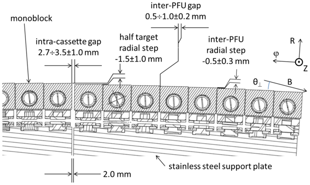
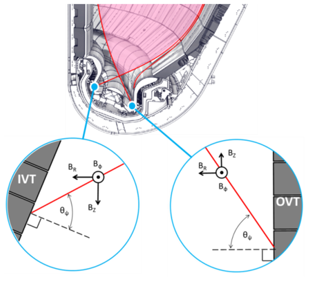
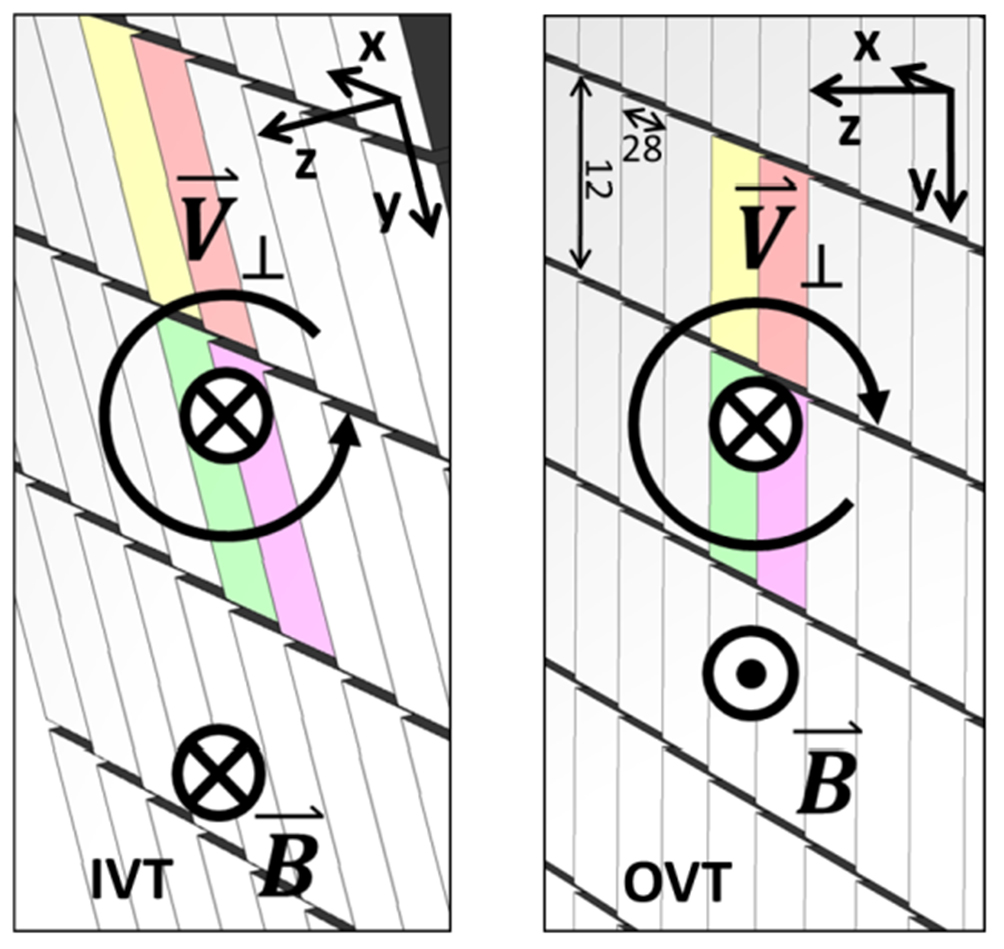
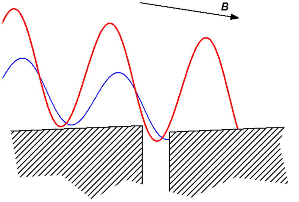
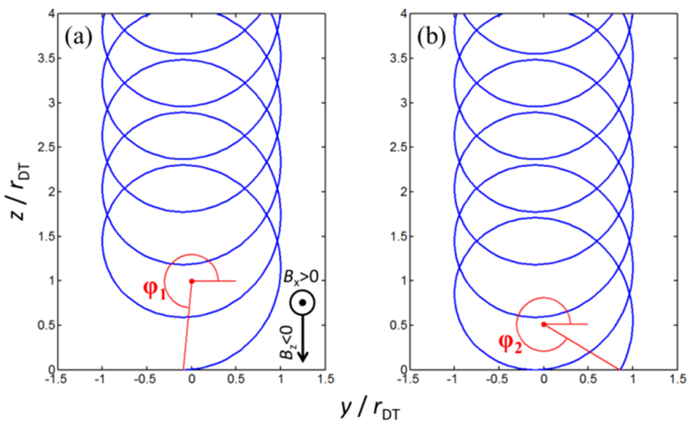
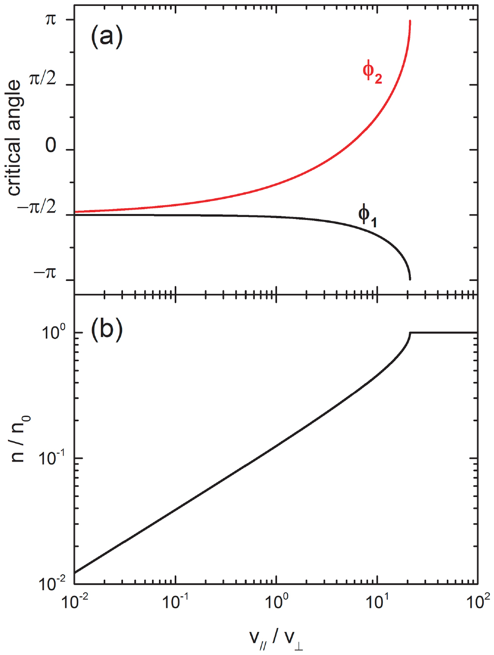
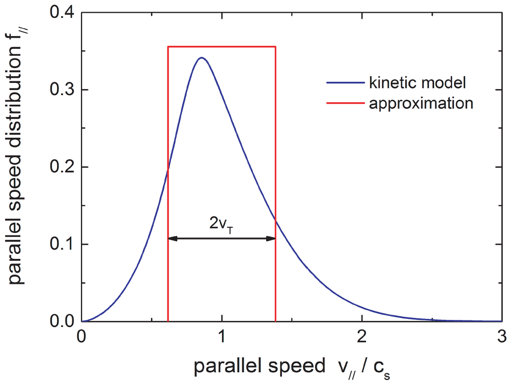
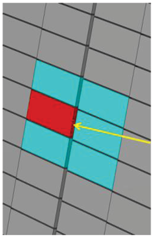
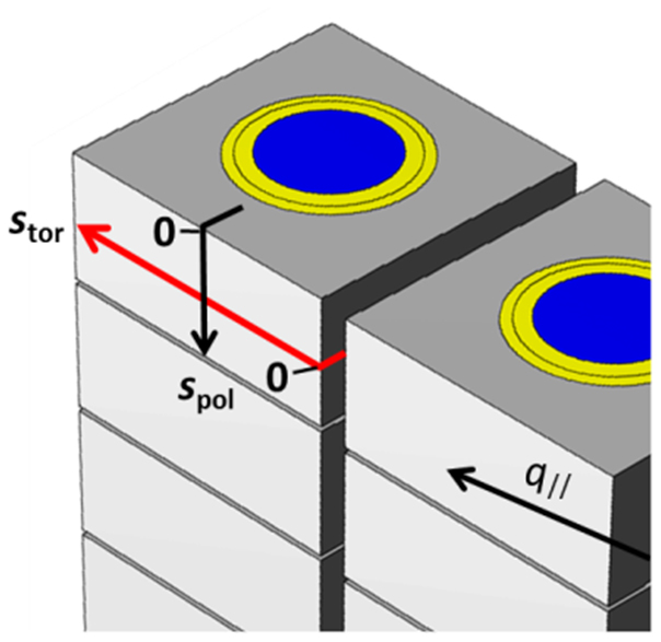
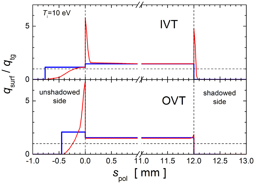
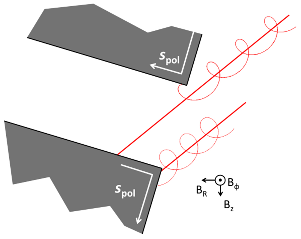
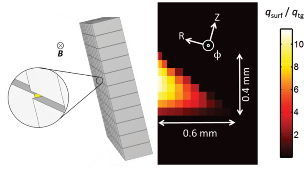
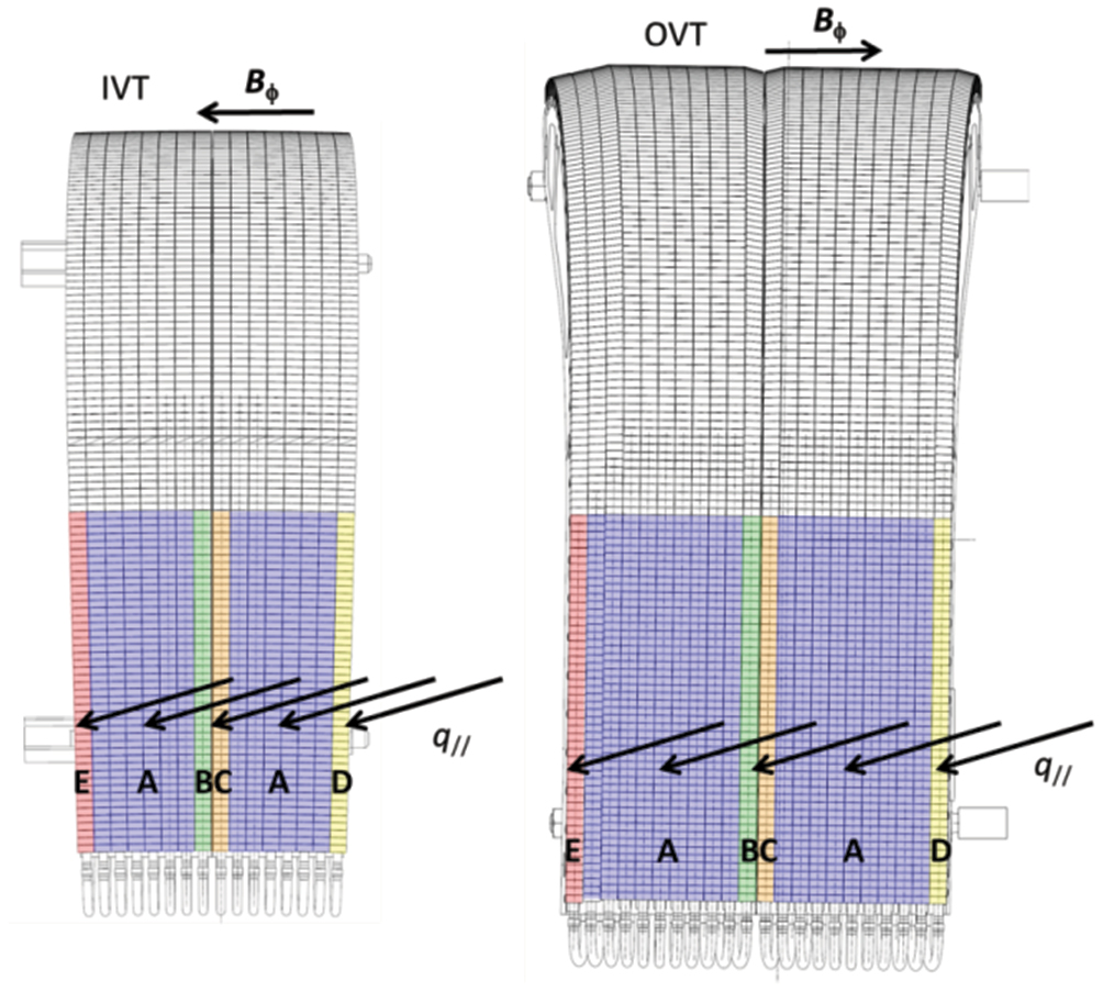
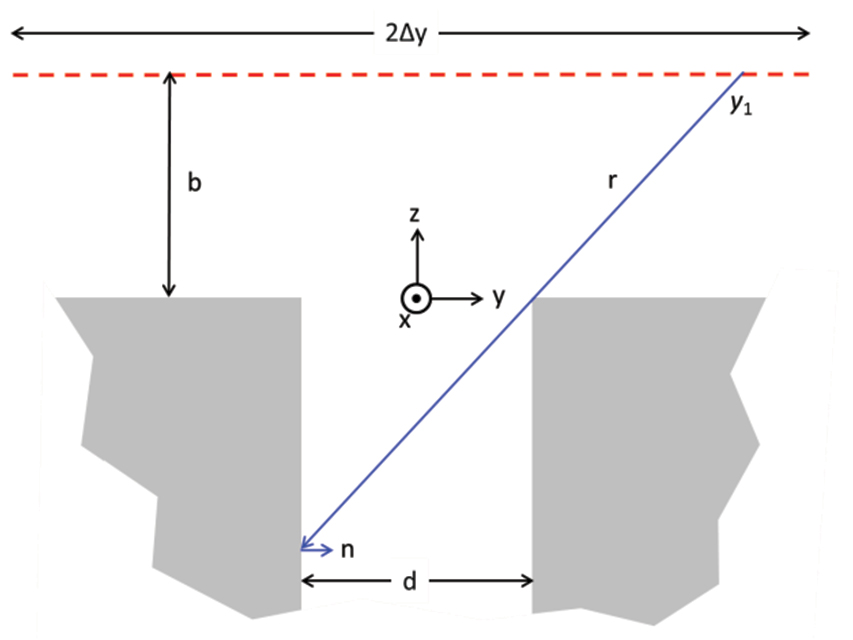
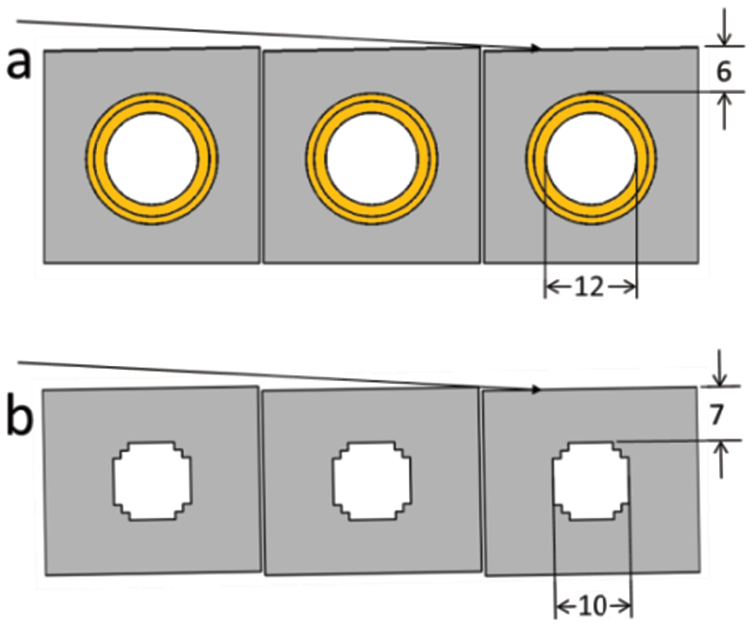
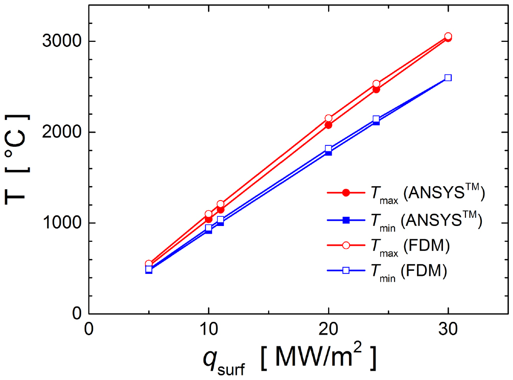
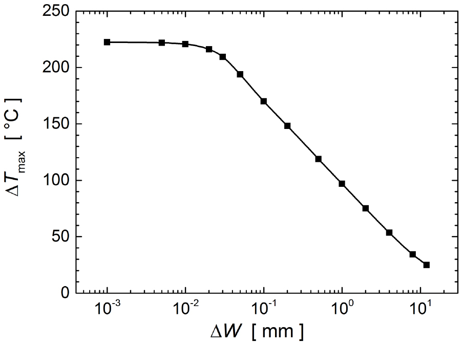
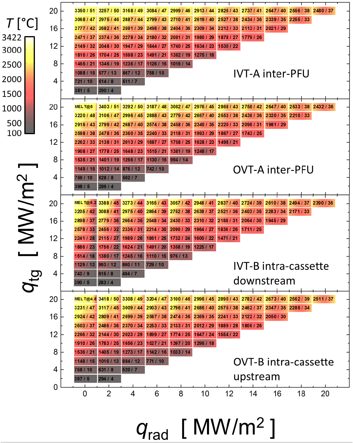
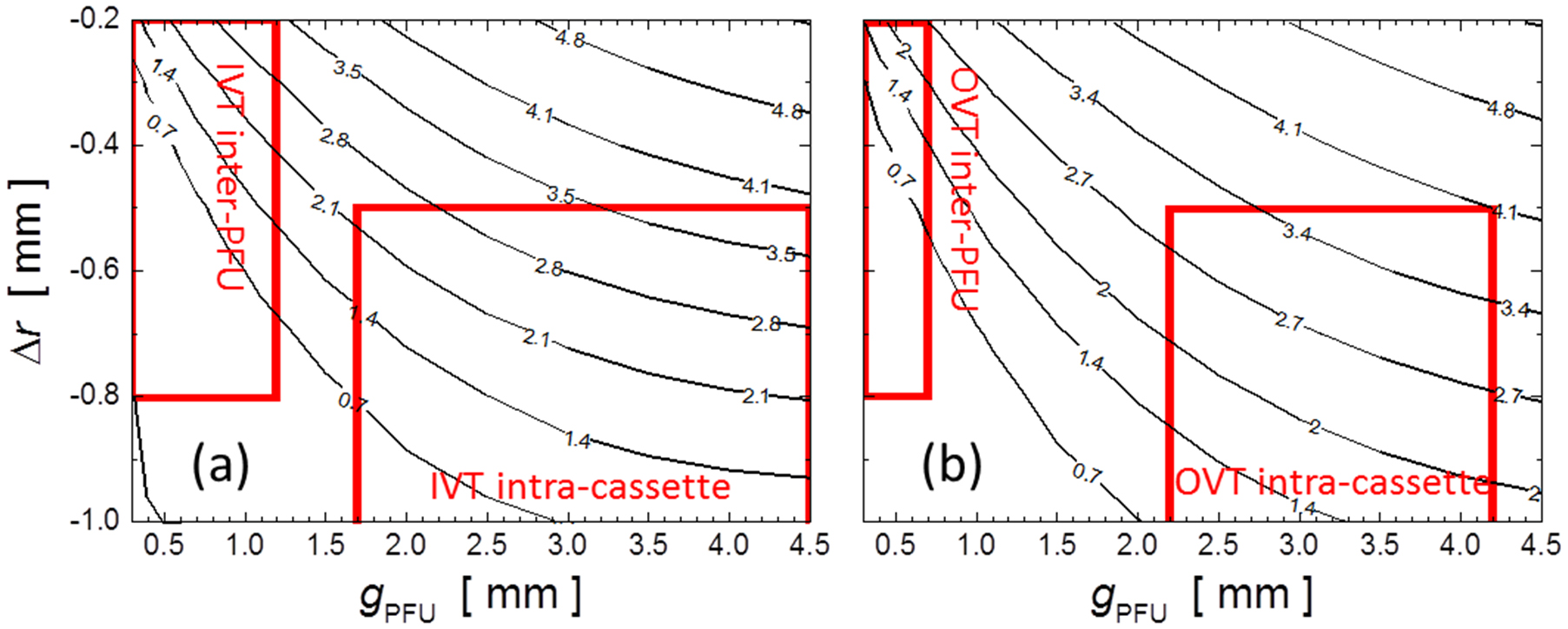
Figure 49. The shaded area indicates the range of expected ELM energy fluences in ITER based on a recent empirical scaling law [4] (which does not contain information about an isotope dependence since the experiments were all performed in deuterium plasmas). The left axis scale corresponds to the parallel energy fluence released during ELM events, while the right axis scale indicates its projection onto the nominal ITER OVT. Full and open stars: the minimum energy fluence that raises the surface temperature to the melting threshold at the monoblock top surfaces and the upper toroidal edges, respectively. Full circles: energy fluence that gives a factor two margin against full surface melting. The dashed lines indicate the operating points of 5 MA and 7.5 MA pre-nuclear scenarios in H and D/He, respectively, and the 15 MA DT nuclear burn.
Download figure:
Standard image High-resolution image
Table 5. Evaluation of risk of melting W monoblocks by uncontrolled ELMs in three ITER operation scenarios.
| Scenario | Full surface melting? | Edge melting? |
|---|---|---|
| Pre-nuclear hydrogen 5MA | Avoided with wide margin | Avoided with narrow margin (less than 2) |
| Pre-nuclear D or He 7.5 MA | Avoided with narrow margin (less than 2) | Possible during largest ELMs |
| DT nuclear burn 15 MA | Unavoidable | Unavoidable |
7. Conclusions
The proposed design of the ITER divertor vertical targets consists of actively cooled tungsten monoblocks whose top surfaces are beveled to a depth of htor = 0.5 mm in the toroidal direction in order to magnetically shadow poloidal leading edges arising from assembly and manufacturing tolerances. This shaping solution appears to be mandatory to avoid bulk melting in stationary operation [15]. Neither burring nor poloidal profiling to protect toroidal edges is foreseen, mainly to avoid the increased cost and manufacturing complexity that more sophisticated shaping solutions imply. Moreover, scoping studies of alternative shaping solutions such as edge chamfering, edge filleting, and poloidal beveling have been carried out and shown to offer no viable solutions to the toroidal edge heating problem [49] at the IVT (an equivalent study at the OVT has also been performed but the results are still being evaluated at the time of writing of this paper).
A systematic study of the detailed 3D heat flux distribution on the top surfaces and inside the gaps between monoblocks and the resulting thermal response due to steady inter-ELM heat loads and transient ELM loads for a range of ITER operating scenarios has been performed using ion orbit modelling. Comparison with self-consistent PIC simulations has shown that the results obtained with this model, which takes account of Larmor gyration but ignores sheath electric fields, are qualitatively, and in many cases, quantitatively correct [8]. PIC calculations of this problem require formidable computing power and long run times which may exceed several months. The simple model described here executes in a few minutes on a personal computer and thus provides a powerful tool to perform scoping studies for a large number of cases in a relatively short time.
Shaping strategies to hide exposed leading edges work, but at the expense of reduced power-handling capacity of the monoblocks. Target tilting and monoblock toroidal bevel increase the angles of magnetic field line (and hence thermal plasma) incidence, which are near glancing to begin with (~3°), so the additional 1.5° added by shaping increases the local plasma component of the heat flux by ~50% in inter-ELM periods and during ELMs. In the worst case of negligible radiated power, the monoblock temperature increase, which varies nearly linearly with heat flux, is therefore 50% higher than the temperatures obtained in high heat flux tests, with the following consequences for inter-ELM periods:
- (1)The highest temperature occurs at the unshadowed trailing edges where the path of the heat flux streamlines to the cooling channel is the longest. This temperature is set by the local heat flux; it depends only slightly on toroidal wetted fraction. The peak monoblock temperature is thus practically independent of inter-PFU misalignments.
- (2)At the peak stationary heat fluxes of qtg ~ 10 MW m−2 which ITER sets as its maximum operating point during the burning plasma, steady state phase, the surface temperature can marginally rise to the upper end of the recrystallization range of 1000–1300 °C or even exceed it when the radiated power is negligible compared to the plasma component. For the SOLPS baseline case with pure neon seeding, for example, the radiated power produces only qrad ~ 1 MW m−2 for a total qtg = 10 MW m−2 (and therefore qsurf ~ 9(1.5) + 1 = 14.5 MW m−2 real power density), and the resulting temperature exceeds 1400 °C over the entire surface, with values up to 1800 °C at the trailing edge. For higher radiated fractions that would be expected with nitrogen seeding, the surface temperatures would be lower at the center of the monoblock above the cooling tube (~1200 °C for qrad ~ 4 MW m−2), but still high at the trailing edge. It can be noted that certain W grades have recently demonstrated evidence of higher recrystallization temperatures [33] approaching ~1700 °C.
- (3)During slow transient reattachment events, where the peak power density may attain up to qtg ~ 20 MW m−2 for several seconds, the monoblock trailing edge will be very close to, if not slightly above melting. We note that the thermal properties of recrystallized tungsten are degraded, so melting could occur even earlier, depending on the operational history of any given MB. Even if marginal melting could be accepted, there is a risk of burn-out because the margin against critical heat flux is lost. To recover that margin, as well as the temperatures attained in high heat flux electron beam tests at 20 MW m−2, the slow transient heat load specification would have to be decreased to qtg ~ 15 MW m−2.
The ion orbit model does not predict any new phenomena of profound consequences for monoblock heat handling during stationary inter-ELM power handling phases, or in cases in which the divertor heat flux density increases on a slow timescale (plasma reattachment events). The ion Larmor radius is so small that the optical approximation remains valid in most cases (the only exception is at the lower monoblock edges on the IVT where ions can spiral onto the magnetically shadowed surface). A recent coordinated international campaign of experiments has re-confirmed the validity of the optical approximation for plasmas characteristic of inter-ELM periods [15]. In general, there is some additional heating, which can attain a few 100 °C, of monoblock edges and of the optical hot spot that appears on leading edges adjacent to gap crossings. Radiative heating of the sides of monoblocks facing into wide inter- and intra-cassette gaps can increase the temperature by a similar amount. These increments are important in a system that is already critical without taking them into account. For example, power focusing onto toroidal edges produces a local temperature increase that can attain ~200 °C during slow transient reattachment. This supplements the high temperature at the trailing edge and is responsible for pushing the surface over the melting temperature. The additional inter-ELM heating due to optical hot spots, on the other hand, is of no concern, since the power falls on a region that is mostly shadowed and thus cooler.
The high monoblock temperatures and concomitant loss of critical heat flux margin are a result of the increased local heat flux brought about by monoblock bevel and component tilting. There is no shaping solution which can change that. The implementation of shaping to avoid poloidal leading edge melting thus imposes a reduction on the allowed poloidal heat flux to the divertor targets. This in turn will feed back on the operational window and thus potentially on achievable fusion performance, although this is a very complex, multi-parameter issue which is likely only to be fully resolved once ITER exploitation begins.
Concerning ELMs, the ion orbit model reveals a number of new, critical phenomena that require further study. The penetration of hot ions into magnetically shadowed poloidal gaps is facilitated by their large Larmor radii. A single uncontrolled ELM in the 15 MA burning plasma phase is predicted to melt the poloidal leading edges of most monoblocks at the strike zone, except those that are the most deeply recessed within the specified assembly tolerances. The most critical result concerns the long toroidal edges and monoblock corners. Larmor radius focusing is predicted to melt the lower (upper) toroidal monoblock edges at the inner (outer) vertical targets even during pre-nuclear operation at half toroidal field and plasma current. Melting at these locations could be problematic, since unlike the poloidal edges, the toroidal ones receive the full inter-ELM heat loads. Edge melting would likely be avoided in 5 MA/1.8 T hydrogen plasmas. On the other hand, monoblock corners at the poloidal leading edges of both vertical targets will melt in any plasma scenario with uncontrolled ELMs.
If it is found that edge and corner melting is not detrimental to ITER operation, then only the avoidance of full surface melting remains as an issue. The margin against melting is reduced by the additional tilt of the monoblock surfaces which increases their power loading by ~50%, but even more by the fact that monoblocks will be already hot due to the steady inter-ELM loads. In pre-nuclear plasma scenarios, full surface melting during uncontrolled ELMs should be avoided with a sufficient margin, if the recent scaling for outer target parallel ELM energy fluences [4] applies at the ITER scale. In the full performance burning plasma scenario, full surface melting by uncontrolled ELMs will be unavoidable, making the successful implementation of effective mitigation techniques indispensable.
That full surface melting by uncontrolled ELMs will be unavoidable in the burning plasma phase has been anticipated since the beginning of research in this field. This analysis identifies the new issues of edge melting, and a greatly reduced margin against full surface melting. According to these calculations, the limit to avoid full surface melting is one order of magnitude smaller than the historical limit of εtg = 0.5 MJ m−2 in the burning nuclear phase. The principal reason for this limit is the high temperature of the monoblocks, which is very close to half the melting temperature of tungsten and makes achieving a factor two margin nearly impossible. In fact, given the proximity to half the melting temperature along with the accumulation of various uncertainties, pragmatism would lead us to conclude that 100% ELM suppression is required. Full surface melting begins for energy fluence of about εtg = 0.6 MJ m−2 which is likely to occur, according to the empirical scaling law [4], if ELMs are not mitigated.
The simple analysis performed in this scoping study is by no means the last word on this topic. A number of issues have been raised that now require serious investigation in existing tokamaks and high heat flux facilities. Continued extension of the multi-machine scaling of ELM energy flux densities is essential, especially at the inner divertor target, as are improvements to ELM modelling. The calculations developed here apply to nominal, as-manufactured monoblocks. The first melt event that occurs will change the surface relief, so more sophisticated calculations involving melt layer motion, combined with ion orbit calculations, are needed to anticipate the evolution of the damaged zones and the risks for tokamak performance. The results compiled here can serve as a basis for identifying research issues that should be urgently addressed in anticipation of ITER operation. Most particularly, the prediction of Larmor radius focusing of heat flux onto poloidal and toroidal edges requires experimental confirmation. In existing machines it should be possible to design an experiment to obtain ELM ions with Larmor radii that are larger than the width of a specially constructed gap. Even if the appropriate dimensionless parameter regime can certainly be achieved, ELM energies in most tokamaks are typically no more than a few tens of kJ, so detecting fine-scale leading edge flash heating by means of infra-red thermography could be a challenge.
Acknowledgments
This work was supported within the framework of a contract between the CEA and ITER, the SSA 29—ITER/IA/13/ 4300000827 'Full-W divertor: assessment of target monoblock shaping for the safe operation of the ITER machine'.
Disclaimer
The views and opinions expressed herein do not necessarily reflect those of the ITER Organization. ITER is the nuclear facility INB 174.
Footnotes
- 8
Throughout this paper the 'top' surface of the MBs is a shorthand expression that refers to the plasma-facing surface, in reference to the local Cartesian coordinate system, defined below, in which the z-axis coincides with the surface normal vector. When referring to the long toroidal edges of the MBs, they are distinguished by the words 'upper' and 'lower' in the sense that an observer standing in the divertor would employ them to describe what she or he sees, with respect to the Earth's gravity.
- 9
The energy fluence is the total energy deposited per unit surface area, given by the time integral of the surface heat flux during an ELM event, and has units of J m−2. This quantity has been incorrectly called 'energy flux' [52], which has units of W m−2, or 'energy density' [50], which has units of J m−3. Here we adopt the correct term which is employed in the field of radiology [42].