
Contemporary Trends in High and Low River Flows in Upper Indus Basin, Pakistan
by
 , and
, and
Muhammad Yaseen
1, 
Yasir Latif
2,3,*,
Muhammad Waseem
4,
Megersa Kebede Leta
5,*,
Sohail Abbas
6 and
and
Haris Akram Bhatti
7 1
Centre for Integrated Mountain Research (CIMR), Qaid e Azam Campus, University of the Punjab, Lahore 53720, Pakistan
2
Institute of Computer Sciences, Czech Academy of Sciences, 18207 Prague, Czech Republic
3
Key Laboratory of Tibetan Environment Changes and Land Surface Processes, Institute of Tibetan Plateau Research, Chinese Academy of Sciences, Beijing 100101, China
4
Department of Civil Engineering, Ghulam Ishaq Khan Institute of Engineering Sciences and Technology, Topi 23460, Pakistan
5
Faculty of Agriculture and Environmental Sciences, University of Rostock, 18059 Rostock, Germany
6
Climate Research Institute, Konkuk University, Seoul 100011, Korea
7
Department of Civil Engineering, NED University of Engineering and Technology, Karachi 75200, Pakistan
*
Authors to whom correspondence should be addressed.
Water 2022, 14(3), 337; https://doi.org/10.3390/w14030337
Submission received: 12 November 2021
/
Revised: 1 January 2022
/
Accepted: 3 January 2022
/
Published: 24 January 2022
(This article belongs to the Section Hydrology)
Abstract
:The Upper Indus Basin (UIB) features the high mountain ranges of the Hindukush, Karakoram and Himalaya (HKH). The snow and glacier meltwater contribution feeds 10 major river basins downstream including Astore, Gilgit, Hunza, Jhelum, Kabul, Shyok and Shigar. Climate change is likely to fluctuate the runoff generated from such river basins concerning high and low streamflows. Widening the lens of focus, the present study examines the magnitude and timing of high flows variability as well as trends variability in low streamflows using Sen’s slope and the Mann-Kendall test in UIB from 1981 to 2016. The results revealed that the trend in the magnitude of the high flows decreased at most of the sub-basins including the Jhelum, Indus and Kabul River basins. Significantly increased high flows were observed in the glacier regime of UIB at Shigar and Shyok while decreased flows were predominant in Hunza River at Daniyor Bridge. A similar proclivity of predominantly reduced flows was observed in nival and rainfall regimes in terms of significant negative trends in the Jhelum, Kunhar, Neelum and Poonch River basins. The timing of the high flows has not changed radically as magnitude at all gauging stations. For the low flows, decreasing significant trends were detected in the annual flows as well as in other extremes of low flows (1-day, 7-day, 15-day). The more profound and decreasing pattern of low flows was observed in summer at most of the gauging stations; however, such stations exhibited increased low flows in autumn, winter and spring. The decrease in low flows indicates the extension of dry periods particularly in summer. The high-water demand in summer will be compromised due to consistently reducing summer flows; the lower the water availability, the lower will be the crop yield and electricity generation.
1. Introduction
Climate change appears to accelerate the hydrological cycle which is expected to increase the frequency and impact of extreme events such as droughts and floods [1,2,3,4]. The hydrological cycle may impact significantly the water resources due to changing climate [5,6]. The changes in temperature intensity and precipitation pattern have a direct influence on the quantity of evapo-transpiration and runoff [7,8]. Consequently, the spatial and temporal water resource availability will be negatively affected, which will have serious repercussions on major sectors such as agriculture, industry and urban development [9,10,11].
The Upper Indus Basin (UIB) is constituted by high elevated glaciers in the Hindukush-Karakoram-Himalaya (HKH), covering an area of 32,182 km2 [12]. Over the past decade, the changing climate and concerning hydro-meteorological implications on glaciers in the HKH attracted efforts from the scientific community towards the assessment of the glacier dynamics in terms of glacier retreat, advancement, stability, or the surge-like stability [13,14,15,16]. Many studies have assessed changes in precipitation, temperature and stream flow [17,18,19,20,21,22,23,24,25,26,27,28]. The main Indus is predominantly fed by glacial melt generated by Karakoram glaciers which are also affected by precipitation and temperature changes [17,29]. The UIB is a region where the assessment of annual and seasonal distribution of river flows is prone to compromise due to changing climate and catastrophic impacts on snow, precipitation and glaciers.
Furthermore, most of the rivers are unregulated, with more than 50 years of continuous flow data showing a great climatic variability in trends occurring [30]. The winter temperature drops to freezing levels, and the same temperature increases in summer, feeding rivers with rainfall, snow, and glaciers in major sub basins of the UIB. The timing of river flow is dictated by the relative amount of precipitation occurring as rain (immediate) runoff or snow (delayed) directly affects the seasonal flow variation [26,31,32]. Increased/decreased precipitation alter the flow timings in ablation season depending upon the timing and quantity of precipitation. [33,34,35].
Streamflow regimes refer to the variation of flow over space and time, and the related time scales vary from minutes to decades [36,37]. Flow regimes calculation is associated with the climate change risks regarding freshwater availability [38]. Climate change impacts humans and freshwater ecosystems in terms of flow seasonality; inter-annual variability; and statistically low, mean and high flows, floods and droughts. Variations in flow regime affect humans with respect to water storage/supply, meandering, electricity production and flooding events [38].
The trends in the annual maximum, medium and low streamflow in rivers were found significant [39]. Flood trend studies tend to focus on trends in the annual maximum flood series. The unusual stage of a river is called flood; therefore, the annual flows are important in terms of flood control, storage and mitigation infrastructure. The river water quality and aquatic ecosystems are directly affected by the values of these indicators which represent severity of hydrological droughts occurred annually/seasonally and have been generally used for designing safe water abstractions and waste load allocations.
Severe floods of various magnitudes occurred in Pakistan during 1950, 1956, 1957, 1973, 1976, 1978, 1988, 1992, 2010 and in 2013. Punjab, Sindh, Khyber Pakhtunkhwa (KPK), Baluchistan, FATA, Gilgit-Baltistan, Azad Jammu Kashmir (AJK) and some areas of the Punjab were severely affected by these floods. The financial losses amounted to more than USD 30 billion during the past 60 years. Particularly, during the period from 1950 to 2009, there was a financial loss of USD 20 billion together with 8887 deaths, 109,822 villages damaged/destroyed and an overall area of 407,132 km2 was compromised [40]. In view of recent dramatic floods, detection of trends in long time series of flood data is of scientific interest and practical importance. The assumption of a stationary hydrological process, i.e., river stage or discharge, is necessary for planning of future water resources and flood protection. Major floods in Pakistan during the past decade have raised the question of whether or not they are an effect of a changing climate.
In Pakistan changes in flow magnitudes (high/low) create major issues on water divide on provincial level particularly in the downstream areas (Sindh province). It includes less water availability during the dry season and high flooding in the ablation period. The impact of a changing climate may alter the operational role of existing water resources in terms of capacity and planning for new installation [41,42]. However, most studies [17,18,19,26,43,44] conducted in UIB were restricted to mean flow, and no study has addressed the variability in maximum and minimum flows. Specifically, [17] presented an analysis of eight stations in the period 1966–2005, and [26] analyzed 19 stations in the period 1961–1998. Most of the earlier studies were restricted to annual flows with a smaller number of gauging stations [21,22,27,28]. Some studies covered the whole UIB including Kabul and Jhelum River basins [27,28]; however, they used only annual or seasonal flows for trend detection.
Previously, several significant papers have been published in the same study area using more or less similar gauging stations with different data periods and study objectives [44,45,46,47,48]. Some of them used innovative methods for flow measurements in UIB [44] while others analyzed trends variability in hydroclimatic variables [36]. Several focused-on snow cover variability, flows simulation and restricted to hydrological modelling rather than trend analysis [46,47,48]. Most importantly, a few studies addressed the hydrology of UIB comprehensively mentioning the mass balance, flow regime, contribution and limitations of station data available for such sort of analyses [36]. The objective of this investigation is to identify the variability and trend analysis in magnitude and timing of high as well as low river flows of mountainous catchments in UIB including the Jhelum and Kabul River basins. The temporal resolution covers the maximum available data based on daily records from 1981 to 2016 for all gauging stations in three major river basins. To accomplish the desired goal, the peak flow date and the maximum/minimum value of daily mean flow were calculated during that year.
2. Study Area and Dataset
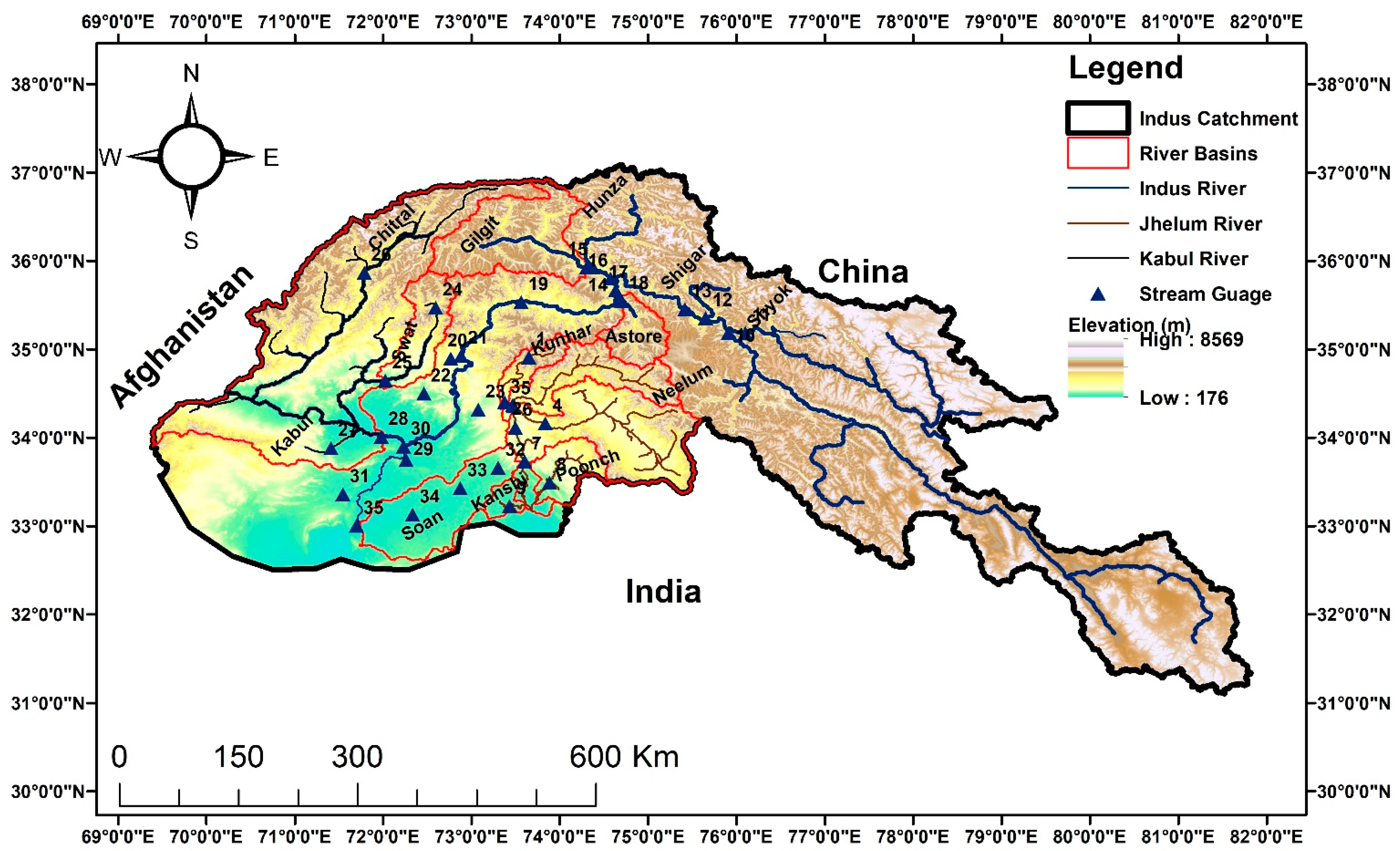
The UIB represents a transboundary basin which shares borders with Afghanistan, China (Tibet), India and Pakistan, and its high mountain HKH ranges present a hydrological zone [45]. For the Hunza River Basin, the relevant hydrological region lies above 5000 m, where maximum snowfall occurs [48]. They further explained that the snow cover extends to around 80% and squeezes around up to 30% in the summer. The hydrology of the UIB was addressed defining its three major regimes in which flow was generated by different sources of moisture input as shown in Figure 1. The selection of the gauging station was carried out keeping in view the sources of moisture. For instance, high flows are restricted to 22 gauging stations while the low flow analysis was extended to 35 gauging stations. The selected region also contains the Astore, Gilgit and Hunza sub-basins of the UIB which feature different geographical aspects, and streamflow is generated due to the westerlies, but it acts differently to these basins [36]. The generated runoff in the ablation season is not restricted to glaciers in high altitude but gets fed by perennial and seasonal snow/ice, snow covered areas and monsoon precipitation [45]. These authors further explained that a high elevation range (4500–6500) is quite unique where it snows even in the peak ablation period (July–September). The Jhelum River originates in Pir Panjal and flows along the Indus at an elevation of 5500 feet. It is one of the most important rivers among the eastern tributaries which feed the Indus River system.
In Pakistan, the second largest dam was built on the Jhelum River, which serves partly to generate electricity and also for water storage purposes, throughout the year. Pakistan holds 45% of the total area of the Kashmir valley which is commonly known as Azad Kashmir, and the rest of the area is occupied by India. Mangla reservoir is fed by five sub-catchments including Jhelum, Poonch, Kanshi, Neelum/Kishan Ganga and Kunhar. The Neelum is the highest contributor to the flow, being the largest tributary of the Jhelum, which contributes at Domel followed by the Kunhar River of the Kaghan valley which meets the Jhelum at Kohala Bridge.
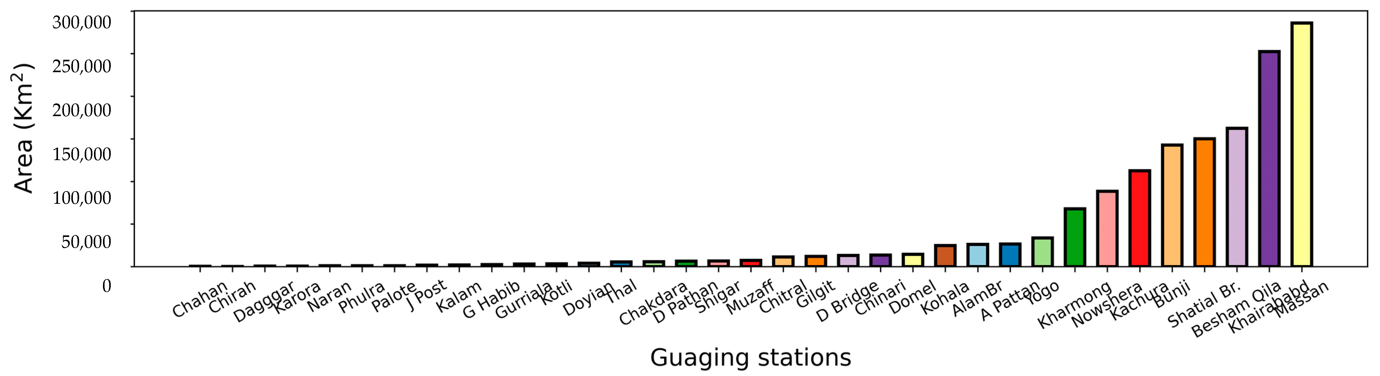
The Water and Power Development Authority—Surface Water Hydrology Project (WAPDA-SWHP) has established the network of streamflow measurement in UIB beginning in 1960 [28]. The number of installed gauges in all sub-basins is 35 as shown in Figure 1. The high flow data was restricted to of 22 gauging stations; however, the low flows were observed at all 35 gauges for the period 1981–2016. Three major basins, Jhelum, Indus and Kabul, constitute the study area with 22 sub-basins. There are some gauges which cover a large area (Massan, Khairabad and Bunji) while three of them represent a small drainage area of less than 500 km2 (Chirah and Chahan) as shown in Figure 2. The selection of the non-uniform number of gauges is attributed to the geographical importance of gauges. Those gauges were excluded for high flows where no record threat of flooding was observed due to the very low range of high flows. However, for the analysis of low flows, all 35 gauges were used. Moreover, some of the gauges for high flows did not have the same data range; therefore, analysis was restricted to 1981–2016. Annual high and low flows for each year are based on daily data. Means of magnitude and timing of annual high flows together with 1 to 15 days low flows for the Period of 1981–2016 are given in Table 1. Two indices were used to describe the characteristics of the upper end of the flow regime, i.e., the floods. The first index addresses the magnitude in terms of the annual maximum daily mean river flow (annual maximum) while, the second deals with the timing of annual high flows. Similarly, their extremes were observed in low flows concerning 1-day, 7-day and 15-day.
3. Materials and Methods
Parametric or non-parametric statistical tests confirm the existence of significant statistical trends [33]. Non-parametric tests in trend analysis are recommended in hydro climatological time series due to their robustness, while also ignoring missing values. The magnitude and peak flow timings were assessed using the non-parametric Mann-Kendall test [11,34] due to the nonlinear nature of river flows. The test was firstly used by Mann while test distribution was carried out by Kendall [49]. For further use, the test does not need any other sort of confirmation for data distribution which makes it and extraordinary tool for the detection. However, the existence of serial correlation creates noise in time series data which must be removed by pre-whitening to eliminate the serial correlation. It is generally known as the trend free pre-whitening technique (TFPW) used by recent studies [27,28]. The slope of flows was estimated by Sen’s method [50]. All three tests are recommended for trend detection in hydro climatological time series [33,51,52,53,54,55].
3.1. Trend Detection
Some studies [55] proposed the uniformity in MK and Spearman tests. Keeping this fact in view, the application of the MK and SS methods enabled trend and slope detection, respectively, in the time series of flow indices. A challenging problem with the MK test is that the result contains noise due to the serial correlation structure of the time series. Therefore, various approaches have been suggested in the literature to address the effect of autocorrelation on the outcome of the test.
3.2. Serial Correlation Effect
Within a data series, existence of an auto/serial correlation directs the MK test to indicate a false trend significance [56]. To overcome this issue, [57] proposed the use of pre-whitening. Some studies [51] successfully eliminated the serial correlation and its association with the MW test. Some studies [58] modified the pre-whitening method, the TFPW, to treat the noise in time series due to serial correlation. This modified test has been widely used in the recent studies for noise free trend detection in hydro meteorological time series [21,26,27,28].
Change in per unit time (slope) (β) is calculated by the Sen’s approach followed by detrending of the time serious assuming the absence of nonlinear trend. The next step involves the assessment of the lag-1 serial correlation (r1). MK is directly applied to the original values if the r1 appears as insignificant at the 5% level. Conversely, TFPW is carried out.
3.3. Mann–Kendal Test for Trend Detection
The non-parametric test is free from normal distribution of data and does not require or is less sensitive towards the homogenization of the time series data which makes it a perfect trend detector [59].
The Mann-Kendall statistic zmk was evaluated as follows:
The MK statistic S is calculated as
where n shows the number of years; xj and xk are values (annual) in years j and k, correspondingly. The function sgn (xj − xk) decides that either the value 1, 0 or −1 should be employed depending upon the difference of (xj − xk), where j > k:
zmk shows an increasing trend with a positive value and vice versa. If the probability with null hypothesis Ho exceeds the test statistic zmk for selected significance level α, it indicates the presence of a significant trend where the test statistic (S) must follow the standard normal distribution. In the null hypothesis, Ho stands correct in the absence of any trends using the standard normal table to reject Ho. For the assessment of To being either a positive or negative trend at α level of significance, Ho is rejected if the absolute value of zmk > z1−a/2 at the α-level of significance.
3.4. Sen’s Slope
Sen’s formula enabled the variation within the selected data series using the slope value. Such variation over time was estimated relative to mean daily discharge. The relative units were used, as discharge varies significantly between the two gauges, and therefore, absolute change comparison is daunting. The inter comparison becomes difficult due to the small magnitude of change in daily discharge.
N pairs of data were computed in the first phase using the following relation:
The Sen’s estimator of slope shows the median of these N values of Q. The median of the N slope is calculated in the common way. N values of Qi were arranged from minimum to maximum.
The Sen’s estimator given as follow:
Ultimately, Qmed uses a double-tailed test with 100(1 − α)% confidence interval while Sen’s method enabled true slope.
4. Results
4.1. Variability and Trend Detection in Magnitude of High Flows
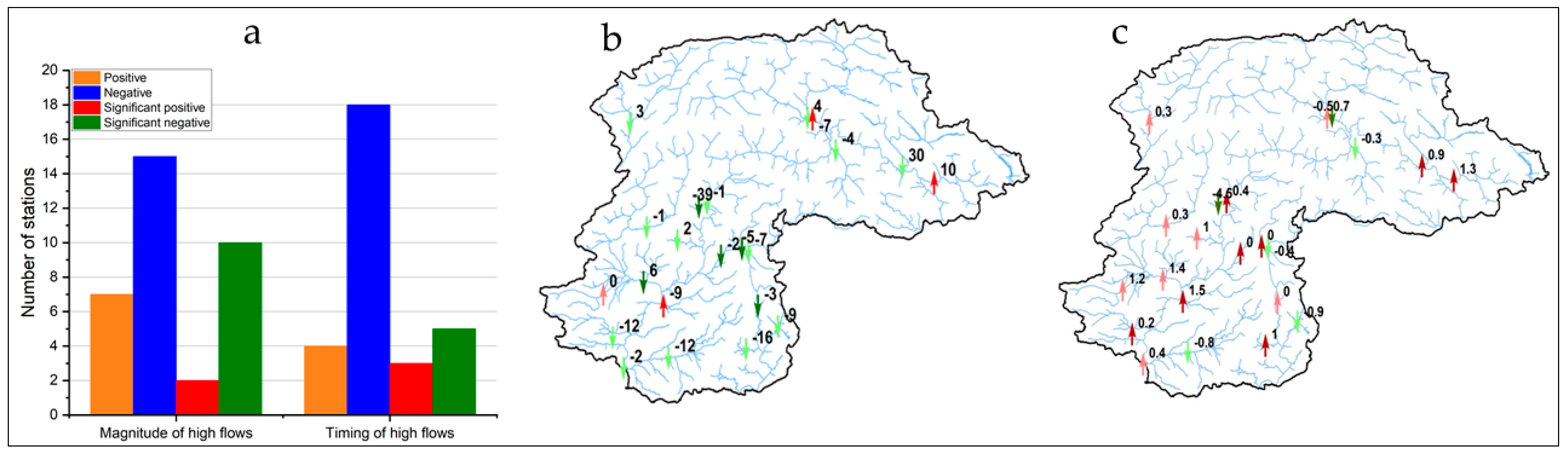
Annual maximum flows exhibited negative trends at 15 (10 significant) stations while positive trends were shown by 7 (2 significant) between 1981 and 2016 as shown in Figure 3a. The Jhelum River basin at Mangla dam and its tributaries (Kunhar, Neelum, Poonch and Kanshi Rivers) revealed decreasing trends. These trends were found significant at the Jhelum, Kunhar, Neelum and Poonch River basins while insignificant at the Neelum and Kanshi River basins as shown in Figure 3b.
For the Kabul River Basin, annual maximum flows increased at Nowshera at a rate of 6%, but the trends were statistically insignificant. The Chitral and Bara tributaries of the Kabul River Basin exhibited increasing trends while flows decreased at Swat. The Hunza river flows exhibited negative a significant trend with 7% decrease in mean maximum flow (1494 cumec). The Hunza river is fed predominantly by glacier melt followed by snow and precipitation. The Shyok, Shigar and Gilgit river basins showed significantly increasing trends except Gilgit with rates of 10%, 30% and 4%, respectively. The Haro (significant with p < 0.01), Kurram (significant with p < 0.01) and Soan (insignificant) tributaries of the Indus have a decreasing trend with rates of 9%, 12% and 12%, respectively. The Indus River at Besham Qila/Tarbella showed significantly (p < 0.05) negative trend at a rate of 1%.
4.2. Variability and Trend Detection in Timing of High Flows
The northern rivers of UIB are more sensitive towards the temporal changes rather than the spatial changes. The peak flow appears between June and August as shown in Table 1. Particularly, the peaks in glacier dominant basins appear in August as compared to the snow dominant basin where it occurs in the beginning of June [28,46,47]. Most changes in peak timing with significant trends occurred from late 1981 to 2016. The decreases in the timing of annual high flows were found in 18 (5 significant) stations while the timing increased in 4 (3 significant) stations for the period 1981–2016 as shown in Figure 3a. Only four rivers/sub-basins (Shyok, Hunza, Bara and Haro) of UIB exhibited an increasing trend in flows. The frequencies of annual high flows in the Jhelum River basin at Mangle dam and its tributaries (Kunhar, Neelum, Poonch and Kanshi Rivers) increased, however, significant trends were restricted to Kunhar and Jhelum rivers as shown in Figure 3c.
The Indus at Tarbela dam and Kabul Rivers also showed significantly (p < 0.05) negative trends with rates of of 0.2 and 0.3 days/decade, respectively. The highest negative trend (significant with p < 0.01) was found Siran River with a rate of 2.2 days/decade. The Rivers Swat and Kunhar at Chitral have a subsiding trend, whereas Bara River showed a cumulative tendency. The change in dates over time probably is related to the amount and timing of spring snowmelt. Giglit, Astore and Jhelum River basins are considered as snow predominant basins where the snowmelt contribution remains higher than the glacier and rainfall. These basins exhibited significant trends in early ablation period in terms of winter/spring flow. The plots of annual time series of timing of high flows in different rivers of UIB are shown in Figure 4. The timing of high flow is different depending upon the melting source and basin hydrology. The high peaks appeared in early July at Kabul and Kunhar rivers. However, such high peaks shifted to late July at Gilgit, Indus at Terbela and Soan Rivers. For the Jhelum basin, the high peak appeared in the early ablation season, i.e, June 18 at Mangla Dam. This peak appears earlier at high altitude sub-basins of the Jhelum River. The highest flow was observed on 02 August in the Hunza River Basin at Danyior Bridge. This peak might be attributed to perennial snow and glacier contribution as seasonal snow disappears (melting) in July.
4.3. Variability and Trend Detection in Magnitude of Low Flows
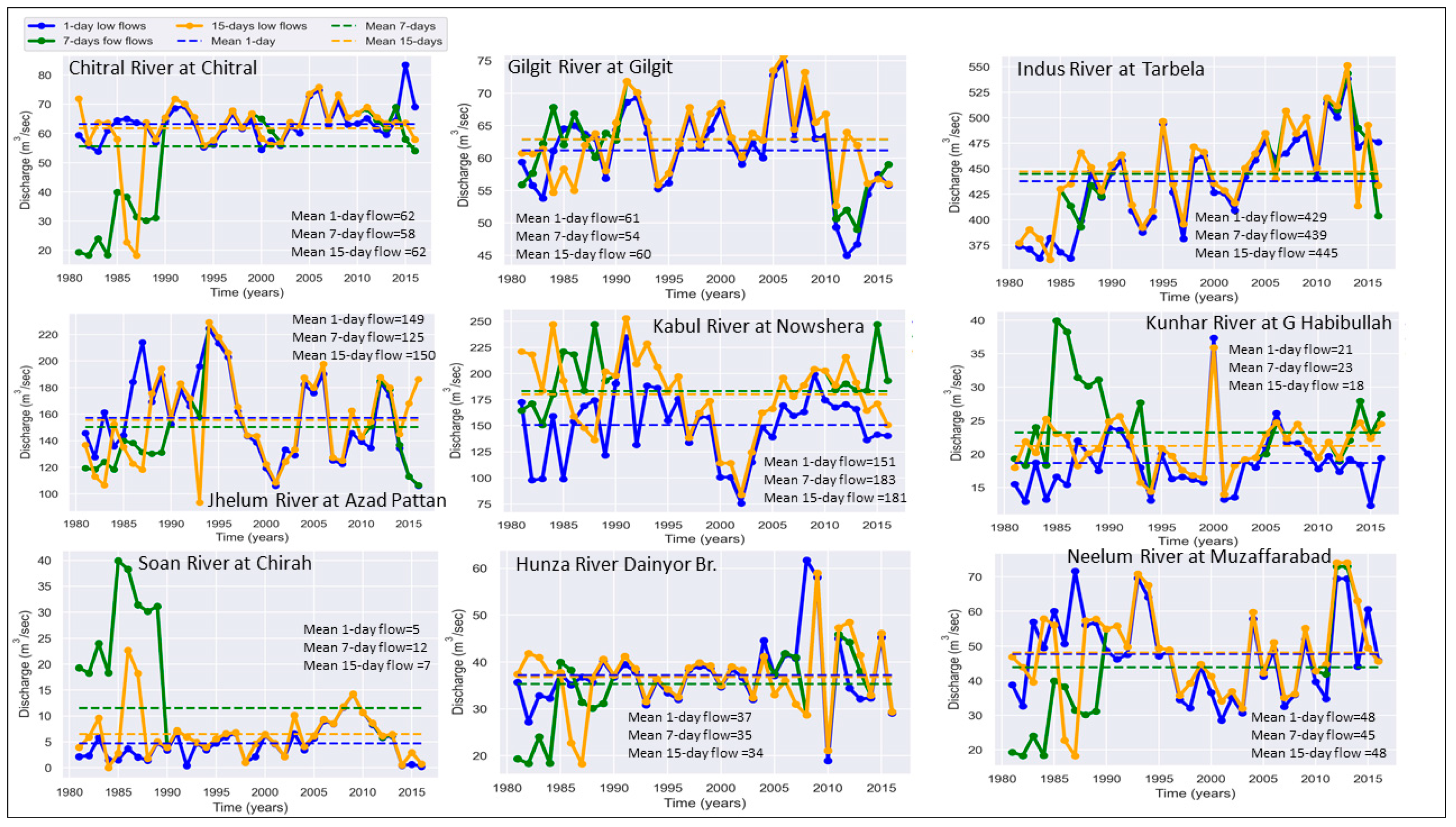
Trends in low flows at different time scale, i.e., 1-day, 7-day and 15-day in annual and seasonal time series for 35 stations were investigated for the period of 1981–2016. These trends were detected by applying the same MK test at the significance level of 90%, 95%, 99% and 99.99%. The trend value (change vale) in these time series was estimated through the Sen’s slope method. After filtering the present data, 35 different stations were marked, upon which analysis was performed. The time series analysis of major rivers having low flows is given in Figure 5. The highest low and lowest low flows were exhibited at the Indus and Soan Rivers, respectively. The mean low flow at Daniyor Bridge in the Hunza River falls to 34 m3/s in 15 consecutive days, remaining with 1400 m3/s as mean maximum in the ablation season. Similarly, the low flow at Indus at Tarbella could have a 15-day low flow means of 445 m3/s, reaching a highest flow mean in summer of 10,700 m3/s. Generally, a slightly increasing trend was observed in low flows at most of the gauges for all three extremes. Spatial maps were developed, and the geographical location of different stream gauges with increasing or decreasing trends are shown in various figures.
4.3.1. Trends in 1-Day Low Flows
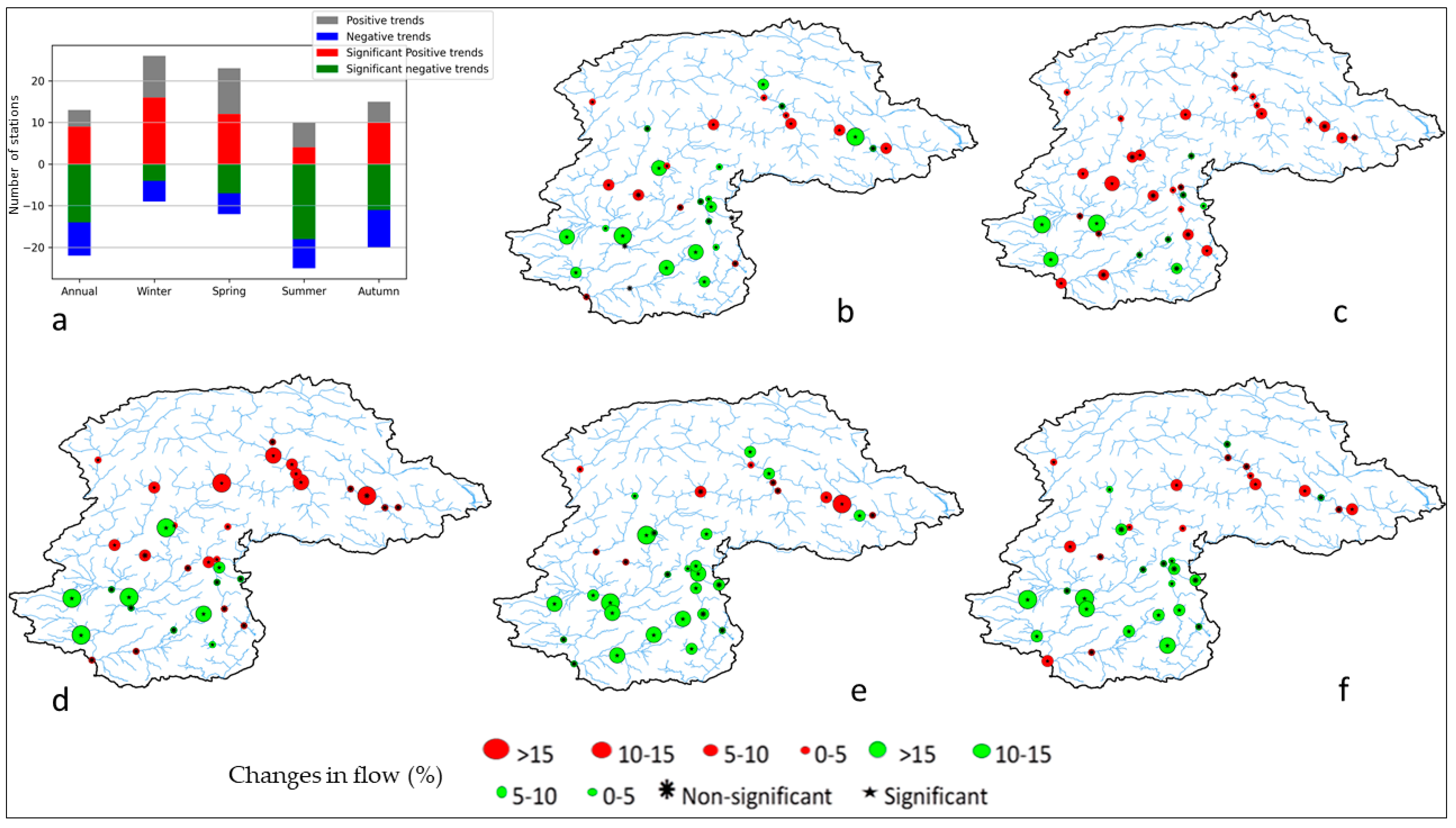
The results of the MK test for annual and seasonal 1-day low flows at 35 hydrological stations of UIB for the time series of 1981–2016 are shown in Figure 6. Annual 1-day low flows have significantly decreased at 14 stations and increased at 9 stations as shown in Figure 6a. The proclivity of decreasing trends indicates the overall reduced water availability in UIB. The highest decreasing trend was observed with 34% in the Indus Basin (at Khairabad), 14% in the Kabul Basin (at Jhansi Post) and 10% in the Jhelum Basin (at Palote). Similarly, the seasonal analysis proposed decreased summer and autumn flows while increased winter and spring flows. The overall high decreasing trend was observed at Khairabad (Indus River) but increased by 6% at Massan (Indus) with a 95% significance level. The 1-day flow decreased significantly with rates of 57%, 40%, 29% and 42% for winter, spring, summer and autumn, respectively, in the Indus basin (at Khairabad).
4.3.2. Trends in 7-Day Low Flows
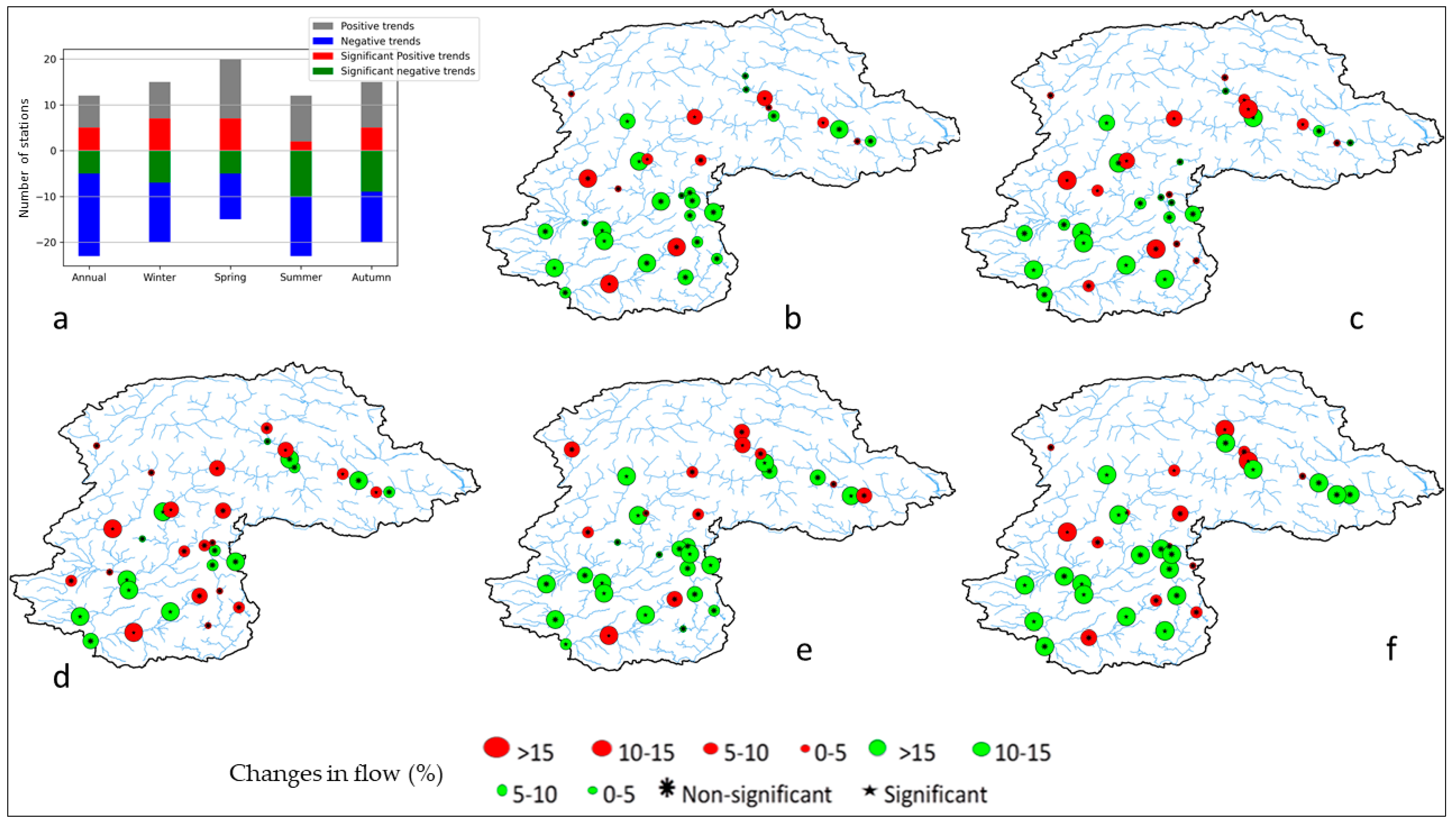
The annual and seasonal streamflow trends for 7-day low flows were analyzed and detected as shown in Figure 7. There was a close call between the number of stations (05) exhibiting significant negative trends and the stations (05) showing positive trends in annual time series as shown in Figure 7a. Similarly, in seasonal variation, the maximum number of negative trends were observed in summer followed by autumn, spring and winter. However, the maximum number of stations exhibiting positive flows were observed in spring followed by autumn, winter and summer. The trends in summer were significant at Karora (Indus River) with 36% decreasing (99.9% significance), at Jhansi Post (Kabul Basin) with 12% (95% significance), Muzaffarabad (Neelum River) 8% (95%) at Khairabad (Indus River) showed 55% (95% significance).
The seasonal changes significantly appeared in winter and summer in terms of predominantly decreasing trends in summer rather than winter. Significantly decreasing trends appeared at 10 stations while increasing at only at 2 in summer. However, autumn low flows increased at 5 stations while decreasing at 9 stations as shown in Figure 7a. In winter, the numbers of increasing/decreasing trends were almost equal; however, increased spring flows were observed at 7 stations as compared to decreased trends at 5 stations. In winter the highest decreasing trend was observed at Khairabad and Jhansi Post with rates of 54% (99.9%significant) and 10% (99% significance), respectively. In spring it was observed at Khairabad, Karora, Jhansi Post and Thal, 59% (99.9%significant), 27% (99.9% significance), 5% (99% significance) and 40% (99% significance), respectively. In summer, it was observed at Khairabad and Karora, 19% (99% significance), 41% (99.99 significant) and in autumn at Khairabad and Jhansi Post, 56% (99.9% significance), 14% (99% significance), correspondingly. The greatest frequency of a significantly negative trend was observed at Khairabad (Indus River) 55% (99.9% significance) annually, 54% in winter, 59% in spring, 19% in summer, and 56% in autumn.
4.3.3. Trends in 15-Day Low Flows
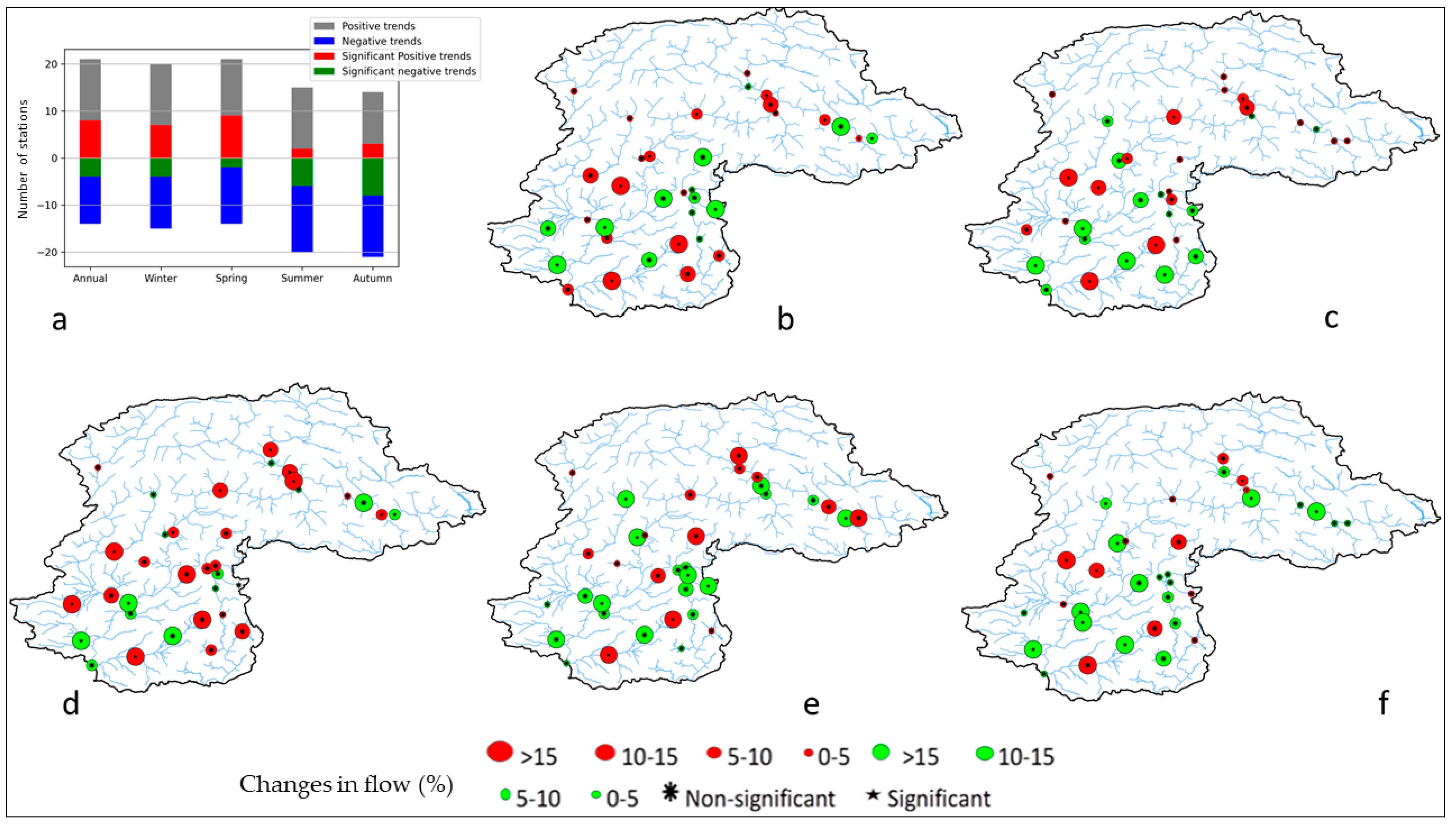
The temporal and spatial distribution of annual and seasonal variations in 15-days flow is shown in Figure 8. The number of stations (08) exhibiting significant negative trends was higher as compared to the stations (4) showing positive trends as shown in Figure 8a. Similarly, the maximum number of negative trends were appeared in autumn followed by summer, winter and spring. However, the maximum number of stations exhibiting positive flows were observed in spring followed by winter summer and autumn. The highest decreasing trend in annual time series was observed at Khairabad, Shigar, Jhansi Post and Naran 48% (99.9% significance), 19% (99% significance), 11% (95% significance), 16% (99.9% significance), respectively, as shown in Figure 8b.
In winter season, the highest decreasing trends were detected at Khairabad and Kotli 48% (99.9% significance), 10% (99% significance), in spring Khairabad, Jhansi Post, Thal and Karora 52% (99.9% significance), 20% (99% significance), 32% (99% significance), 19% (99.9% significance). In summer Khairabad and Karora 17 (99% significance), 5% (99.9% significance), while in autumn, Khairabad and Jhansi Post 52% (99.9% significance) and 3% (99% significance) were detected showing maximum decreasing trends in streamflow. Astonishingly, the magnitude of negative trends is much higher as compared to the positive trends, which means flows are reducing at higher rate due to seasonal shifts, amount of precipitation and melting behavior at high altitudes.
5. Discussion
The present study observed the predominance of decreasing trends based on annual and seasonal time series analysis of low and high flows in UIB. The gauging stations were installed within a diverse range, from high glaciated mountains to the lower reaches of downstream areas. A similar variation of high and low flows was observed at spatial and temporal scale annually and seasonally within all the selected sub-basins. Based on the previous results, UIB presents a conflicting signal of climate [18] in terms of cooler summer and contrasting hydrological regime (decreasing flows) [21]. Similar trends were observed by a previous study covering some of the stations in Indus and Jhelum [19]. These results can be divided according to the temporal scale of annual, seasonal, monthly and daily and the spatial scale of large to small river basins based on the hydrology, moisture input and melting behavior of the concerned basin observed by various studies. According to the previous observations, the Muzaffarabad gauging station (Jhelum Basin) exhibited positive trends from May to August while negative trends in June and July [21]. Similar negative summer trends were observed by recent studies [28]. The predominant behavior of summer negative trends was observed by [28] for the whole summer (June-August) and particularly in June. These authors included the month of September in summer to observe the late ablation period in which the glacier regime contributes maximum flow as compared to snow-fed basins due to the early melting of snow in peak ablation. The annual and summer low flows significantly decreased, which is consistent with the earlier studies. The flow gauging stations selected in the Karakoram range were Shigar at Shigar, Shyok at Yogo and Daniyor Bridge at Hunza. The high flows observed at these stations are completely consistent with [60,61] who proposed increased flows at Shigar and Shyok while decreased flows at Daniyor Bridge (Hunza River). Similarly, the increasing trends of flows align with the recent studies [28,62,63].
The predominant decreasing trends of the Hunza basin have been previously discussed by [21] who linked the falling trends with negative summer temperature trends [28] and negative mass balance [29]. The increasing trend in the snow-fed basins is linked to the amount of winter precipitation and melting in summer [6,21,28,64]. The outcomes of this study are consistent with [27,28,29,60,63] which might be attributed to land use land cover changes (LULC) as observed in other parts of the world [65,66].
The obtained results not only broaden our knowledge about the hydrology of the UIB but also have considerable applicative potential. The detection of trends and variability of the Indus River with the use of the copula function can help to formulate adaptation strategies and reconsider existing regional development plans, including management projects for irrigation schemes, flood protection, hydropower generation and sustainable water resources planning in that area and in these regions of Pakistan, which benefit from the UIB’s water.
It can be said that the negative trend in mean flows affects the dimensions, and hence, the construction cost of the dam can be also considered as a limiting factor for the water quantity withdrawn from the reservoir and storage capacity due to changing climate concerning variability in hydroclimatic trends [67,68,69]. Therefore, it may be concluded that low flows are decreasing annually and seasonally in summer and autumn. The decrease in low flows is important for the location of the water treatment facility, quantity of irrigation and drinking water. The changes in low-flow statistics also affect the minimum water quantity released by dams downstream for the sustainable protection of ecological cycles. The decrease in annual mean flows, on the other hand, plays a predominant role in the determination of water reservoir capacity and in the reservoir, management works afterwards.
6. Conclusions
This study analyzed the contemporary trends in the magnitude and timing of high and low streamflows at different hydrological stations installed in major sub-basins of the UIB for the period 1981–2016. TFPW enabled the elimination of serial correlation from the low and high flow time series data before detecting trends. The MK and Sen’s methods were applied to observe the significance and slope of the observed trends, respectively. According to the findings, the magnitude and timings of annual maximum/high flows have decreased at most of the sub-basins included the main Jhelum, Indus and Kabul Rivers. Most changes in peak timing having significant trends occurred from late 1981 to 2016. The Shyok, Shigar and Gilgit river basins exhibited positive significant trends at the rates of 10%, 30% and 4%, respectively. The Indus at Tarbela dam and Kabul Rivers have also a significant decreasing trend (p < 0.05) at the rates of 0.2 and 0.3 day/decade, respectively. Results revealed that the overall decreasing significant trends were prevalent in annual mean flow as well as in other statistics of low flows (1 Day, 7 Day, 15 Day low flows). It was also observed that summer and autumn low flows decreased while winter and spring low flows increased. Counter to common belief, the most profound and decreasing pattern of flows was observed in summer; however, winter exhibited increased flows progressively extending to spring. The decrease in low flows indicates the extension of dry periods particularly in summer. The high-water demand in summer will be compromised due to the reducing summer flows; the lower the water availability, the lower will be the crop yield and the electricity generation.
The present study was limited to flow analyses only covering the temporal range up to 2016; however, the interpretation of results was carried out keeping in mind the recent trends of temperature, precipitation and snow cover variation in Indus, Indus, Jhelum and Kabul River basins of UIB. The temporal range can be extended further, and the impact of variation of high and low flows can be linked to temperature, precipitation and snow cover on a sub-basin scale using a degree-day or energy-based model. However, the spatial gap of some gauges is vast, due to which the precise flow variability in high as well as low flows can be significantly compromised.
Author Contributions
Conceptualization, M.Y., Y.L.; methodology, M.Y., Y.L., S.A., M.W. and S.A.; software, M.Y., Y.L.; validation, M.K.L. and M.W.; formal analysis, M.Y., Y.L., S.A. and H.A.B.; investigation, M.Y., Y.L., M.W., M.K.L. and S.A.; writing—original draft, M.Y.; writing—review and editing, M.Y. and Y.L.; visualization, M.K.L., Y.L. and H.A.B.; supervision, M.K.L.; funding acquisition, M.K.L. and M.W. All authors have read and agreed to the published version of the manuscript.
Funding
This research received no external funding.
Institutional Review Board Statement
Not applicable.
Informed Consent Statement
Not applicable.
Conflicts of Interest
The authors declare no conflict of interest.
References
- Durodola, O.S. The Impact of Climate Change Induced Extreme Events on Agriculture and Food Security: A Review on Nigeria. Agric. Sci. 2019, 10, 487–498. [Google Scholar] [CrossRef] [Green Version]
- Raikes, J.; Smith, T.F.; Jacobson, C.; Baldwin, C. Pre-disaster planning and preparedness for floods and droughts: A systematic review. Int. J. Disaster Risk Reduct. 2019, 38, 101–207. [Google Scholar] [CrossRef]
- Snyder, K.A.; Evers, L.; Chambers, J.C.; Dunham, J.; Bradford, J.B.; Loik, M.E. Effects of changing climate on the hydrological cycle in cold desert ecosystems of the Great Basin and Columbia Plateau. Rangel. Ecol. Manag. 2019, 72, 1–12. [Google Scholar] [CrossRef]
- Sy, S.; Quesada, B. Anthropogenic land cover change impact on climate extremes during the 21st century. Environ. Res. Lett. 2020, 15, 034002. [Google Scholar] [CrossRef]
- Bates, B.C.; Kundzewicz, Z.W.; Wu, S.; Palutikof, J. Climate Change and Water. In Technical Paper of the Intergovernmental Panel on Climate Change; IPCC Secretariat: Geneva, Switzerland, 2008. [Google Scholar]
- Archer, D.R.; Fowler, H.J. Spatial and temporal variations in precipitation in the Upper Indus Basin, global teleconnections and hydrological implications. Hydrol. Earth Syst. Sci. 2004, 8, 47–61. [Google Scholar] [CrossRef] [Green Version]
- Akbar, R.; Short Gianotti, D.J.; Salvucci, G.D.; Entekhabi, D. Mapped hydroclimatology of evapotranspiration and drainage runoff using SMAP brightness temperature observations and precipitation information. Water Res. Res. 2019, 55, 3391–3413. [Google Scholar] [CrossRef]
- Abbas, S.; Mayo, Z.A. Impact of temperature and rainfall on rice production in Punjab, Pakistan. Environ. Dev. Sustain. 2020, 23, 1–23. [Google Scholar] [CrossRef]
- Uprety, M.; Ochoa-Tocachi, B.F.; Paul, J.D.; Regmi, S.; Buytaert, W. Improving water resources management using participatory monitoring in a remote mountainous region of Nepal. J. Hydrol. Reg. Stud. 2019, 23, 100604. [Google Scholar] [CrossRef]
- Wang, Y.; Wang, Y.; Su, X.; Qi, L.; Liu, M. Evaluation of the comprehensive carrying capacity of interprovincial water resources in China and the spatial effect. J. Hydrol. 2019, 575, 794–809. [Google Scholar] [CrossRef]
- Khan, N.; Shahid, S.; Bin Ismail, T.; Wang, X.J. Spatial distribution of unidirectional trends in temperature and temperature extremes in Pakistan. Theor. Appl. Climatol. 2019, 136, 899–913. [Google Scholar] [CrossRef]
- Eriksson, M.; Jianchu, X.U.; Shrestha, A.B.; Vaidya, R.A.; Nepal, S.; Sandstörm, K. The Changing Himalayas: Impact of Climate Change on Water Resources and Livelihoods in the Greater Himalayas; ICIMOD: Kathmandu, Nepal, 2009. [Google Scholar]
- Hewitt, K. Geomorphic hazards in mountain environments. In Mountain Geomorphology; Owens, P.N., Slaymaker, O., Eds.; Arnold: London, UK, 2004; pp. 187–218. [Google Scholar]
- Bookhagen, B.; Burbank, D.W. Toward a complete Himalayan hydrological budget: Spatiotemporal distribution of snowmelt and rainfall and their impact on river discharge. J. Geophys. Res. 2010, 115, F03019. [Google Scholar] [CrossRef] [Green Version]
- Thøgersen, K.; Gilbert, A.; Schuler, T.V.; Malthe-Sørenssen, A. Rate-and-state friction explains glacier surge propagation. Nat. Commun. 2019, 10, 2823. [Google Scholar] [CrossRef] [PubMed]
- Kääb, A.; Berthier, E.; Nuth, C.; Gardelle, J.; Arnaud, Y. Contrasting patterns of early twenty-first-century glacier mass change in the Himalayas. Nature 2012, 488, 495–498. [Google Scholar] [CrossRef]
- Hewitt, K. The karakoram anomaly, glacier expansion and the elevation effect Karakorum Himalaya. Mt. Res. Dev. 2005, 25, 332–340. [Google Scholar] [CrossRef] [Green Version]
- Fowler, H.J.; Archer, D.R. Conflicting Signals of Climate Change in the Upper Indus Basin. J. Clim. 2006, 19, 4276–4292. [Google Scholar] [CrossRef] [Green Version]
- Fowler, H.J.; Archer, D.R. Hydro-climatological variability in the Upper Indus Basin and implications for water resources. In Regional Hydrological Impacts of Climatic Change—Impact Assessment and Decision Making; Wagener, T., Franks, S.W., Eds.; IAHS Publication: Oxfordshire, UK, 2005; Volume 295, pp. 131–138. [Google Scholar]
- Archer, D. Contrasting hydrological regimes in the upper Indus Basin. J. Hydrol. 2003, 274, 198–210. [Google Scholar] [CrossRef]
- Sharif, M.; Archer, D.; Fowler, H.; Forsythe, N. Trends in timing and magnitude of flow in the Upper Indus Basin. Hydrol. Earth Syst. Sci. 2013, 17, 1503–1516. [Google Scholar] [CrossRef] [Green Version]
- Ahmadalipour, A.; Moradkhani, H.; Demirel, M.C. A comparative assessment of projected meteorological and hydrological droughts: Elucidating the role of temperature. J. Hydrol. 2017, 553, 785–797. [Google Scholar] [CrossRef] [Green Version]
- Ahmadalipour, A.; Moradkhani, H. A data-driven analysis of flash flood hazard, fatalities, and damages over the CONUS during 1996–2017. J. Hydrol. 2019, 578, 106–124. [Google Scholar] [CrossRef]
- Latif, Y.; Ma, Y.; Ma, W.; Muhammad, S.; Muhammad, Y. Snowmelt runoff simulation during early 21st century using hydrological modelling in the snow-fed terrain of Gilgit river basin (Pakistan). Advances in sustainable and environmental hydrology, hydrogeology, hydrochemistry and water resources (chapter 18). In Proceedings of the 1st Springer Conference of the Arabian Journal of Geosciences (CAJG-1), Hammamet, Tunisia, 12–15 November 2018. [Google Scholar]
- Do, H.X.; Zhao, F.; Westra, S.; Leonard, M.; Gudmundsson, L.; Boulange, J.E.S.; Müller Schmied, H. Historical and future changes in global flood magnitude–evidence from a model-observation investigation. Hydrol. Earth Syst. Sci. 2020, 24, 1543–1564. [Google Scholar] [CrossRef] [Green Version]
- Forsythe, N.; Archer, D.R.; Pritchard, D.; Fowler, H. A Hydrological Perspective on Interpretation of Available Climate Projections for the Upper Indus Basin. In Indus River Basin; Elsevier: Amsterdam, The Netherlands, 2019; pp. 159–179. [Google Scholar]
- Yaseen, M.; Ahmad, I.; Guo, J.; Azam, M.I.; Latif, Y. Spatiotemporal Variability in the Hydrometeorological Time-Series over Upper Indus River Basin of Pakistan. Adv. Meteorol. 2020, 2020, 1–18. [Google Scholar] [CrossRef]
- Latif, Y.; Ma, Y.; Ma, W. Climatic trends variability and concerning flow regime of Upper Indus Basin Jehlum, and Kabul River Basins. Theor. Appl. Climatol. 2021, 144, 447–468. [Google Scholar] [CrossRef]
- Farinotti, D.; Immerzeel, W.W.; de Kok, R.J.; Quincey, D.J.; Dehecq, A. Manifestations and mechanisms of the Karakoram glacier Anomaly. Nat. Geosci. 2020, 13, 8–16. [Google Scholar] [CrossRef] [PubMed]
- Anderson, J.J. Decadal Climate Cycles and Declining Columbia River Salmon. In Sustainable Fisheries Management: Pacific Salmon; CRC Press LLC: New York, NY, USA, 2020; pp. 467–484. [Google Scholar]
- Frederick, S.E.; Woodhouse, C.A. A multi century Perspective on the Relative Influence of Seasonal Precipitation on Streamflow in the Missouri River Headwaters. Water Resour. Res. 2020, 56, e2019WR025756. [Google Scholar] [CrossRef]
- Bilal, H.; Chamhuri, S.; Mokhtar, M.B.; Kanniah, K.D. Recent snow cover variation in the Upper Indus Basin of Gilgit Baltistan, Hindukush Karakoram Himalaya. J. Mt. Sci. 2019, 16, 296–308. [Google Scholar] [CrossRef]
- Abbas, S.; Kousar, S.; Yaseen, M.; Mayo, Z.A.; Zainab, M.; Mahmood, M.J.; Raza, H. Impact assessment of socioeconomic factors on dimensions of environmental degradation in Pakistan. SN Appl. Sci. 2020, 2, 468. [Google Scholar] [CrossRef] [Green Version]
- Abbas, S.; Shirazi, S.A.; Qureshi, S. SWOT analysis for socio-ecological landscape variation as a precursor to the management of the mountainous Kanshi watershed, Salt Range of Pakistan. Int. J. Sustain. Dev. World Ecol. 2018, 25, 351–361. [Google Scholar] [CrossRef]
- Anwar, A.A.; Bhatti, M.T. Pakistan’s water apportionment Accord of 1991: 25 years and beyond. J. Water Resour. Plan. Manag. 2018, 144, 05017015. [Google Scholar] [CrossRef] [Green Version]
- Archer, D.R.; Forsythe, N.; Fowler, H.J.; Shah, S.M. Sustainability of water resources management in the Indus Basin under changing climatic and socio-economic conditions. Hydrol. Earth Syst. Sci. 2010, 14, 1669–1680. [Google Scholar] [CrossRef] [Green Version]
- Asfaw, A.; Simane, B.; Hassen, A.; Bantider, A. Variability and time series trend analysis of rainfall and temperature in northcentral Ethiopia: A case study in Woleka sub-basin. Weather Clim. Extrem. 2018, 19, 29–41. [Google Scholar] [CrossRef]
- Höök, T.O.; Foley, C.J.; Collingsworth, P.; Dorworth, L.; Fisher, B.; Hoverman, J.T.; LaRue, E.; Pyron, M.; Tank, J. An assessment of the potential impacts of climate change on freshwater habitats and biota of Indiana, USA. Clim. Change 2019, 163, 1–20. [Google Scholar] [CrossRef]
- Carling, P.A.; Huang, H.Q.; Su, T.; Hornby, D. Flow structure in large bedrock-channels: The example of macroturbulent rapids, lower Mekong River, Southeast Asia. Earth Surf. Process. Landf. 2019, 44, 843–860. [Google Scholar] [CrossRef]
- FFC (2010) Ministry of Water and Power of Pakistan. Annual Flood Report 2010, Islamabad, Pakistan, WAPDA.Shakir, A.S.; Rehman, H.; Ehsan, S. Climate Change Impact on River Flows in Chitral Watershed. Pak. J. Eng. Appl. Sci. 2010, 7, 12–22. [Google Scholar]
- Tigkas, D.; Vangelis, H.; Tsakiris, G. Implementing Crop Evapotranspiration in RDI for Farm-Level Drought Evaluation and Adaptation under Climate Change Conditions. Water Resour. Manag. 2020, 34, 1–15. [Google Scholar] [CrossRef]
- Garee, K.; Chen, X.; Bao, A.; Wang, Y.; Meng, F. Hydrological modeling of the upper Indus basin: A case study from a high-altitude glacierized catchment Hunza. Water 2017, 9, 17. [Google Scholar] [CrossRef] [Green Version]
- Tarar, Z.R.; Ahmad, S.R.; Ahmad, I.; Majid, Z. Detection of sediment trends using wavelet transforms in the upper Indus River. Water 2018, 10, 918. [Google Scholar] [CrossRef] [Green Version]
- Sobkowiak, L.; Perz, A.; Wrzesiński, D.; Faiz, M.A. Estimation of the River Flow Synchronicity in the Upper Indus River Basin Using Copula Functions. Sustainability 2020, 12, 5122. [Google Scholar] [CrossRef]
- Mukhopadhyay, B.; Khan, A. A quantitative assessment of the genetic sources of the hydrologic flow regimes in Upper Indus Basin and its significance in a changing climate. J. Hydrol. 2014, 509, 549–572. [Google Scholar] [CrossRef]
- Akhtar, M.; Ahmad, N.; Booij, M.J. The impact of climate change on the water resources of Hindukush—Karakorum—Himalaya region under different glacier coverage scenarios. J. Hydrol. 2008, 355, 148–163. [Google Scholar] [CrossRef]
- Bhutiyani, M.R.; Vishwas, S.K.; Pawar, N.J. Changing streamflow patterns in the rivers of northwestern Himalaya: Implications of global warming in the 20th century. Curr. Sci. 2008, 95, 618–626. [Google Scholar]
- Tahir, A.A.; Chevallier, P.; Arnaud, Y.; Ahmad, B. Snow cover dynamics and hydrological regime of the Hunza River basin, Karakoram Range, Northern Pakistan. Hydrol. Earth Syst. Sci. 2011, 15, 2821–2860. [Google Scholar] [CrossRef] [Green Version]
- Kendall, M.G. Rank Correlation Methods, 4th ed.; Charles Griffin: London, UK, 1975. [Google Scholar]
- Sen, P.K. Estimates of regression coefficients based on Kendall’s tau. J. Am. Stat. Assoc. 1968, 63, 1379–1389. [Google Scholar] [CrossRef]
- Yue, S.; Wang, C. The Mann-Kendall Test Modified by Effective Sample Size to Detect Trend in Serially Correlated Hydrological Series. Water Resour. Manag. 2004, 18, 201–218. [Google Scholar] [CrossRef]
- Aziz, O.; Burn, D.H. Trends and variability in the hydrological regime of the Mackenzie River Basin. J. Hydrol. 2006, 319, 282–294. [Google Scholar] [CrossRef]
- Bhutiyani, M.R.; Kale, V.S.; Pawar, N.J. Long-term trends in maximum, minimum and mean annual air temperatures across the northwestern Himalaya during the 20th century. Clim. Chang. 2007, 85, 159–177. [Google Scholar] [CrossRef]
- Burn, D.H.; Elnur, M.A.H. Detection of hydrologic trends and variability. J. Hydrol. 2002, 255, 107–122. [Google Scholar] [CrossRef]
- Yue, S.; Wang, C.Y. The influence of serial correlation on the Mann-Whitney test for detecting a shift in median. Adv. Water Resour. 2002, 25, 325–333. [Google Scholar] [CrossRef]
- Kulkarni, A.; von Storch, H. Monte Carlo experiments on the effect of serial correlation on the Mann-Kendall test of trend. Meteorol. Z. 1995, 4, 82–85. [Google Scholar] [CrossRef]
- Von Storch, H.; Navarra, A. Analysis of Climate Variability: Applications of Statistical Techniques; Springer: Berlin/Heidelberg, Germany, 1999. [Google Scholar]
- Yue, S.; Pilon, P.; Phinney, B.; Cavadias, G. Patterns of trend in Canadian streamflow. In Proceedings of the 58th Annual Eastern Snow Conference, Stowe, VT, USA, 5–7 June 2002. [Google Scholar]
- Tabari, H.; Talaee, P.H.; Ezani, A.; Some’e, S.B. Shift changes and monotonic trends in autocorrelated temperature series over Iran. Theor. Appl. Climatol. 2012, 109, 95–108. [Google Scholar] [CrossRef]
- Forsythe, N.; Fowler, H.J.; Li, X.F.; Blenkinsop, S.; Pritchard, D. Karakoram temperature and glacial melt driven by regional atmospheric circulation variability. Nat. Clim. Chang. 2017, 7, 664–670. [Google Scholar] [CrossRef]
- Lutz, A.F.; Immerzeel, W.W.; Kraaijenbrink, P.D.; Shrestha, A.B.; Bierkens, M.F. Climate change impacts on the upper indus hydrology: Sources, shifts and extremes. PLoS ONE 2016, 11, e0165630. [Google Scholar] [CrossRef] [Green Version]
- Ashraf, M.S.; Ahmad, I.; Khan, N.M.; Zhang, F.; Bilal, A.; Guo, J. Streamflow variations in monthly, seasonal, annual and extreme values using MannKendall, Spearmen’s Rho and innovative trend analysis. Water Resour. Manag. 2021, 35, 243–261. [Google Scholar] [CrossRef]
- Ahmed, N.; Wang, G.; Booij, M.J.; Ceribasi, G.; Bhat, M.S.; Ceyhunlu, A.I.; Ahmed, A. Changes in monthly streamflow in the Hindukush–Karakoram–Himalaya Region of Pakistan using innovative polygon trend analysis. Stoch. Environ. Res. Risk Assess. 2021, 1–20. [Google Scholar] [CrossRef]
- Immerzeel, W.W.; Wanders, N.; Lutz, A.; Shea, J.M.; Bierkens, M.F.P. Reconciling high-altitude precipitation in the upper Indus basin with glacier mass balances and runoff. Hydrol Earth Syst. Sci. 2015, 19, 4673–4687. [Google Scholar] [CrossRef] [Green Version]
- Leta, M.K.; Demissie, T.A.; Tränckner, J. Hydrological Responses of Watershed to Historical and Future Land Use Land Cover Change Dynamics of NasheWatershed, Ethiopia. Water 2021, 13, 2372. [Google Scholar] [CrossRef]
- Leta, M.K.; Demissie, T.A.; Tränckner, J. Modeling and Prediction of Land Use Land Cover Change Dynamics Based on Land Change Modeler (LCM) in NasheWatershed, Upper Blue Nile Basin, Ethiopia. Sustainability 2021, 13, 3740. [Google Scholar] [CrossRef]
- Latif, Y.; Ma, Y.; Ma, W.; Muhammad, S.; Adnan, M.; Yaseen, M.; Fealy, R. Differentiating Snow and Glacier Melt Contribution to Runoff in the Gilgit River Basin via Degree-Day Modelling Approach. Atmosphere 2020, 11, 1023. [Google Scholar] [CrossRef]
- Latif, Y.; Yaoming, M.; Yaseen, M.; Muhammad, S.; Wazir, M.A. Spatial analysis of temperature time series over the Upper Indus Basin (UIB) Pakistan. Theor. Appl. Clim. 2020, 139, 741–758. [Google Scholar] [CrossRef] [Green Version]
- Latif, Y.; Yaoming, M.; Yaseen, M. Spatial Analysis of Precipitation Time Series over the Upper Indus Basin. Theor. Appl. Clim. 2018, 131, 761–775. [Google Scholar] [CrossRef] [Green Version]
Figure 1.
Major sub-basins and location of the stream gauges installed in Indus Basin, Pakistan.

Figure 2.
Size of catchments w.r.t. areal coverage in the Upper Indus Basin.

Figure 3.
Trends detected by Mann–Kendal and trend values estimated by Sen’s method in (a) number of stations showing positive, negative and significant trends; (b) magnitude of high flows (value is given in% of the data period average decade−1) and (c) timing of high flows (upward and downward arrow shows positive and negative trends, respectively; bold arrow shows significant trends at α = 0.05).

Figure 4.
Annual time series of magnitude and timing of high flows in different rivers of UIB.

Figure 5.
Time series of low flows at major rivers of UIB.

Figure 6.
Spatio-temporal distribution of 1-day low flow trends of UIB: (a) number of stream gauges with positive, negative and significant trends; (b) annual; (c) winter; (d) spring; (e) summer and (f) autumn. Red and green circles indicate increasing and decreasing flows, respectively.
Figure 6.
Spatio-temporal distribution of 1-day low flow trends of UIB: (a) number of stream gauges with positive, negative and significant trends; (b) annual; (c) winter; (d) spring; (e) summer and (f) autumn. Red and green circles indicate increasing and decreasing flows, respectively.

Figure 7.
Spatio-temporal distribution of 7-day low flow trends of UIB: (a) number of stream gauges with positive, negative and significant trends; (b) annual; (c) winter; (d) spring; (e) summer and (f) autumn. Red and green circles indicate increasing and decreasing flows, respectively.
Figure 7.
Spatio-temporal distribution of 7-day low flow trends of UIB: (a) number of stream gauges with positive, negative and significant trends; (b) annual; (c) winter; (d) spring; (e) summer and (f) autumn. Red and green circles indicate increasing and decreasing flows, respectively.

Figure 8.
Spatio-temporal distribution of 15-day low flow trends of UIB: (a) number of stream gauges with positive, negative and significant trends (b) annual; (c) winter; (d) spring; (e) summer and (f) autumn. Red and green circles indicate increasing and decreasing flows, respectively.
Figure 8.
Spatio-temporal distribution of 15-day low flow trends of UIB: (a) number of stream gauges with positive, negative and significant trends (b) annual; (c) winter; (d) spring; (e) summer and (f) autumn. Red and green circles indicate increasing and decreasing flows, respectively.


Table 1.
List of stream gauges and rivers for high/low-flow analysis in the Indus Basin.
| Sr. | Station | Lat | Lon | River | Basin | Area | Mean Annual Low Flows | Mean Annual High Flows | ||||
|---|---|---|---|---|---|---|---|---|---|---|---|---|
| No. | (dd) | (dd) | (km2) | 1-Day | 7-Day | 15-Day | Mean | Highest | Date | |||
| 1 | Naran | 34.9 | 73.7 | Kunhar | Jhelum | 1036 | 6.3 | 10.4 | 13.4 | |||
| 2 | G. Habibullah | 34.4 | 73.4 | Kunhar | Jhelum | 2355 | 18.0 | 22.2 | 25.2 | 103 | 447 | 6-Jul |
| 3 | Muzaffarabad | 34.4 | 73.5 | Neelum | Jhelum | 7275 | 47.5 | 45.8 | 60.2 | 332 | 1417 | 14-Jun |
| 4 | Chinari | 34.2 | 73.8 | Jhelum | Jhelum | 13,598 | 0.2 | 48.7 | 57.4 | |||
| 5 | Domel | 34.4 | 73.5 | Jhelum | Jhelum | 14,504 | 56.6 | 52.6 | 61.1 | |||
| 6 | Kohala | 34.1 | 73.5 | Jhelum | Jhelum | 24,890 | 146.3 | 126.3 | 159.1 | |||
| 7 | Azad Pattan | 33.7 | 73.6 | Jhelum | Jhelum | 26,485 | 155.2 | 133.0 | 170.4 | 1207 | 3155 | 14-Jun |
| 8 | Kotli | 33.5 | 73.9 | Poonch | Jhelum | 3238 | 19.8 | 21.0 | 30.4 | 126 | 1780 | 1-Jul |
| 9 | Palote | 33.2 | 73.4 | Kanshi | Jhelum | 1111 | 0.3 | 5.2 | 2.6 | 6 | 323 | 27-Jul |
| 10 | Kharmong | 35.2 | 75.9 | Indus | Indus | 67,858 | 93.0 | 80.6 | 122.3 | |||
| 11 | Yogo | 35.2 | 76.1 | Shyok | Indus | 33,670 | 37.8 | 36.5 | 67.2 | 358 | 2225 | 3-Aug |
| 12 | Shigar | 35.4 | 75.7 | Shigar | Indus | 6610 | 15.1 | 21.4 | 29.7 | 209 | 1108 | 29-Jul |
| 13 | Kachura | 35.5 | 75.4 | Indus | Indus | 112,665 | 176.6 | 151.4 | 239.7 | |||
| 14 | Gilgit | 35.9 | 74.3 | Gilgit | Indus | 12,095 | 62.4 | 58.2 | 84.8 | 309 | 1162 | 27-Jul |
| 15 | Dainyor Br. | 35.9 | 74.4 | Hunza | Indus | 13,157 | 37.2 | 36.0 | 59.1 | 325 | 1494 | 2-Aug |
| 16 | Alam Br. | 35.8 | 74.6 | Gilgit | Indus | 26,159 | 89.8 | 75.4 | 143.7 | |||
| 17 | Bunji | 35.7 | 74.6 | Indus | Indus | 142,709 | 306.7 | 214.6 | 344.6 | |||
| 18 | Doyain | 35.5 | 74.7 | Astore | Indus | 4040 | 30.7 | 27.3 | 36.6 | 139 | 635 | 29-Jun |
| 19 | Shatial Br. | 35.5 | 73.6 | Indus | Indus | 150,220 | 350.9 | 279.6 | 489.5 | |||
| 20 | Karora | 34.9 | 72.8 | Gorband | Indus | 635 | 4.4 | 11.0 | 7.2 | 18 | 137 | 3-Jun |
| 21 | Besham Qila | 34.9 | 72.9 | Indus | Indus | 162,393 | 414.2 | 357.0 | 524.4 | 2401 | 10,810 | 22-Jul |
| 22 | Daggar | 34.5 | 72.5 | Brandu | Indus | 598 | 2.8 | 8.0 | 5.0 | 6 | 98 | 30-Jun |
| 23 | Phulra | 34.3 | 73.1 | Siran | Indus | 1057 | 3.5 | 8.7 | 6.1 | 20 | 267 | 22-Jun |
| 24 | Kalam | 35.5 | 72.6 | Swat | Kabul | 2020 | 12.2 | 15.3 | 18.2 | |||
| 25 | Chakdara | 34.6 | 72 | Swat | Kabul | 5776 | 36.1 | 37.4 | 47.4 | 188 | 822 | 29-Jun |
| 26 | Chitral | 35.9 | 71.8 | Chitral | Kabul | 11,396 | 59.4 | 54.3 | 85.6 | 276 | 1091 | 28-Jul |
| 27 | Jhansi Post | 33.9 | 71.4 | Bara | Kabul | 1847 | 1.4 | 6.3 | 3.3 | |||
| 28 | Nowshera | 34 | 72 | Kabul | Kabul | 88,578 | 151.6 | 152.1 | 180.9 | 837 | 3218 | 4-Jul |
| 29 | Gurriala | 33.7 | 72.3 | Haro | Indus | 3056 | 7.2 | 11.6 | 10.2 | 26 | 600 | 27-Jul |
| 30 | Khairabad | 33.9 | 72.2 | Indus | Indus | 252,525 | 491.2 | 480.2 | 976.9 | |||
| 31 | Thal | 33.4 | 71.5 | Kurram | Indus | 5543 | 7.6 | 12.3 | 10.8 | 25 | 232 | 5-Jul |
| 32 | Chirah | 33.7 | 73.3 | Soan | Indus | 326 | 0.1 | 4.9 | 2.2 | |||
| 33 | Chahan | 33.4 | 72.9 | Sil | Indus | 241 | 0.1 | 5.0 | 2.1 | |||
| 34 | Dhok Pathan | 33.1 | 72.3 | Soan | Indus | 6475 | 3.6 | 8.6 | 9.2 | 41 | 1139 | 21-July |
| 35 | Massan | 33 | 71.7 | Indus | Indus | 286,000 | 791.2 | 660.9 | 1317.4 | 3703 | 13,882 | 1-Aug |
Date is given in Julian calendar.
Publisher’s Note: MDPI stays neutral with regard to jurisdictional claims in published maps and institutional affiliations. |
© 2022 by the authors. Licensee MDPI, Basel, Switzerland. This article is an open access article distributed under the terms and conditions of the Creative Commons Attribution (CC BY) license (https://creativecommons.org/licenses/by/4.0/).
Share and Cite
MDPI and ACS Style
Yaseen, M.; Latif, Y.; Waseem, M.; Leta, M.K.; Abbas, S.; Akram Bhatti, H. Contemporary Trends in High and Low River Flows in Upper Indus Basin, Pakistan. Water 2022, 14, 337. https://doi.org/10.3390/w14030337
AMA Style
Yaseen M, Latif Y, Waseem M, Leta MK, Abbas S, Akram Bhatti H. Contemporary Trends in High and Low River Flows in Upper Indus Basin, Pakistan. Water. 2022; 14(3):337. https://doi.org/10.3390/w14030337
Chicago/Turabian StyleYaseen, Muhammad, Yasir Latif, Muhammad Waseem, Megersa Kebede Leta, Sohail Abbas, and Haris Akram Bhatti. 2022. "Contemporary Trends in High and Low River Flows in Upper Indus Basin, Pakistan" Water 14, no. 3: 337. https://doi.org/10.3390/w14030337
Note that from the first issue of 2016, this journal uses article numbers instead of page numbers. See further details here.