Ionosphere Influenced From Lower-Lying Atmospheric Regions
 Petra Koucká Knížová1*
  Jan Laštovička1 Daniel Kouba1
  Zbyšek Mošna1
  Katerina Podolská1 Katerina Potužníková2
  Tereza Šindelářová1
  Jaroslav Chum1
  Jan Rusz1
- 1Department of Ionosphere and Aeronomy, Institute of Atmospheric Physics, Czech Academy of Sciences, Prague, Czechia
- 2Department of Meteorology, Institute of Atmospheric Physics, Czech Academy of Sciences, Prague, Czechia
The ionosphere represents part of the upper atmosphere. Its variability is observed on a wide-scale temporal range from minutes, or even shorter, up to scales of the solar cycle and secular variations of solar energy input. Ionosphere behavior is predominantly determined by solar and geomagnetic forcing. However, the lower-lying atmospheric regions can contribute significantly to the resulting energy budget. The energy transfer between distant atmospheric parts happens due to atmospheric waves that propagate from their source region up to ionospheric heights. Experimental observations show the importance of the involvement of the lower atmosphere in ionospheric variability studies in order to accurately capture small-scale features of the upper atmosphere. In the Part I Coupling, we provide a brief overview of the influence of the lower atmosphere on the ionosphere and summarize the current knowledge. In the Part II Coupling Evidences Within Ionospheric Plasma—Experiments in Midlatitudes, we demonstrate experimental evidence from mid-latitudes, particularly those based on observations by instruments operated by the Institute of Atmospheric Physics, Czech Academy of Sciences. The focus will mainly be on coupling by atmospheric waves.
Introduction
The atmosphere of Earth represents a very complex system that surrounds the solid Earth. Gases of the atmosphere are bounded by gravity. The density and composition of the gases and their physical properties change with increasing heights, forming regions of distinct properties. By absorbing the dangerous part of the incoming solar radiation, the atmosphere provides essential protection to life on Earth. Incoming solar radiation that is not filtered out by processes in the atmosphere reaches the surface of the Earth, where it reflects and/or heats the surface. Using various criteria, the atmosphere can be divided into different layers. The most common parameters used for layer definition are temperature, composition, and electron concentration. The temperature distribution profile determines the troposphere, stratosphere, mesosphere, and thermosphere; the composition of the gas defines the homosphere and heterosphere; electron concentration delimits the ionosphere. Regions defined according to individual parameters may overlap.
The Ionosphere is formed in the upper part of the atmosphere (at heights of the mesosphere, thermosphere, and heterosphere) by absorbing the incoming solar radiation and creating the ion–electron pairs. At the heights of ionosphere, neutrals and ions co-exist. The resulting medium is a weakly ionized plasma, where both the ions and neutrals interact. Ionization degree is rather low around the ionospheric electron concentration peak, where it reaches the value of about 0.1; hence both neutrals and charged particles are important for the final state of the system. The behavior of the ionosphere is further significantly influenced by the magnetic and electric fields of the Earth. Except for the main role of photochemical production and loss, neutral winds in the thermosphere are highly important drivers of the time-dependent global morphology of the ionosphere. The presence of the geomagnetic field divides the ionosphere into three main regions, such as low-latitudes, mid-latitudes, and high-latitudes. Further, the rotation of the Earth is an important property that brings dynamics to the whole system. In this paper, we focus primarily on the behavior of the mid-latitude ionosphere and how the effects of coupling with lower-lying regions are seen in the observed parameters. The formation of plasma near the Earth is described in detail in the review paper by Pfaff (2012).
Ionosphere plays an important role in communication and navigation systems. Electromagnetic waves travel through or reflect from the ionospheric plasma, between the transmitting and receiving points. In both situations, even small variability in the ionosphere density and composition can disrupt the signals. Besides well-predictable changes, there is a variability that is hard to be anticipated, caused by factors coming from above and from below. Such a type of variability makes it hard to know exactly what the ionosphere will be like at a given time, and this complicates regular ionospheric forecasts. For instance, regular thermospheric variations, which are involved in the Mass-Spectrometer-Incoherent-Scatter (MSIS) models, were reviewed recently by Qian and Solomon (2012) and Emmert (2015). Deviations from the regular variability of the thermospheric and ionospheric properties affect the prediction about the evolution of the satellite orbit via long-term accumulative effects. Involvement of the lower atmosphere helps to estimate the error budget with the orbit extrapolation of the satellite and in-track position. Liu et al. (2017) provided classification according to particular sources. Emmert et al. (2017) described in detail the atmospheric density errors and their influence on satellite orbits. Forbes et al. (2016) used the Gravity Field and Steady-State Ocean Circulation Explorer (GOCE) satellite for the global morphology of horizontal structures in winter months and found significant hemispheric differences in the activity pattern of the gravity wave (GW). Mukhtarov et al. (2010) analyzed planetary wave domain oscillations within the ionosphere during the Arctic winter of 2005/2006 and attributed particular planetary wave–type oscillations to the forcing from above the solar origin and from below by the upward propagating waves. Fang et al. (2013) modeled and estimated the contributions of lower atmospheric tides to the longitudinal and day-to-day variability in the upper atmosphere. They identified larger relative variability in the nighttime compared to the daytime. Sassi et al. (2020) demonstrated the importance of involving the middle atmosphere into the lower atmosphere–thermosphere coupling studies. They found out that thermospheric tides are affected by middle atmospheric specifications via non-linear wave–wave interactions.
An overview of the effects of the lower-lying atmosphere on the ionosphere is presented with focus on coupling by atmospheric waves and on observational results from middle latitudes with particular emphasis on our results. The paper starts with a brief overview of the lower atmospheric influence on the ionosphere and summarizes the current knowledge.
Coupling
The atmospheric system of the Earth is not simply vertically coupled. The coupling within the regions must be understood on the multiple space and time scales. The memory of the system cannot be neglected. Distant regions are coupled by dynamical, chemical, and electrical processes. The behavior of the ionospheric plasma is controlled by collisions among the ionized particles and neutrals as well as among the ionized particles themselves. It may also be driven by a geomagnetic field, where the particle density is low and consequently the collision frequency as well. The ionosphere shows sensitivity to various natural and human-related processes. It covers processes originated within the lithosphere, such as earthquakes, volcanic eruptions or artificial explosions, tropospheric atmospheric waves related to orography and severe meteorological systems, and stratospheric effects, particularly, sudden stratospheric warmings. The atmospheric regions are effectively coupled via atmospheric waves. Considering electrically charged systems in motion, the electrodynamical coupling is important as well. It is described by the global electric circuit where many aspects remain to be understood. A review of the effects has been provided by Singh et al. (2011).
Ionosphere—Solar Forcing With Respect to Coupling
The ionosphere is predominantly forced by solar radiation and solar wind, to a lesser extent by other radiation sources (e.g., galactic cosmic rays). Long-term studies show how well the ionospheric plasma responds to the incoming energy from above. The ionization within the ionosphere (represented usually by the maximum plasma frequency in the F2 layer called critical frequency foF2) reflects variability in changing solar irradiation on a wide range of scales from minutes, or even shorter, connected with, for instance, eruptive events on the Sun, through diurnal variability, seasonal, solar cycle, and even secular changes (see for instance Yiǧit et al., 2018). Theoretical studies together with observations confirm that solar and geomagnetic forcing is a key mechanism that drives the principal part of the system behavior. However, more detailed analyses of ionospheric variability reveal that certain parts cannot be easily attributed to the forcing from above (Kazimirovski, 2002). It is generally accepted now that wave coupling from below is the major source of the observed differences in the ionosphere parameters on consequent days with stable forcing from above.
Figure 1 clearly demonstrates the controlling role of solar activity/solar ionizing radiation in foF2 behavior and its strong seasonal variation. With the increasing level of solar radiation during the solar cycle, foF2 increases. Figure 1 illustrates winter anomaly observed in midlatitudes, a phenomenon during which the daytime electron density of foF2 at F-peak height is greater in winter than in summer (Torr and Torr, 1973; Torr et al., 1980). The effect of higher ionization during winter, compared to summer, is known to be associated with the seasonal and hemispheric changes in the thermospheric neutral composition (Rishbeth and Müller-Wodarg, 1999, 2006).
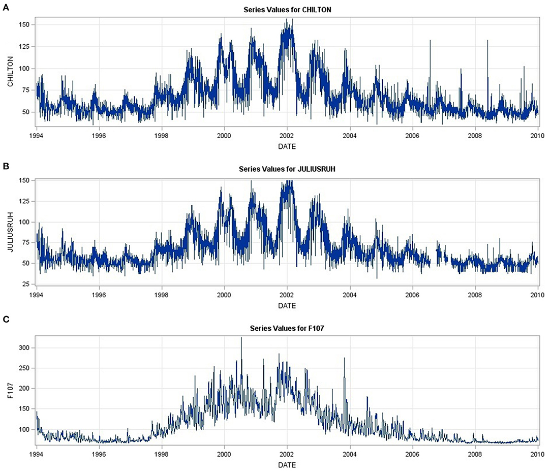
Figure 1. Plot of time-series of critical frequency foF2 (in 0.1 MHz) measured in Chilton (51.5°N, 1.3°W) (A) and Juliusruh (54.6°N, 13.4°W) (B) together with the solar activity index F10.7 recorded during solar cycle 24 (C).
Impact of the incoming energy depends on the actual state of the atmosphere-ionosphere system; hence it may vary with time and location. The important factors determining how the system deposits the incoming energy lay within the atmosphere-ionosphere system of the Earth. So far, the way the ionosphere responds to the solar input is not completely understood. The manner in which solar energy is absorbed by the atmosphere is the subject of large international projects. Recently, projects of the Scientific Committee on Solar-Terrestrial Physics (SCOSTEP), such as Variability of the Sun and Its Terrestrial Impact (VarSIT) (Georgieva and Shiokawa, 2014) focused on the solar impact on the terrestrial atmosphere. An important question that still needs to be answered is the mechanism of the response of the Earth, which is variable and may significantly depend on the atmospheric state of the Earth and its history due to the long memory of the system. Scientific question on how the coupling takes place within the terrestrial atmosphere was one of the important parts of the project, namely, the Role of the Sun and the Middle atmosphere/thermosphere/ionosphere in Climate (ROSMIC) (Lübken et al., 2014). The main goal of the new SCOSTEP program, namely, Predictability of Variable Solar-Terrestrial Coupling (PRESTO) is to improve the predictability of energy flow in the integrated Sun-Earth system on a time scale from a few hours to centuries by promoting international collaborative efforts. Vertical coupling, as an important task, is defined within Pillar 2 (Chang et al., 2020).
Another solar activity variation, the ~27-day solar rotation variation caused by the distribution of solar active regions and coronal holes over the solar disc, is also reflected in the variations of the ionosphere and thermosphere (Lee et al., 2012; Ren et al., 2020). Solar flares are another important solar phenomenon that impacts the ionosphere. Their effects on the ionosphere have broadly been studied (Huba et al., 2005; Liu et al., 2006; Pawlowski and Ridley, 2008; Qian et al., 2011, 2020). Strong solar flares like those that occurred on 6 September 2017 are capable of causing a blackout of radio wave propagation for tens of minutes (Fagundes et al., 2020). Solar flares induced changes in the ionosphere and they also affect Global Navigation Satellite System (GNSS) radio signals and their applications, for example, in positioning (Shagimuratov et al., 2020).
Joint analyses of the solar activity indices and atmospheric parameters cover only several last solar cycles. The longest time-series available are regular measurements of critical frequency foF2. Data records of standard meteorological parameters provide the possibility to detect solar influence as deep as at the ground level. Climatological studies reveal significant solar forcing of the Earth climate based on long-term surface temperature measurements. Historical records of ground-level temperature offer unique opportunities to study the solar influence on the interannual–centennial climate variability (Eddy, 1976; Friis-Christensen and Lassen, 1991; Beer et al., 2000; Scafetta, 2010). The response of the Earth's atmosphere shows significant variability. A large climatological study (Scafetta, 2014) demonstrated that using only one solar index does not capture all the complexities of the solar influences on the atmosphere. At some periods, the atmospheric parameters are positively correlated with the solar activity while in others they are negatively correlated with the solar activity. Different manifestations of solar activity (solar poloidal field and toroidal field) have different impacts on the terrestrial system (Borovsky and Denton, 2006; Georgieva et al., 2006). Changing correlation between the North Atlantic oscillation and the sunspot number during the solar cycle with respect to poloidal and toroidal solar magnetic fields was reported by Georgieva et al. (2012). Analyses of coherency between common period domains in the solar, atmospheric (stratospheric temperature), and ionospheric parameters revealed that atmospheric response varies during the solar cycle and from one cycle to another (Koucká Knížová et al., 2018).
One aspect of investigations of the influence of solar activity on the ionosphere is the utilization of solar activity indices/proxies (Brown et al., 2018), because homogeneous series of satellite measurements of solar ionizing radiation are often not available. Important is the selection of optimum/best solar proxy. In the past, the sunspot number was the most used parameter. Then it was replaced by the F10.7 solar index (solar radio flux at a wavelength of 10.7 cm). Vaishnav et al. (2019) used 12 different solar proxies and found that for variations on time scales, from week-to-week to month-to-month He II followed by Mg II, are the best available solar proxies. Laštovička (2021) found the Mg II index to be the best for year-to-year time scale for foF2. However, these indices are available for a significantly shorter period than F10.7.
In addition to the above coupling, the solar origin also comprises the impact of geomagnetic storms on the ionosphere (Buonsanto, 1999; Danilov, 2013). However, the impact of geomagnetic storms on the ionosphere and upper atmosphere is out of the scope of this paper; it would deserve a long-separated paper.
Despite an extremely high agreement between the general course of solar index F10.7 and ionospheric parameters shown in Figure 1, there is a significant day-to-day variability in the electron concentration. Even when keeping a similar level of incoming solar energy, the evolution of foF2 can show significant variability. Fang et al. (2013) estimated that about half of the observed variability in the ionospheric F2 peak plasma density is related to the lower atmosphere forcing under moderate solar activity and quiet geomagnetic conditions.
Figure 2 shows changes of maximum foF2 on the daily basis (notice August 20 compared to the following days) and in the entire course. Taking into account only the incoming solar radiation, the ionospheric concentration should theoretically depend on the solar zenith with one daily maximum. However, the two-maxima diurnal course is a rather commonly observed case even in the situation of stable and low solar and geomagnetic conditions (Kp < 2 for most of the selected period). Hence the source of the observed variability is identified in the atmospheric waves and their imprints into the ionospheric plasma.
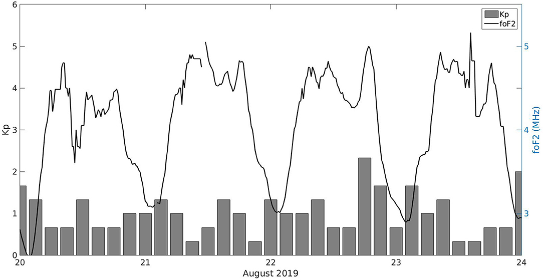
Figure 2. Diurnal course of foF2 (solid line) recorded at Pruhonice observatory on 20–23 August 2019 during geomagnetically low activity (Kp index in gray).
Traveling Ionospheric Disturbances
The variability of the upper atmosphere is seen in fluctuations within the observed data on a wide range of scales. Most of the observed variations are intermittent wave-like oscillations with variable lifetime. Wave-like oscillations with periods of few minutes to ~2 h, called gravity waves (GWs) are permanently present within the atmosphere. They have the potential to propagate through the atmosphere over large distances (vertically and/or horizontally) and carry energy and momentum. Their signatures in the ionospheric plasma are known as traveling ionospheric disturbances (TIDs). TIDs significantly affect electron concentration profiles changing their shape, redistributing the concentration and/or total electron concentration. These effects in turn change the conditions for propagation of electromagnetic signals at all ranges. Ionospheric variability due to TIDs leads to an increase in the uncertainty in the navigation and communication systems.
TIDs are registered practically in all measured parameters at all heights and times. Most common sources of TIDs are considered to be geomagnetic storms, auroral activity (Bristow et al., 1996), and atmospheric waves propagating from lower-lying atmospheric layers. The wave characteristics of TIDs depend on the particular source (Holt et al., 2017). There are many identified sources of the observed ionospheric fluctuations. Among them, meteorological systems, solar terminators, and eclipses are of particular interest. Except for the natural oscillations, the anthropogenic wave-like oscillations attributed to explosions can be detected (Panasenko et al., 2018; Huang et al., 2019 and references therein). According to their period and wave velocity, TIDs can be divided into three groups, such as large-scale TIDs (LSTIDs), medium-scale TIDs (MSTIDs), and rarely studied small-scale TIDs (SSTIDs). Characteristic scales of SSTIDs are less than 10 km according to Swarm measurements (Yin et al., 2019); GWs of similar scales were observed in the mesosphere. MSTIDs have characteristic periods up to 60 min and their horizontal velocities are approximately 100–300 m.s−1. Typical periods of the observed LSTIDs in the ionospheric heights are about 50 min to 3 h with horizontal velocities of 400–1,000 m.s−1. Details about the TIDs can be found in the work of Hocke and Schlegel (1996) or Panasenko et al. (2018).
Coupling and Atmospheric Waves
The ionosphere is permanently changing on a wide range of scales reflecting the variable amount of energy coming from the above and coming from below. The upper atmosphere in midlatitudes is influenced via EUV and X-ray radiation. The heating and photoionization lead to the expansion of the atmosphere and plasma formation. A review paper by Trenberth et al. (2009) provides insight into the energy budget within the atmosphere of the Earth down to the surface and oceans of the Earth. Incoming solar radiation is partly absorbed by atmospheric constituents heating the atmosphere and forming ion pairs, and partly propagates down to the surface and reflects back. Incoming radiant energy may be scattered and reflected by clouds and aerosols or absorbed in the atmosphere. Energy may be stored for some time, transported in various forms, and converted among the different types, giving rise to a rich variety of weather or turbulent phenomena in the atmosphere and oceans. Based on satellite data obtained during 2000–2004, it provides the global annual mean of the energy budget of the Earth (Trenberth et al., 2009). The energy deposited in the low atmosphere significantly contributes to the atmospheric wave generation.
It has been widely accepted that the atmospheric regions are coupled predominantly via vertically propagating waves that transfer energy and momentum over large distances (Yiǧit and Medvedev, 2015; Yiǧit et al., 2016). Due to the conservation of kinetic energy, wave amplitudes grow exponentially with increasing height. The response of the geospace to atmospheric waves generated by the meteorological events, their interaction with the mean flow, and their impact on the ionosphere and their relation to competing thermospheric disturbances generated by energy inputs from above, such as auroral processes at high latitudes were important parts of the SCOSTEP CAWSES-II Project (Oberheide et al., 2015b). Atmospheric waves, particularly the motions of GW, tidal wave (TW), and planetary wave (PW) are persistent wave-like oscillations that are observed in all types of atmospheric data, including neutral wind and temperature, pressure, density, and geopotential height.
Gravity Waves
Under suitable conditions for propagation, initially small perturbation may grow to a large wave oscillation at higher altitudes, where it may affect the environment significantly. Atmospheric waves (that involve tidal, planetary, gravity, and acoustic waves) may directly or indirectly affect winds, temperature, compositional structures, the circulation pattern, neutral and ion species transport, and ionospheric wind dynamo. The first pioneering work which pointed out that atmospheric waves are important for understanding the atmospheric and ionospheric variability, appeared in the 1960's. Experiments conducted by different instrumental techniques recorded irregularities and irregular motions within atmospheric observed parameters. The departures from the model based purely on solar and geomagnetic activity needed an explanation. Hines (1960, 1963, 1965, 1968) interpreted the observed variability in terms of atmospheric GWs propagating through the atmosphere of the Earth. The effects of GW on the ionospheric plasma up to the height of F2 region through photochemical and dynamical processes were proposed later by Hooke (1970b). Hooke (1970a, 1971) used theoretical models to show that resulting effects of GWs can significantly vary in the ionospheric plasma depending not only on the wave properties, but also on the actual ionospheric state and/or the direction of propagation with respect to the incoming solar radiation (Hooke, 1968).
Model studies by Vadas and Fritts (2005), Vadas (2007), Yiǧit et al. (2009), Yiǧit and Medvedev (2010), and Yiǧit et al. (2012) demonstrated gravity-wave propagation through the upper atmosphere of the Earth. Later, Vadas and Nicolls (2012) proved that GWS originating in the tropospheric convection can reach thermospheric heights and significantly affect the profiles of wind and temperature. Atmospheric waves propagate from the lower-lying atmosphere up to the thermosphere either as primary or secondary or even as tertiary waves. The momentum deposited by breaking GWs in the mesosphere and lower thermosphere (MLT) region excites the secondary gravity waves (Vadas et al., 2003, 2018; Vadas and Liu, 2009). Atmospheric wave propagation through the atmosphere depends on the actual state of the background atmosphere. Wind properties affect when and whether particular waves reach the upper atmosphere (Cowling et al., 1971; Fritts and Alexander, 2003; Sun et al., 2007).
Recent results show that not only the secondary but even the tertiary GWs play a role in the thermosphere and ionosphere (Vadas and Becker, 2019). Trinh et al. (2018) reported observation of primary and secondary GW-induced structures in satellite [Sounding of the Atmosphere using Broadband Emission Radiometry (SABER), the Gravity Field and Steady-State Ocean Circulation Explorer (GOCE), and Challenging Minisatellite Payload (CHAMP)] observations. A review paper by Yiǧit and Medvedev (2015) provided the theory of internal atmospheric wave propagation. It focused on the temporal scales of minutes till several days. Works of Laštovička (2006), Smith (2012a), Liu (2016), Yiǧit et al. (2016) provided an overview of lower atmospheric forcing done predominantly via atmospheric waves and proposed mechanisms on how the coupling takes place in the particular atmospheric region. Gathering experimental data, Liu (2016) concluded that lower atmospheric forcing can contribute to the ionosphere and thermosphere variability up to ~35%, especially during solar minima.
Garcia and Solomon (1985) demonstrated the importance of GWs for changes in the chemical composition of the middle atmosphere. The experimental ionospheric study (Williams et al., 1987) discussed the meteorological influences on the ionosphere and interactions during periods of stratospheric warming in the winter of 1983/1984. Shpynev et al. (2019) reported medium-scale wave-like disturbances in the winter ionosphere caused by the atmospheric waves arising in high-speed jet streams in the stratosphere and mesosphere. Fritts and Nastrom (1992) suggested that convective activity in the troposphere is as important a source of GWs for topographic forcing. Collocated satellite observations of concentric acoustic-gravity wave (AGW) type disturbances originated in thunderstorm activity were reported by Yue et al. (2019). Azeem and Barlage (2017) reported the concentric wave features and the extended squall line generated TIDs from convective tropospheric sources. Xu et al. (2019) reported hurricane-generated concentric GWs observed in both the stratosphere and mesosphere from spaceborne satellites and in the ionosphere by the ground-based Global Positioning System (GPS) receivers. Wave-like activity induced in the ionospheric plasma in connection with meteorological frontal systems were reported by Boška and Šauli (2001), Chernigovskaya et al. (2015), Borchevkina et al. (2020), and Koucká Knížová et al. (2020).
Fritts and Alexander (2003) provided an overview of the GW dynamics and effects within the middle atmosphere. It addresses particular GW sources and the corresponding propagation characteristics. A study by Yiǧit and Medvedev (2017) revealed that GWs appreciably impact the mean circulation and cool the thermosphere down by up to 12–18%. It further indicates that the effects of GW depend on the mutual correlation of the diurnal phases of the GW forcing and tides: GWs can either enhance or reduce the tidal amplitude. It has been pointed out recently that the effects of GW during sudden stratospheric warming (SSW) should be considered (Yiǧit and Medvedev, 2016). Model simulation (Liu, 2017) and later experimental SABER observations (Liu et al., 2020) showed that GWs can contribute significantly to the large wind shears at mesopause region heights. The simulated large wind shear peak varies with the season at middle to high latitudes: higher during winter and lower during summer, consistent with the seasonal variation of the mesopause height. Recently Yiǧit et al. (2021) have used the Coupled Middle Atmosphere Thermosphere-2 GCM to study the importance of latitudinal variability in the GW sources for the middle and upper atmosphere.
Pedatella and Liu (2018) implemented atmospheric variability into the model study of the atmosphere and ionosphere system to one particular geomagnetic storm. Involving arbitrary internal atmospheric variability leads to the geomagnetic storm occurring under a different, though climatically similar, atmospheric state for each ensembled member. While large-scale features of the storm were reproduced well, small-scale characteristics of the response were dependent on lower atmosphere variability. Uncertainty may lead to values of typically 20–40%, with localized regions exceeding 100%. Liu et al. (2017) demonstrated long-term cumulative effect of the non-storm corrugations in the prediction of the satellite orbital evolution. Prediction or modeling of the non–storm time thermosphere is important to improve the knowledge of coupling two largely different systems: the magnetosphere-ionosphere-thermosphere (MIT) system on the one side and with the meteorological system in the lower atmosphere.
Park et al. (2014) reported climatology of medium-scale GW activity in the midlatitude and low-latitude thermosphere based on the observations by CHAMP satellite. The important feature is a seasonal variability with higher GW activity during local winter. Park et al. (2014) suggested that the observed waves are secondary GWs generated by the breaking of primary GWs around 90 km altitude. The most recent results by Heale et al. (2020) provided a very complex pattern of the upward propagation of gravity waves with multiple breaking and production of a spectrum of non-primary gravity waves propagating into the thermosphere and ionosphere. Vadas et al. (2003) proposed that the body force that accompanies wave breaking is potentially an important linear mechanism for generating secondary waves that propagate into the mesosphere and lower thermosphere and that the efficiency of this forcing is independent of the latitude. However, spatial and temporal variability/intermittency of a body force is important in determining the properties and associated momentum fluxes of the secondary waves.
The solar terminator (ST) contributes significantly to the regular ionospheric variability. The moving border between sunlit and dark atmosphere separates regions with and without incoming solar energy. In the vicinity of the solar terminator, the atmospheric gas is in a non-equilibrium state with strong gradients in the temperature and density that lead the system into a non-equilibrium state, giving rise to atmospheric irregularities and inhomogeneities (Somsikov, 1995; Somsikov and Ganguly, 1995). ST moves due to the rotation of the Earth. The shape of the terminator curve changes with the seasons (equinox vs. solstice) and shows differences between sunrise and sunset. On the surface, the velocity changes from the equator to the poles. At the equator, the ST moves with supersonic velocity. As the ST moves through the atmosphere, it generates waves that propagate up to ionospheric heights. At first, the ST-induced waves were reported by Chimonas and Hines (1970) and Beer (1973). Theoretical formulations for the wave generation in the atmosphere and ionosphere remain as the subject for many studies, for instance, Beer (1978), Cot and Teitelbaum (1980), and Somsikov (1987, 1995). According to these studies, the sharper the boundary is, the more efficient the source of wave generation will be.
The linear mechanisms of wave generation by ST assume that GWs are excited by the motion of the discontinuity in the values of atmospheric parameters (energy flux, temperature, and electron density). Both the acoustic wave and GW can be radiated in association with supersonic motion in the atmosphere, while only GWs can be emitted from the moving source within the atmosphere with subsonic velocity (Kato et al., 1977). However, in real anisotropic plasma, the generation mechanism is more complicated. The development of instabilities (gradient-radiative, convective, and flow) must be taken into account at ionospheric heights.
Satellite measurements indicate that the amplitudes of ST-induced waves depend on the solar cycle—larger amplitudes can be detected during solar maximum than during solar minimum (Miyoshi et al., 2009). Liu et al. (2009) reported the existence of a prominent phase shift between the ST-induced wave structures in the wind and density fields, and a clear dawn-dusk asymmetry, with more pronounced wave structures at dusk. That corresponds to the theory that in the evening, ST works more effectively in exciting atmospheric waves. Afraimovich (2008) evidenced two types of total electron content (TEC) disturbance associated with ST. Large-scale variations and medium-scale wave packets are space-fixed along the ST line over a distance exceeding 1,600 km. Bespalova et al. (2016) and later Fedorenko et al. (2017) reported regular fluctuations induced by the solar terminator seen with a predominant wave mode moving synchronously with the terminator within the fluctuation of the neutral thermospheric components, O and N2 measured by satellites, such as Dynamic Explorer 2 and Atmosphere Explorer-E.
The source of ST waves detected within the thermospheric heights was attributed to the upward propagating high-order migrating tides generated in the ozone layer by the moving ST (Fujiwara and Miyoshi, 2006; Šauli et al., 2006b; Forbes et al., 2008; Miyoshi et al., 2009). The enhancement of GW activity in the ionospheric plasma during and several hours after sunrise, together with vertically propagating waves, through the ionosphere from a source located at an altitude of 180–220 km were reported by Boška et al. (2003).
Solar eclipses work in a similar way as ST. Moving obscured atmospheric regions were found to be an effective source of atmospheric waves (Somsikov, 1995). Within the eclipsed region, due to temperature drop, pressure decreases over the totality belt, which induces a response in the neutral wind and further the downward flux relative to pressure levels and consequently, molecular diffusion reacts to restore the equilibrium (Rishbeth et al., 1969; Mueller-Wodarg et al., 1998). Fritts and Luo (1993) modeled eclipse-induced wave structures with the source in cooling the ozone layer during the eclipse. Wang et al. (2019) modeled in detail, processes that lead to the observed changes within the ionospheric plasma during the solar eclipse.
Solar eclipses are rare but well-predicted cases. Therefore, campaigns are usually prepared to analyze the effects of the eclipse in detail. However, there are not two exactly identical solar eclipses, and/or occurring during solar and geomagnetic conditions that may allow the study of the solar eclipse-induced effects separately from other sources. Satellite and ground-based measurements revealed AGW structures propagating through the ionosphere (Šauli et al., 2007; Jakowski et al., 2008). Two source regions of the detected solar-eclipse-induced waves were reported by Farges et al. (2003). Šauli et al. (2006a) detected waves with periods of 3–5 min (acoustic mode) and 15–40 min (gravity mode), and identified some modes propagating from the source region located around 200 km height, while other from the source, possibly in the ozone layer. Mošna et al. (2018) analyzed the 2015 solar eclipse and using a combination of different ground methods, detected persistent AGW activity up to the height of 150–250 km with a dominant period of 65 min. Lin et al. (2018) reported solar eclipse-induced waves with periods of 20–30 minutes in the TEC measurements that well-correspond to those derived by the Global Ionosphere-Thermosphere Model (GITM). Large attention has been paid recently to the total solar eclipse that occurred on 21 August 2017 above North America. Experimental studies reported significant changes in all ionospheric F-layer parameters and identified wave-like structures associated with the eclipse by means of both ground-based and space-based equipment (Nayak and Yiǧit, 2018; Verhulst and Stankov, 2018; Yang et al., 2018; Perry et al., 2019; Uma et al., 2020). Mrak et al. (2018) pointed out that the observed wave structures may be attributed to two different sources, such as untangled wave structures emitted by the tropospheric system and solar eclipse-induced wave structures.
Infrasound
Besides GWS, meteorological processes in the troposphere have the potential to generate acoustic waves. Infrasound covers frequencies between the lower limit of human hearing (~20 Hz) and the acoustic cut-off frequency. The acoustic cut-off frequency is of the order of 0.001 Hz; its exact value depends on the temperature and composition and thus changes with height (Davies, 1990). Infrasound is strongly absorbed in the upper atmosphere at heights above 90 km (Georges, 1968; Sutherland and Bass, 2004). The attenuation of the signal depends on its frequency. Generally, lower frequencies are less attenuated at a given altitude. Infrasound observations in the ionosphere concern frequencies lower than 1 Hz (Blanc, 1985). The temperature decrease in the troposphere and in the mesosphere results in infrasound focusing during its upward propagation and, therefore, infrasound can efficiently transfer energy from the lower atmosphere to the ionosphere (Laštovička, 2006). On the other hand, due to the focusing, infrasound waves affect only spatially limited regions in the upper atmosphere above the source; infrasound generated by convective storms was observed in the ionosphere within the radius of 300 km from its tropospheric source (Georges, 1973).
Most of the infrasound sources are sporadic, such as volcanic eruptions, earthquakes, solar eclipses, bolides and meteorites, man-made explosions, supersonic jets, and spacecraft launches. Meteorological activity and ocean waves can be on the global scale considered to be continuous sources of infrasound. Tornadoes, convective storms, weather fronts, mesoscale convective complexes, and airflow over mountains belong to the most efficient meteorological sources of infrasound (Laštovička, 2006; Campus and Christie, 2010). Ionospheric infrasound generated by convective storms in the troposphere was broadly studied in North America in the 1960's and 1970's. Observations of 1–5 min waves in the ionosphere were repeatedly reported during the nearby convective storms (Georges, 1967, 1973; Baker and Davies, 1969; Davies and Jones, 1973; Chimonas and Peltier, 1974; Prasad et al., 1975). Infrasound research was nearly forgotten in the following decade (Laštovička, 2006). The interest was revived in the 1990's, when the Comprehensive Nuclear-Test-Ban Treaty was opened to signature (www.ctbto.org). Recently, the applicability of infrasound for the tomography of the middle atmosphere has been investigated and infrasound seems a promising tool for such types of measurements (Le Pichon et al., 2005, 2006; Blanc et al., 2018). Azeem et al. (2018) observed circular ionospheric disturbances in TEC that propagates radially outward from the center of the storm. Ionospheric infrasound is also excited by earthquakes (see section Seismo–ionospheric effects).
Tides
In general, major forcing on tidal periods in the lower and middle atmosphere results in atmospheric heating due to the absorption of solar radiation by stratospheric ozone and water vapor. The resulting oscillations are reflected in migrating tides, which propagate with the apparent solar motion, which is a function of the local time (Chapman and Lindzen, 1970; Oberheide et al., 2015a). Another part of the tidal motion that depends on the longitude includes non-migrating tides with other generation mechanisms, such as surface topography, geographically variable heat sources, and variation of solar heating with longitude. Compared to migrating tides, the non-migrating tides can propagate eastward or westward with respect to the Sun, or stands alone. Pancheva and Mukhtarov (2011) provided an overview of the global spatial (altitude and latitude) structure, seasonal and interannual variability of the atmospheric tides, and planetary waves derived from the SABER/Thermosphere, Ionosphere, Mesosphere Energetics and Dynamics (TIMED) temperature measurements for full 6 years (January 2002–December 2007). They provide patterns of the wave activity in the stratosphere-mesosphere-lower thermosphere system. Borries et al. (2007) detected standing and traveling wave-like disturbances in the TEC data and interpreted them as signatures of PW.
Using the Whole Atmosphere Community Climate Model (WACCM) and data from SABER/TIMED, Pedatella et al. (2016) concluded that short-term variability of eastward propagating non-migrating diurnal tide with zonal wave number 3 in the mesosphere and lower thermosphere is caused by the combination of changes in troposphere forcing, zonal mean atmosphere, and wave–wave interactions. Using the Kyushu GCM, Miyoshi and Yiǧit (2019) analyzed the impact of small-scale GWs on the semidiurnal tide. Study shows that GW drag significantly decelerates the mean zonal wind in the thermosphere. In particular, the GWs attenuate the migrating semidiurnal solar-tide (SW2) amplitude in the lower thermosphere and modify the lati-tudinal structure of the SW2 above a 150 km height. Jin et al. (2012) reported an enhancement of the semidiurnal tide in the lower thermosphere during the sudden stratospheric warming (SSW) of 2009 and suggested possible mechanisms in the enhancement of its source due to the redistribution of stratospheric ozone and/or change of propagation condition.
Possible generation mechanism of nonlinear interactions between migrating tides and stationary PWs has been discussed by Angelats i Coll and Forbes (2002), Pancheva et al. (2009), and recently by Das et al. (2020), who found that nonlinear interactions are not dominant sources for the generation of non-migrating tides in the middle- and high-latitude winter stratosphere. Smith (2012b) reviewed observations and numerical modeling of the dynamical processes that control the Mesosphere and Lower Thermosphere (MLT) and its variability. The review includes the effects of atmospheric waves as a circulation pattern within the region.
Planetary Waves
On longer time-scales, the differential heating of the Earth's surface due to geography gives rise to the PWs or Rossby waves that form global wind patterns. The resulting air flow affects both horizontal and vertical temperature patterns. It leads to strong pronounced wind structures and forms large planetary scale wave-like structures and jets as a result of a balance between the pressure gradient force and the Coriolis force. PWs cannot propagate directly well above the lower thermosphere (mainly due to atmospheric viscosity). Therefore, they propagate to the F2-region in the ionosphere heights via modulating other upward propagating waves, particularly tides (Laštovička and Šauli, 1999; Pancheva et al., 2003), or via modulation of the ExB drift (Pancheva et al., 1994). Observational data confirm the (indirect) propagation of PWS into the thermosphere (Pancheva et al., 1994, 2003). Takahashi et al. (2005) identified quasi 2- and 4-day period oscillations in the ionospheric F-layer bottom height (h0F) and airglow emission. Planetary wave-type oscillations in the ionosphere occur in bursts of oscillations with a typical duration of four waves for periods around 5 days, of 3.5 waves for periods around 10 days, and no more than three waves for periods around 16 days (Lastovicka et al., 2006). Fagundes et al. (2009) found the influence and modulation of the vertical F-layer post-sunset displacement by traveling planetary wave ionospheric disturbance according to the disturbance phase.
Based on satellite data, Pancheva et al. (2012) demonstrated similarity in the lower thermospheric temperature tides and their corresponding ionospheric signatures and further discussed spatial structures of the ionospheric response. Fang et al. (2013) reported significant longitudinal and day-to-day variations in the ionospheric parameters on simulations with the global ionosphere plasmasphere model driven by the whole atmosphere model winds. In consistent with the observations, they found larger relative variability in the nighttime than in the daytime. Under moderate solar activity and geomagnetically quiet conditions, the perturbations from the lower atmosphere contribute about half of the observed variability in the ionospheric F peak plasma density. Significant day-to-day variability has long been observed in ground-based Fabry-Perot Interferometer wind measurements leading to implementation of the lower-lying atmospheric region into circulation models (Roble, 2000; Siskind et al., 2012, 2014). Zawdie et al. (2020) simulated the day-to-day variability of high frequency (HF) propagation in the bottom side ionosphere using an ionosphere model coupled to a whole atmosphere model driven by the lower atmosphere involving the effects of lower atmospheric weather. They captured part of the observed variability suggesting that the most likely source of this missing variability are low-altitude ion transport terms that are perpendicular to the magnetic field in regions where the motion becomes strongly dominated by ion-neutral collisions.
Sudden Stratospheric Warmings
Sudden stratospheric warmings are winter-time increases in the polar stratospheric temperature. The primary mechanism of SSW origin is the interaction of the planetary waves with the zonal mean flow (Matsuno, 1971). SSWs are divided into two groups, such as major and minor, according to the presence or absence of the high-latitude (60°) zonal wind reversal at the 10 h Pa level. Liu et al. (2010) showed that although the PW activity associated with SSWs is concentrated to high latitudes, the nonlinear interaction between tides and the quasi-stationary planetary wave enhances migrating and nonmigrating tides globally. Numerical simulations by Pedatella and Liu (2013) confirmed the important role of changes in the migrating semidiurnal solar (SW2) and lunar (M2) tides as well as in the westward propagating non-migrating semidiurnal tide with zonal wave number 1 (SW1). Global scale modeling studies Yiǧit and Medvedev (2012) and Yiǧit et al. (2014) of direct gravity wave propagation into the thermosphere during a minor sudden warming showed that GW effects increase in the thermosphere during a minor warming. Eswaraiah et al. (2017) demonstrated the measurements and model simulation of a minor SSW that has the potential to affect the dynamics of the MLT region in a similar manner as major SSW.
Observations demonstrate a strong connection between SSWs and pronounced changes in the ionosphere in the MLT region as well as in the F region (Goncharenko and Zhang, 2008). Analysis of Jicamarca plasma drifts in a large range of heights between 140 and 900 km using Incoherent Scatter Radar data showed a strong connection between stratospheric high-latitude parameters and average morning and afternoon equatorial Ex B drift changes. Ionospheric studies of SSWs predominantly at low latitudes have been performed mainly due to the observation of strong effects of the 2009 SSW on the low latitude ionosphere (Fejer et al., 2010; Goncharenko et al., 2010). Pedatella and Forbes (2010) showed that zonal winds during SSWs play an important role in coupling between the lower atmosphere and ionosphere. Results from the first period of investigations of the ionospheric effects of SSWs were reviewed by Chau et al. (2012). Ionospheric effects of SSWs at low latitudes are longitudinally dependent (Fang et al., 2012; Liu et al., 2019). The effects of Arctic SSWs were observed also in the southern low-latitude ionosphere (de Jesus et al., 2017; Vieira et al., 2017). A strong thermospheric cooling accompanied the January 2009 SSW (Liu et al., 2011a), which is a feature of the typical temperature response to a major SSW. Siddiqui et al. (2018) and Yadav et al. (2019) found that the equatorial ionosphere response to SSW is distinctly different for different phases of the Quasi-Biennial Oscillation (QBO). A strongly enhanced lunar semidiurnal tide plays an important role in the ionospheric effects of SSWs at low latitudes (Fejer et al., 2010; Forbes and Zhang, 2012). Based on the Thermosphere-Ionosphere-Electrodynamics General Circulation Model (TIE-GCM) simulations, Pedatella (2016) concluded that the major SSW forcing is a significant factor strongly modifying the effect of the major geomagnetic storm in the equatorial ionosphere by up to 100% of storm-induced TEC change.
Ionospheric effects of SSWs were broadly studied at low latitudes but much less at middle latitudes. Nayak and Yiǧit (2019) have investigated the effect of the major sudden stratospheric warming (SSW) event of 2009 on the small-scale gravity wave (GW) activity in the ionosphere. Midlatitude investigations of the effects of SSW on the ionosphere bring some light on the ionospheric response (Goncharenko et al., 2013; Liu et al., 2019), but the response is not well-understood yet. Also, minor SSWs, not only major SSWs, are capable of significant modification of the midlatitude ionosphere (Medvedeva and Ratovsky, 2018). In the American sector, the nighttime SSW-induced TEC perturbations in ~55°S−45°N were found to be negative and substantially stronger than daytime perturbations (Goncharenko et al., 2018). Both the Constellation Observing System for Meteorology, Ionosphere, and Climate (COSMIC) observations and Thermosphere Ionosphere Mesosphere Electrodynamics General Circulation Model (TIME-GCM) simulations reveal perturbations in hmF2 at Southern Hemisphere midlatitudes during SSW 2009 and 2013 time periods, which are of ~20–30 km (10–20% variability of the background mean hmF2) (Pedatella and Maute, 2015).
Seismo-Ionospheric Effects
Investigations of ionospheric disturbances triggered by earthquakes started with the pioneering studies that investigated atmospheric and ionospheric response to the great Alaskan earthquake in 1964 (Bolt, 1964; Donn and Posmentier, 1964; Davies and Baker, 1965). Earthquakes and resulting seismic waves lead to the vertical movement of the ground surface that generates infrasound waves propagating nearly vertically upward owing to supersonic speeds of seismic waves. Only long-period infrasound, with periods longer than ~10 s, can reach the ionosphere; the shorter periods (higher frequencies) are significantly damped below the ionosphere. Thus, only waves from strong (M > 7) earthquakes that produce sufficiently long periods are usually detected in the ionosphere, whereas no ionospheric disturbances are observed for weak earthquakes, even for observations above the epicenter (Blanc, 1985; Laštovička et al., 2010).
The coseismic ionospheric disturbances are often studied from the changes induced in the total TEC that can be derived from the observations by networks of dual-frequency receivers of GNSS. Dense networks make it possible to study the propagation of circular coseismic ionospheric disturbances (Calais and Minster, 1995; Heki and Ping, 2005; Liu et al., 2011b). Great attention is paid to the ionospheric signatures produced by tsunamis as there is a potential to use these signatures in early warning systems (Arai et al., 2011; Kakinami et al., 2012). The idea is based on the fact that atmospheric waves propagate faster than tsunami waves (around 200 m/s at deep water). A necessary assumption is that the epicenter is sufficiently far away from the coastline. Correct real-time recognition of a co-tsunami disturbance remains a big challenge due to the complexity of the problem. Lin et al. (2017) modeled a tsunami-like wave packet and studied the impacts on the ionosphere-thermosphere system.
Harrison et al. (2010) proposed a mechanism of increased electrical conductivity of surface layer air before a major earthquake that leads to reduced surface-ionosphere electrical resistance and explained the observed changes in the natural extremely low frequency (ELF) radio noise by DEMETER satellite as earthquake-induced variations. Pulinets and Ouzounov (2011) provided a complete model of Lithosphere–Atmosphere–Ionosphere Coupling (LAIC) that involves processes from tectonics up to ionospheric processes that may help validate the observed ionospheric earthquake precursors.
Coupling Evidences Within Ionospheric Plasma—Experiments in Midlatitudes
Advantage of ground-based stations, compared to satellite measurement, is that they provide sounding on a regular basis for a long time. A large worldwide system of ionosondes and Digisondes has been in operation since the inception of the International Geophysical Year (IGY); hence the time series from vertical ionospheric sounding covers a longer period than satellite missions. The length of the dataset is appreciated in trend analyses. The ionosonde measures reflections of electromagnetic waves of defined frequencies transmitted vertically into the ionosphere and reflected to the receiver [details of ionospheric sounding can be found in Davies (1990)]. The output is height-frequency characteristics (called ionogram) of the ionosphere, from where the essential property of the ionospheric plasma can be derived. Critical frequency foF2 is one of the representative parameters. Critical frequency (i.e., maximum plasma frequency in the layer) is proportional to the maximum electron concentration that is usually located in the F2 layer. Critical frequency foF2 represents the most suitable parameter for longer time-scale analyses. The echo in the receiver depends on the actual state of the ionosphere and its properties with respect to the sounding wave. When the wave is reflected on the horizontal isodensity plane, the recorded ionogram is clear with well-defined reflection traces. When the ionosphere is disturbed or tilted, the registered echo is spread due to off-vertical signals. Interpretation of ionograms can be found in the study by Wakai et al. (1987). Except regular ionogram measurement/sounding, the Digisondes perform drift measurements. Hence, Digisonde data consists of ionospheric parameters derived from ionograms and Sky maps (Reinisch, 1996; Reinisch et al., 1998, 2005). Detailed description can be found also on the web page of https://ulcar.uml.edu/digisonde.html. Besides Digisonde data, we further use data from multi-point continuous Doppler sounding (CDS), and a description of the method can be found on http://www.ufa.cas.cz/files/OHA/M_Doppler_system.pdf. Kouba and Chum (2018) demonstrated the efficiency of Digisonde-based drift measurement together with CDS on fixed frequency for the study of dynamics of the ionosphere. Satellite measurements are another independent source of data.
Three-Dimensional Analysis
Variability within the ionospheric plasma is often observed in the wave-like form, especially in the TIDs. Chum et al. (2012a), using the multi-point CDS system, showed that MSTIDs usually propagated with horizontal components of phase velocity directed against the neutral winds in the middle latitude ionosphere, which corresponds with the dominant horizontal component of GW propagation. Consequently, the azimuths of GW propagation also exhibited seasonal and diurnal dependence; TIDs mostly propagated toward the equator in winter and toward the pole in summer. Specifically, the observations were performed over the Czech Republic and South Africa. The propagation against neutral winds is consistent with previous theoretical studies (Cowling et al., 1971; Sun et al., 2007; Vadas, 2007). Recently, Chum and Podolská (2018) performed a 3D analysis based on the observations by multi-frequency and multi-point Doppler sounding system operating in the Czech Republic (reflection points of the sounding electromagnetic signals are separated both horizontally and vertically) and showed that MSTIDs/GWs propagated with wave vectors directed obliquely downwards. It directly follows from the dispersion relation (Hines, 1960; Davies, 1990; Vadas, 2007) that obliquely downward-pointing wave vectors (phase velocity vectors) mean oblique upward propagation of group velocity and wave energy of GWs. Figure 3 shows the phase velocity vectors of the GWs in 3D, while the GWs were analyzed over a one-year period from July 2014 to June 2015. Since the Doppler receiver does not distinguish between the ordinary and extraordinary mode, the obtained results are shown for an assumption of receiving ordinary (L-O) and extraordinary (R-X) modes separately. There are only minor differences between the results obtained for the L-O and R-X modes. The reflection heights that are necessary for the 3D analysis of propagation (Chum and Podolská, 2018) were obtained from a nearby Digisonde located at Pruhonice. There are two main horizontal directions of propagation. The GWs propagated roughly south-eastward during the daytime in winter and roughly north-westward around sunset in summer (Figures 3A,B). It should be noted that 3D analysis was often not possible because of low cross-correlation of the signals observed for different transmitter-receiver pairs or because of the lack of signals at some frequency, for example, due to low foF2. Consequently, the data coverage in the day-of-year-daytime plane was relatively rare (Chum et al., 2021). The vertical cross-sections of phase velocities displayed in Figures 3C,D for the L-O and R-X modes, respectively, demonstrate that the analyzed GWs propagated mostly with phase velocities (wave vectors) directed obliquely downward, and are consistent with the source of energy below.
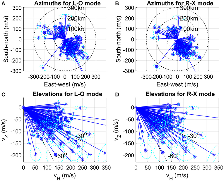
Figure 3. Observed phase vector velocities in the horizontal plane obtained under the assumption of receiving ordinary L-O mode (A) and extraordinary R-X mode (B) and the observed phase vector velocities in the vertical cross-section obtained under the assumption of receiving ordinary L-O mode (C) and extraordinary R-X mode (D). Cyan circles show estimated uncertainties.
Long-Term Data
As mentioned, most of the observed variability is manifested in wave-like structures from seconds up to solar cycle scales or secular variations. Figure 1, in the previous part, demonstrates similarity in the dominant course of the critical frequency for two distant ionospheric stations (Panels A and B). Figure 4 shows the decomposition of the original foF2 from Chilton and Juliusruh stations. The original time series Ot (Panels A and D) were split into dominant trend TCt (Panels B and E), and irregularities It (Panels C and F), where Ot = TCt + St + It. Here irregularities mean irregular components in time series decomposition, which are the residues of the analyzed process. They can be interpreted as turbulences within the ionosphere. We applied the additive decomposition method with centered moving average adjustment for all cyclic Ct and seasonal St components. The trend-cycle TCt is the component of the original time series that represents variations of low frequency. The Hodrick-Prescott filter (Brockwell and Davis, 1991) which decomposes the trend-cycle component TCt into the trend component and cycle component in an additive form was used. The irregular components It from the original data were separated as non-adjusted. The results of decomposition (seasonal adjustment, trend cycle plot, and irregular plot) are displayed in the sub-panels for each station. A smaller value assigns less significance to the cycle (0 value implies no cycle component). The time series decomposition performed in SAS 9.4TM (SAS Institute Inc. 2012. SAS OnlineDoc® 9.4. Cary, NC: SAS Institute Inc., https://support.sas.com/documentation/94/) was used.
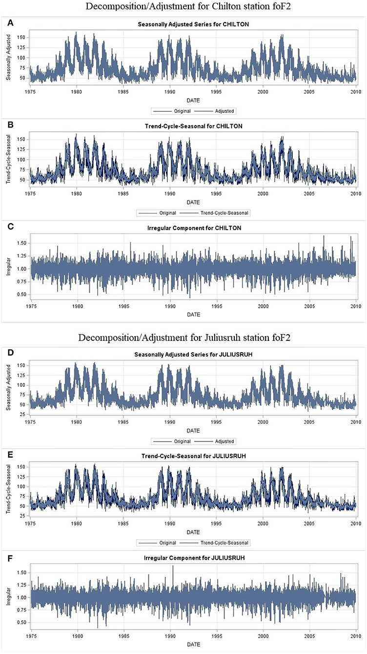
Figure 4. Decomposition of critical frequency foF2 time series (in 0.1 MHz) for Chilton and Juliusruh, 1994–2010. The seasonal adjustment (A,D), trend cycle plot (B,E), and irregular plot (C,F) are displayed in the sub-panels for each station.
The dominant course of critical frequency is formed by regular solar forcing. The remaining irregular part consists of both lower atmosphere forcing and irregular solar impact. From the stability F-test of maximum percentage difference [difference in the original series and the centered moving average of the sum of the values of the irregular components exceeded 3.0% (Findley et al., 1990)], it is apparent that the irregular component is not stable. It is slightly larger during solar maxima (here, beginning in years 1979, 1989, and 2001) with respect to solar minima (here beginning in years 1976, 1986, 1996, and 2008). However, relative deviation during solar minima may exceed the deviation values during solar maxima, which indicates the importance of considering the irregular component.
Figure 5 shows the foF2 time series and its interaction with the simply differenced series of F10.7. The following panels visualize the foF2 time series on the Chilton station recorded in the data set from 1975–2010 and its interaction with the simply differentiated series, F10.7 during the same time period. The series plot in Panel (A), the correlation Panel (B), the seasonal adjustment Panel (C), and the standardized cross-correlation function plot in Panel (D) are displayed. The autocorrelation function (ACF) coefficients of correlation between a time series and its lagged values, partial autocorrelation function (PACF) explain the partial correlation between the series and lags of itself, inverse autocorrelation functions (IACF) and white noise probabilities (Box et al., 2008) are rendered in the correlation Panel (C) in Figure 5. If either the ACF or a PACF between observations of n lags apart is statistically significant, the autocorrelation is included in the AR model (Box et al., 2008). The partial autocorrelation plot in Figure 5B suggests that the data are modeled with a first-order autoregressive model, AR (1). The significance of the autocorrelation is evaluated from the 95% confidence intervals plotted in Panel (B). Test sets of lags for the first n lags for the analyzed standardized cross-correlation function (CCF) (Box et al., 2008) are shown in Panel (C). The lags evaluated from the 95% confidence interval are marked with a darker blue area, and the 90% confidence intervals are marked with the lighter blue area. In Figure 5D shows visualized cross-series plots of F10.7 and foF2 time series. The F10.7 time series is normalized to the mean values of foF2. At the time intervals where the normed series, F10.7 (standardized to the average value foF2 series) has a larger variance, their mutual correlation is lower. Such a situation is clearly visible during all three maxima solar cycles in the observed period.
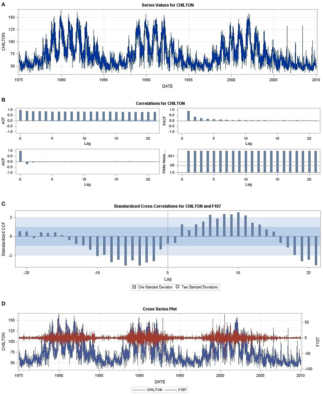
Figure 5. Cross-correlation analyses for F10.7 and foF2 (0.1 MHz) at midlatitude station Chilton recorded in 1975-2010 cover three solar cycles (21–23). [Normed F10.7 cross-correlation series plot in (J.s−1.m−2.Hz1), and all correlation and cross-correlation functions are dimensionless [1]]. The series plot (A), the correlation (B), the seasonal adjustment (C), and standardized cross-correlation function plot in (D) are displayed.
Long-Term Trends
Long-term trends in the upper atmosphere and ionosphere are also in some sense influenced by the vertical coupling in the atmosphere-ionosphere system. Their main driver, even though not the only driver, is the increasing concentration of anthropogenic carbon dioxide (CO2) in the atmosphere (Laštovička et al., 2012). The origin of this process increases its concentration near the surface, which propagates upward by various processes of vertical coupling (vertical transport and mixing). Both, satellite observations [TIMED/SABER and Atmospheric Chemistry Experiment (ACE)/Fourier Transform Spectrometer (FTS)] and models reveal up to ~90 km the same trend of increasing CO2 concentration as that at the surface, whereas near the E-layer maximum, the observational trend is even somewhat stronger but its difference from the model and surface trends is only marginally statistically significant (Rezac et al., 2018). Another way of vertical coupling in the area of long-term trends in the upper atmosphere and ionosphere is the impact in the changes of the stratospheric ozone, which has well been observed at the ionospheric E-region heights, particularly in the neutral atmosphere density but which is undetectable at F2 region heights (Laštovička et al., 2012). Trends in the upper atmosphere and ionosphere are also affected by trends/changes in the activity of atmospheric waves coming from the lower atmosphere, but this effect is not yet well-understood and various observational results do not provide a consistent pattern; in fact, the only clear information is that such effects appear to be clearly regionally dependent (Laštovička, 2017). Thus, vertical coupling plays a crucial role in the long-term changes in the climate of the upper atmosphere and ionosphere.
Influence of Tropospheric Mesoscale Systems
It is assumed that the effects of the neutral atmosphere on the ionosphere have limits in their spatial extent. Koucká Knížová et al. (2015) investigated the evolution of a correlation between stations with distance for long time series of foF2. They identified the “break point” at 10° in longitude and/or Earth's distance of ~1,000 km as shown in Figures 6A,B. Analyzed foF2 time series from European ionospheric stations covered the time span of several solar cycles. Signals were split into mean courses and fluctuations, and correlations of raw, mean, and fluctuation time series were computed. On both panels in Figure 6, an extremely high correlation is visible not only for the time series of mean and raw courses, but also for fluctuations up to the break point. Since the scale of ~1,000 km corresponds to the typical sizes of mesoscale tropospheric systems, this finding supports a connection between the lower atmosphere and the F2 region.
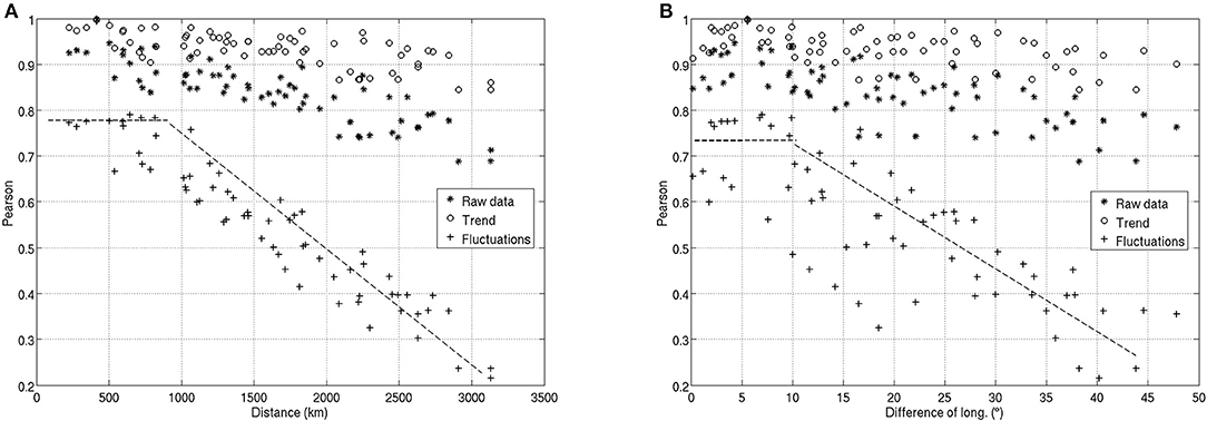
Figure 6. Pearson linear correlations between foF2 at different stations as a function of distance between them with respect to surface distance (A) and longitudinal difference (B) [adopted from Koucká Knížová et al. (2015)].
Large Mesoscale Systems
Large cyclonal systems are recognized to be an efficient source of AGWs that are able to propagate upward and reach the ionospheric heights. Our study detected significant increase of wave-like activity at ionospheric heights following immediately after the cross of the frontal system above the ionospheric station (Boška and Šauli, 2001; Šauli and Boška, 2001; Sindelarova et al., 2009; Koucká Knížová et al., 2020). We expect to observe propagating atmospheric waves associated with the tropospheric cyclonal system at heights of the ionosphere due to their ability to alter reflection conditions within the ionosphere. The spread of F ionograms was reported to be associated with AGWs (Bowman, 1981, 1988, 1990; Dyson et al., 1995; Bencze and Bakki, 2002; Xiao et al., 2009; Yu et al., 2016).
The spread of F ionogram depicted in Figure 7A may result from the GW launched by the meteorological system causing an off-vertical echo. Further, the direction, amplitude, and Doppler shift of the arriving echoes are presented in a form of directogram as shown in Figure 7B. Figure 7B, shows that the Digisonde detects a significantly higher number of moving points during the day of the frontal passage above the station compared to the preceding and following days.
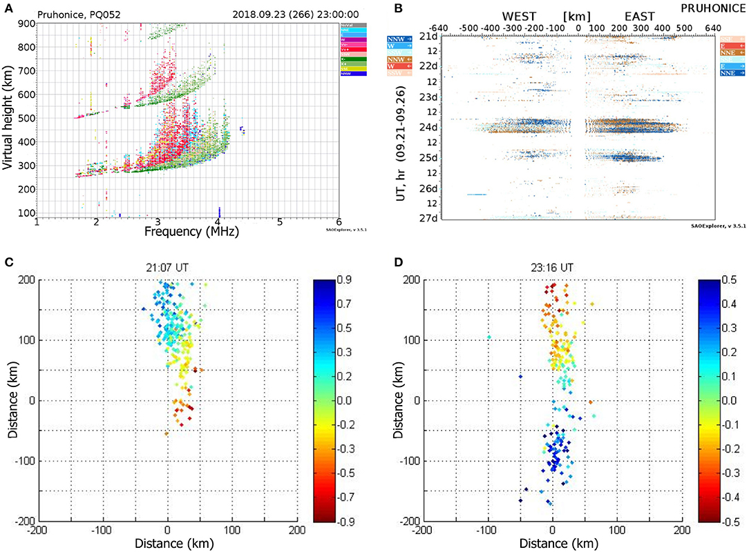
Figure 7. Upper panels show spread of F ionogram recorded after the frontal system passage (A), and directograms measured for several consequent days (B) before and after Fabienne Cyclone. Bottom panels demonstrate SkyMaps recorded after the Fabienne passage over ionosonde station at 21:01 UTC (C) and at 23:16 UTC (D). Blue and red colors denote the Doppler shift of the moving plasma (horizontal projection of plasma flow toward and away from the observer, respectively). (A,B) Were adopted from Koucká Knížová et al. (2020).
Digisonde measures plasma motion near the foF2 frequency. The output is a SkyMap (Reinisch et al., 1998). Method of SkyMap evaluation was described by Kouba and Koucká Knížová (2012). It has been demonstrated that such disturbances within the ionosphere may lead to high-quality measurements of plasma drifts using Digisonde. When the Digisonde registers a high number of off-vertical reflection points that can be approximated by a well-defined vector, it is possible to derive representative drift characteristics. Plots in Figure 7 show the situation when isodensity planes are not perfectly horizontal. The registered off-vertical reflections occur on tilts formed by gravity waves.
Figures 7C,D show examples of the characteristics of SkyMap. Left SkyMap (Panel C) is recorded 16 min after the ionogram measurement in Panel (A), while the right SkyMap (Panel D) is recorded with about 2 h delay. Both maps correspond well to the horizontal flow with a high number of reflection points. From the SkyMaps, it is evident that ionospheric plasma moves in different directions with different velocities. Left SkyMap indicates plasma flow in the east-southeast direction while the right one shows the motion northward. Using discontinuous deformation analysis (DDA) (Kozlov and Paznukhov, 2008) method, the characteristic velocities of detected structures moving above the observational points are as follows:
vN = -114 ± 20 m.s−1, vE = 242 ±5 0 m.s−1, vz = 16 ± 7 m.s−1 at 21:07 UT and vN=70 ± 6 m.s−1,
vE = 10 ± 60 m.s−1, vz = −12 ± 2 m.s−1 at 23:16 UT.
The large differences in the direction and speed of the ionospheric plasma in a relatively short time interval demonstrate the severity of the impact of the tropospheric storm.
Continuous Doppler sounding represents another source of data for detailed analyses of meteorological storm influence. In Central Europe, observations of ionospheric infrasound of meteorological origin are rather rare. Wave periods of 2–5 min superimposed on GWs were observed in the F region mainly during extreme weather events in European conditions like extremely severe convective storms in July 2005 and cyclone Kirill in January 2007 (Sindelarova et al., 2009).
Figure 8A presents observations of ionospheric infrasound on 6 November 2012. Wave periods of 2–6 min were observed at altitudes of 250–330 km from 00 to 04 Coordinated Universal Time (UTC). The waves propagated upward with vertical velocities close to the local sound speed derived from the MSISE90 model outputs (the observed vertical velocity measured ~600–900 m/s, and local sound speed according to the model measured 790–830 m/s). The observed infrasound is most probably of tropospheric origin. During the analyzed time period, a cold front passed through Czechia from the north-west. Ahead of the cold front, a strong gusty wind was registered for about 45 min. This was followed by short-term heavy rain from cumulus clouds. During the subsequent 30 min, the air pressure moved up gradually, the temperature at the height of 2 m dropped sharply by about 3°C, resulting in a postfrontal reduction in the wind speed and precipitation.
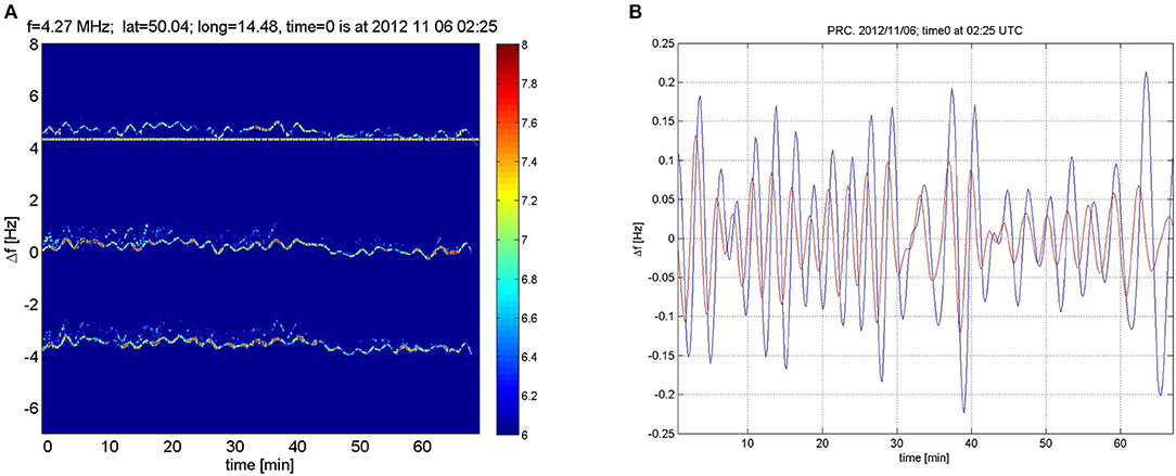
Figure 8. (A) Shows the Doppler shift spectrogram recorded on 6 November 2012 from 2:25 to 3:35 UTC. Reflection height of the 4.27 MHz Doppler sounding wave was 280–330 km. Recordings at the three sounding paths are shown; from top to bottom: Pruhonice–Prague, Panska Ves–Prague, and Dlouha Louka–Prague. (B) Presents recordings at the sounding path: Pruhonice–Prague (PRC) on 6 November 2012 from 02:25 to 03:32 UTC. The Doppler frequency shift, Δf is proportional to the change of the phase path of the sounding radio wave and to the frequency of the wave. Red line represents measurements at the sounding frequency of 3.59 MHz; the Doppler sounding wave reflects at heights of 250–300 km. Blue line represents measurements at the sounding frequency of 4.27 MHz; the Doppler sounding wave reflects at heights of 280–330 km. Filtered signals in the period range of 2–6 min are shown.
Infrasound measurements at two frequencies were available for the 6 November 2012 event. Figure 8B shows the delayed infrasound arrivals at higher ionospheric altitudes, which allow for the estimation of the vertical component of the velocity of propagation of infrasound.
Sporadic E Layer
The sporadic E layers (Es) are relatively thin sheets of increased electron concentration largely exceeding the ionization in background E layer plasma. The main source of the ionized material are meteors which disintegrate in the MLT region and increase the concentration of metallic ions (mainly Mg+, Fe+, Na+, and Ca+). The widely accepted wind-shear theory explains that the Es layers formed at middle latitudes as a result of wind with relatively different velocities (thus a wind-shear) in the presence of proper configuration of magnetic field lead to the accumulation of electrically charged particles in a thin layer. Therefore, the behavior of Es layers is largely controlled by the neutral atmosphere as it modulates the zonal and meridional winds in the E region. The tidal activity is well seen as a periodic descent of the Es layer (Figure 9). Local and seasonal dependence of neutral wind shear is an important factor in determining the dependence of the Es layer occurrence rate on geographical distribution and seasonal variation (Chu et al., 2014; Shinagawa et al., 2017). Jacobi and Arras (2019) found good correspondence between the radar derived wind shear and Es phases for the semidiurnal, terdiurnal, and quarterdiurnal tidal components. General knowledge of the midlatitude sporadic-E phenomenon was reviewed by Haldoupis (2012).
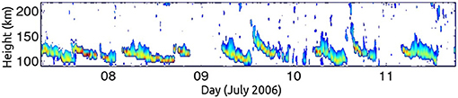
Figure 9. Five consequent days of sporadic E height-time intensity during July 2006. The method of Haldoupis et al. (2006) was applied to the Pruhonice Digisonde data.
The Es layer exhibits strong tidal and PW domain variability. Our experimental high-sampling campaigns show that the dominant tidal mode with the central period of 24 h significantly varies in the range of 22–26 h (Šauli and Bourdillon, 2008). The proposed mechanism lay in the small perturbation of the Es height by the PW. The E layer is moved up and down at the PW frequency, producing a Doppler shift and a variation in the central period around 24 h. In the present case (Figure 10), the 24-h spectral mode is modulated by PW with a period of about 4 days in both critical frequency and height of Es layer. Additionally, modulation of the central mode of foEs by PW with a period of 6.5 days is well seen during the entire campaign.
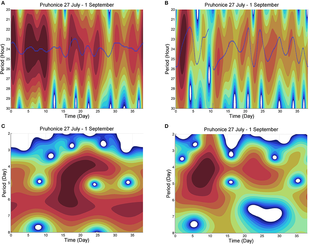
Figure 10. Diurnal mode detected in high-sampling measurements of foEs (A) and hEs (B) data in campaign 2004. The central mode varies from 22 to 26 h in both cases. Bottom panels [foEs in left, (C) and hEs in right, (D)] show wavelet power spectrum (WPS) of the central mode with significant planetary domain modulation. WPS spectrum is normalized (1 - dark red) to the maximum value at the particular scale. The upper (A,B) were published in Šauli and Bourdillon (2008).
Further, our high sampling observations of Es variability revealed an important link between stratospheric temperature and both foEs and hEs data. Joint analyses of stratospheric (wind and temperature) and Es parameters identified common coherent wave bursts in spectra on periods close to Eigen-periods of the terrestrial atmosphere (Mošna and Koucká Knížová, 2012; Mošna et al., 2015).
Impact of SSW on the Ionosphere
Our study of the European midlatitude ionosphere response to three major SSWs, which occurred under deep solar activity at minimum conditions on January 2009, February 2018, and December 2018 to January 2019, reveals an interesting feature. All three SSW events were accompanied by a remarkable increase in foF2, as illustrated by Figure 11 for Pruhonice station, just in the interval of temperature maximum and between the two maxima of zonal wind reversal. Similar increase in electron concentration was observed for average TEC over Europe. Yet, we do not have any explanation for these observations. These three major SSW events were accompanied by much higher occurrence frequency of ionospheric spread conditions, probably as a consequence of enhanced atmospheric wave activity and related formation of ionospheric irregularities.
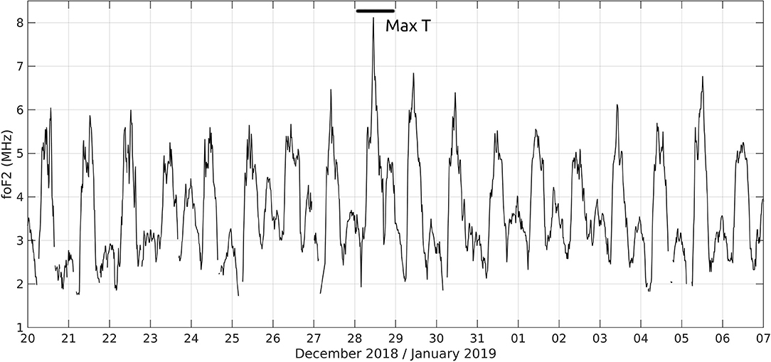
Figure 11. Evolution of foF2, Pruhonice, February 2018. The most dominant feature is a short-time increase of maximum daytime values on 17 February, in the interval of SSW temperature maximum.
Seismo-Ionospheric Effects
Chum et al. (2012b) observed coseismic infrasound over the Czech Republic in the form of relatively compact wave packets (several minutes long) that were associated with individual seismic wave packets of P, S, SS, and Rayleigh waves triggered by the devastating M9 Tohoku earthquake on 11 March 2011. The observations were done at about 9,000 km distance from the epicenter. The time delays between the observations of seismic waves on the ground and coseismic infrasound in the ionosphere were consistent with (quasi)vertical propagation, which is a consequence of supersonic propagation of seismic waves. The waveforms on the ground and ionosphere were similar. A different situation might be observed at intermediate and short distances from the strong earthquakes. In that case, the amplitudes of infrasound waves in the upper atmosphere are so large that the nonlinear phenomena start playing an important role. The non-linear phenomena might lead to significant differences between the spectra observed on the ground and in the upper atmosphere, which cannot be explained by the linear approach, even if the attenuation of higher frequencies owing to viscosity and thermal conductivity is considered. Especially at short distances, the non-linear phenomena might lead to the formation of the N-shaped pulse that resembles a shock wave. Chum et al. (2016) and Chum et al. (2018) showed that the coseismic plasma/air particle velocities derived from CDS were consistent with nonlinear numerical simulation of infrasound wave propagation, considering the viscous atmosphere and boundary condition determined by seismic data for close and intermediate distances from the epicenter by analyzing the M8.3 Chilean earthquake on 16 September 2015 and the M7.8 Nepal earthquake on 25 April 2015. Figure 12 shows the vertical velocity of ground surface movement measured in Tucuman at about 800 km horizontal distance from the epicenter of the earthquake on 16 September 2015 (Figure 12A) and corresponding Doppler shift time series recorded in Tucuman at the height of about 200 km (Figure 12B). Figure 12 documents that fluctuations of air particles/plasma in the thermosphere/ionosphere had completely different waveforms than fluctuations of the ground surface. The difference between waveforms at the ground and waveforms observed in the ionosphere can be explained by non-linear effects that take place in the upper atmosphere owing to large amplitudes of infrasound waves (Chum et al., 2016).
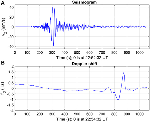
Figure 12. Measured ground surface vertical velocity (A) and corresponding ionospheric fluctuations (B) in Tucuman on 16 September 2015.
Effects of Solar Eclipse
Solar eclipses are rare but well-predicted events. In Central Europe, we had an opportunity to observe several partial solar eclipses. Their effects were reported in the studies by Šauli et al. (2006a), Šauli et al. (2007), Jakowski et al. (2008), and Mošna et al. (2018). An exceptional case occurred on 11 August 1999 when the coverage of solar disk reached 98%, during uniform solar disk, steady solar wind, and in quiet magnetospheric conditions. Hence, fluctuations in the ionosphere mainly consist of the signatures of the ionospheric responses to the solar eclipse. Fast sampling rate campaign (1-min repetition time) was performed by ionosonde. Such a high sampling allowed us to study both acoustic and gravity modes of AGW. Besides that, sounding the entire electron concentration profile permits to extract wave parameters of propagating waves with non-zero vertical components. Applying the wavelet-based toolbox for AGW detection as described by Šauli et al. (2006a) and Šauli et al. (2007), we identified both AW and GWs generated during and immediately after the solar eclipse. Our results reveal asymmetry in the wave activity with respect to occultation and recovery phases of the eclipse. More wave-like activity was registered during the initial phase. Use of wavelets help to untangle particular wave structures, trace them through a height range visible for ionosonde and characterize them in terms of the time of occurrence, period, wave vector, packet, and phase velocities. Figure 13A shows detected acoustic structure developed within the ionospheric plasma during the initial phase of the solar eclipse. Wave properties indicate that acoustic wave-like structure with the period of ~4 min originates at the transition region between ionospheric F1 and F2 layers located around 200 km of height. Wave structures propagate upward and downward through the ionosphere. Detection of the acoustic wave within the ionosonde data was possible only due to high sampling (1-min) measurement. Figures 13B,C present two GW structures identified during and after the eclipse. The first gravity structure occurred in the initial phase of the eclipse and similarly, the acoustic structure propagated upward and downward from the source region close to 200 km height. Second gravity wave structure originated below the ionospheric heights and reached the ionosphere after the recovery phase. Figure 13 demonstrates that solar eclipse impacts significantly the atmosphere and is an effective source for the generation of both AW and GW within ionospheric heights and GWs in the lower-lying atmosphere.
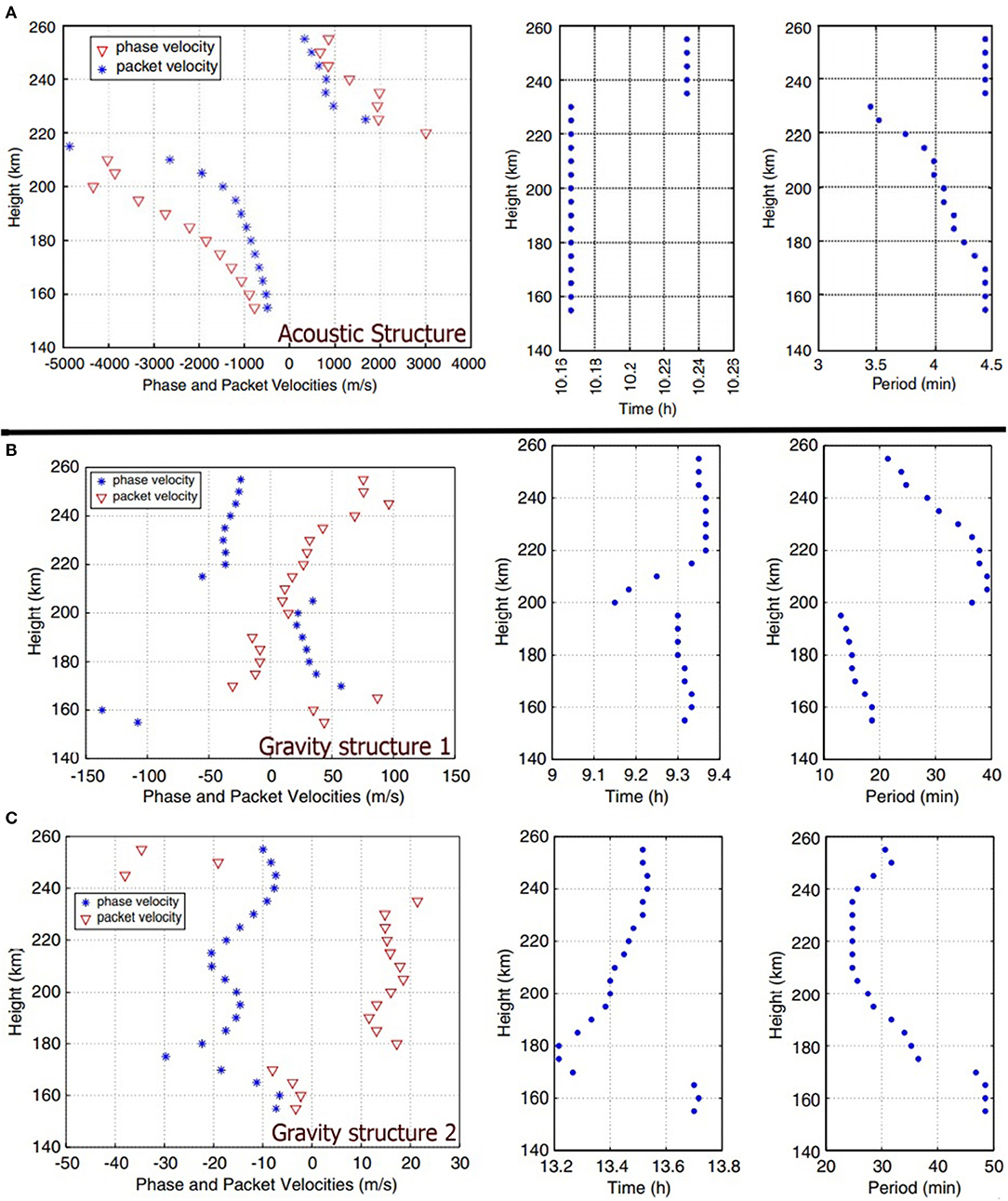
Figure 13. (A) Shows vertical components (phase and packet velocity) of acoustic wave (AW) detected during the solar eclipse of 1999 and its occurrence time and dominant period. (B,C) Are the same as (A), but for the two structures of gravity waves [adopted from Šauli et al. (2006a)].
After the replacement of ionosonde, variability in ionospheric plasma-related solar eclipses were later observed only by Digisonde. Digisonde does not allow as high sampling rate as the ionosonde due to different principles of measurements. Nevertheless, it can be used to monitor wave activity. The sequence of 3 days of ionograms with high temporal resolution up to 5 min was used to visualize the virtual height of the ionospheric plasma during the solar eclipse on 3 January, 2011. Figure 14 shows the results of the adapted method by Haldoupis et al. (2006) for the Digisonde data from Pruhonice station. Quasi-periodic changes in the virtual height of the ionospheric plasma with plasma frequency of 3–4 MHz start up after the first contact (left vertical line in Figure 14B) and persist for more than 4 h after the fourth contact (right vertical line in Figure 14B). This observation confirms that the wave activity triggered by the instability of ionospheric plasma due to rapid change in the absorbed solar energy persists several hours after the end of the disruption (Mošna et al., 2018).
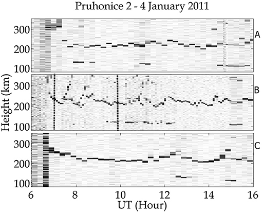
Figure 14. Reflection (virtual) height of sounding waves in the frequency range of 3–4 MHz for 3 consequent days 2–4 January 2011. Oscillation of the reflection height clearly demonstrates wave activity in the ionosphere measured 1 day before (A) the day of the solar eclipse [first and fourth contacts are denoted by vertical lines, (B)], and 1 day after the eclipse (C).
Planetary Wave Signature Within Vertical Plasma Drifts
As mentioned in the previous section, large tropospheric mesoscale systems are considered as an important source of atmospheric waves propagating effectively up to ionospheric heights. The observed ionospheric disturbances can be caused by primary or secondary waves. Their ability to reach the ionospheric heights depends on the actual state of the whole atmosphere. The activity of all atmospheric waves shows seasonal variability. Seasonal changes in the wave-like activity within the ionospheric plasma are well seen in the modulation of the plasma drifts.
Plasma drift data measured by Digisonde DPS 4 collected during 2006 represents measurements under relatively low solar and geomagnetic activity conditions. The ionosphere was rather stably forced from above with only a few short and limited episodes of higher geomagnetic activity. Figure 15A demonstrates a typical diurnal course for each day of the year. The technique for drift data retrieval was described by Kouba and Koucká Knížová (2016). Typical or quiet time vertical components of the plasma drift display a morning negative peak and an evening peak. Besides these two dominant features, rather irregular structures are developed on the mean diurnal course.
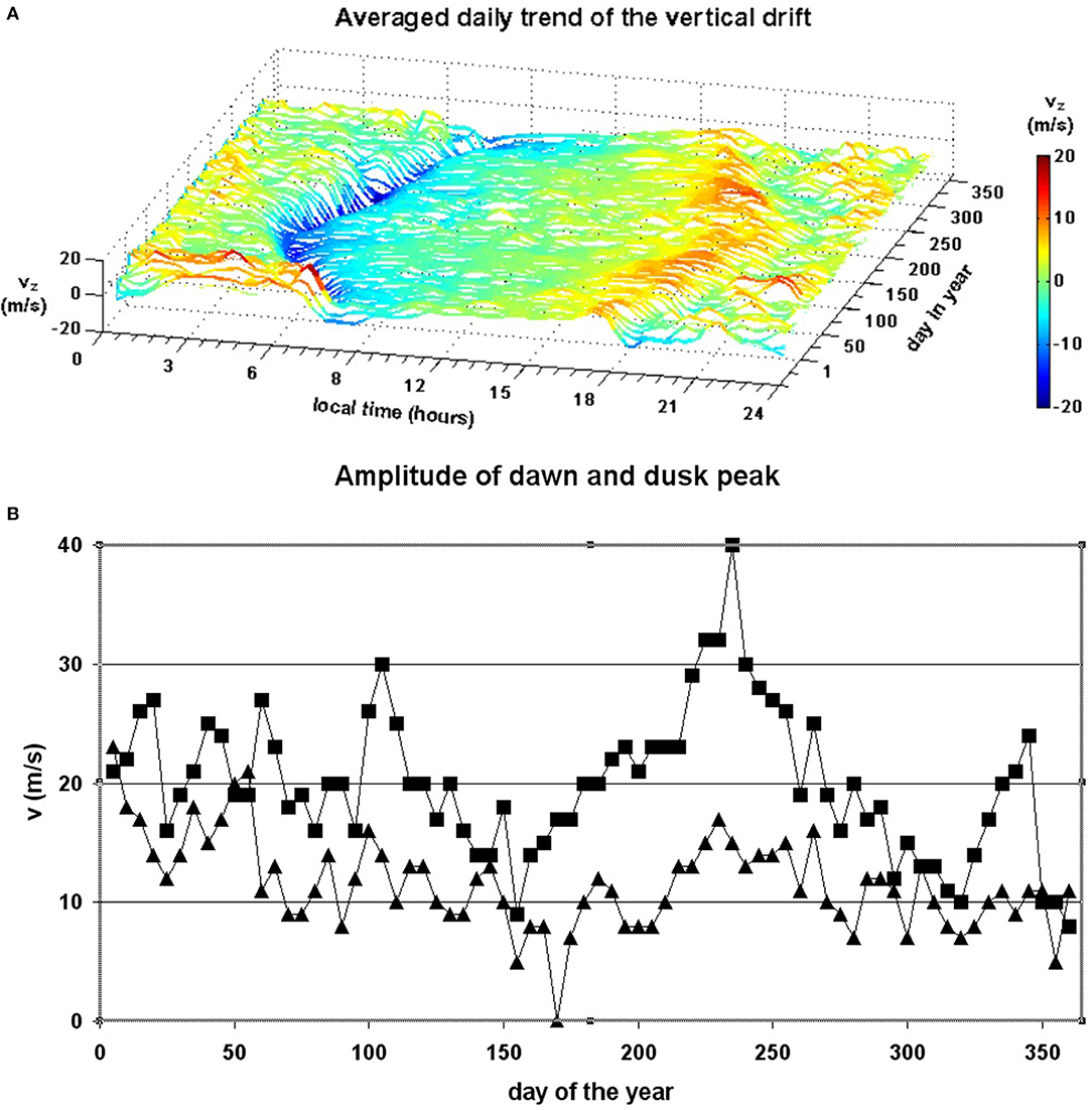
Figure 15. (A) Demonstrates the vertical component of the plasma drift velocity over 2006 as observed at Pruhonice station. (B) Shows the seasonal course of peak values, squares - dawn peak, triangles - dusk peak, year 2006 [according to Kouba and Koucká Knížová (2016)].
Separated plots of the diurnal morning and evening peaks in Figure 15B indicate different behaviors during particular seasons. Larger variability in the period range of several days (corresponding to the domain of the planetary waves) is observed during the winter months. For vertical drift velocities during summer months, it is characteristic of a rather smooth increase in absolute values with maximum close to autumn equinox, when the absolute values start to gradually decrease and show an increase in the variability.
Concluding Remarks
The atmosphere-ionosphere system of the Earth is a very complex region with mutual interactions of neutral and charged particles. The importance of the lower-lying atmosphere is a subject of broad scientific interest and recently, it has been addressed within the activity of large international projects in the frame of the International Association of Geomagnetism and Aeronomy (IAGA) or The Scientific Committee on Solar-Terrestrial Physics (SCOSTEP). Despite the extensive theoretical, modeling, and experimental research, the coupling phenomena in the atmosphere are not yet fully understood and many questions remain to be answered.
Most of the observed variabilities within ionospheric plasma are detected in wave-like forms that overlap on a wide range of space and time scales. On one side, the ionosphere data reflect solar forcing on a wide range of periods, from secular changes, periods connected to solar cycle, seasonal, daily to short-time periods connected to actual solar activity, and properties of solar wind. The ionospheric changes forced “from above” are simultaneously complicated by the neutral atmosphere activity which results in a very complex system which needs detailed analyses for better description of changes in the ionospheric parameters.
The first part of the paper brings a general overview of current understanding of atmosphere–ionosphere coupling. In the second part, we focus on experimental evidence of coupling as they are observed in ground-based measurements by instruments operated by the Institute of Atmospheric Physics, Czech Academy of Sciences. Quality of obtained data confirms the efficiency and significance of techniques based on radio wave reflection even during the satellite era. In this paper we focus on detection, identification, and attribution of the observed ionospheric variability to a particular source.
We demonstrate the influence of large meteorological mesoscale systems on a short time scale. The tropospheric impact is well seen in the changes of ionospheric departures from horizontal stratification, significant plasma flow shears and increase of the speed of horizontal plasma drifts, and detection of infrasound waves within CDS measurements after the passage of the frontal system above the observational point. On longer scales, we show the behavior of correlation coefficient between foF2 fluctuations with respect to the station distance. Extremely high correlation of the fluctuations up to the station distance of ~1,000 km indicate the common origin of the observed fluctuations and supports the idea that the ionosphere is directly influenced by structures with sizes ~1,000 km corresponding to the typical size of mesoscale tropospheric systems.
By means of the CDS system, we present the detection of GWs (3D method) and show two main horizontal directions of propagation with the prevailing direction of the wave vector aiming obliquely downward (i.e., the source of energy is below). Detection of the ionospheric response on M9 Tohoku earthquake (9,000 km distance) shows that the ionospheric signal can be detected on very large distances from the epicenter. The presence of AGWs is also reported as a consequence of solar eclipse events. In particular cases, we analyzed their dominant periods, and phase and packet velocity vectors. In the examples of Es layer data and plasma drift data, we confirm the tidal and planetary wave activity in the E region. We show planetary wave modulation of diurnal mode seen in both variabilities of height and critical frequency of the Es layer. Using the plasma drift data, we show changes in the planetary wave activity throughout the year.
Changes in the F layer ionization have been reported during recent SSW events using the Digisonde and GPS TEC measurement. Short-time and well-defined increase in electron concentration in the F region was observed on days corresponding to the increase in stratospheric temperature and/or the change in the direction of the zonal wind. While the effects of the SSW on the ionosphere in lower latitudes have been broadly shown, the SSW forcing of the ionosphere in middle latitudes has much less been studied.
The presented ionospheric ground-based sounding methods provide good quality of data, which significantly contribute to the understanding of the ionosphere–neutral atmosphere coupling. The main benefits include long-time series of data, relatively dense temporal sampling, and fixed location of the instruments. The latter is a particularly important fact if compared to satellite measurements.
Data Availability Statement
The datasets presented in this study can be found in online repositories. The names of the repository/repositories and accession number(s) can be found at: https://ulcar.uml.edu/digisonde.html; http://datacenter.ufa.cas.cz/archive/.
Author Contributions
PK analyzed Digisonde data (meteorological influence, SE, and Es), performed analyses, made interpretation, prepared review part, and wrote the first draft of the paper. ZM analyzed the Digisonde data (SSW events, SE, and Es) and performed analyses. JL reviewed, made trend analysis, and interpretation. DK operated Digisonde, prepared campaigns, analyzed Digisonde data (drifts), and made interpretation. KPod prepared long-term data analyses, made interpretation, analyzed CDS, and made 3D analysis. KPot collected material for review part, made meteorological analyses, and interpretation. TŠ analyzed CDS data and made interpretation. JC developed 3D analysis of GW propagation, analyzed CDS data, and contributed by the part related to coseismic infrasound. JR prepared CDS and Digisonde data. All authors contributed to the article and approved the submitted version.
Funding
The work of JC, KPod, and JR were supported by the Grant 18-01969S from the Czech Science Foundation.
Conflict of Interest
The authors declare that the research was conducted in the absence of any commercial or financial relationships that could be construed as a potential conflict of interest.
References
Afraimovich, E. L. (2008). First GPS-TEC evidence of wave structure excited by solar terminator. Earth Planet Sp. 60, 895–900. doi: 10.1186/BF03352843
Angelats i Coll, M., and Forbes, J. M. (2002). Nonlinear interactions in the upper atmosphere: the s = 1 and s = 3 nonmigrating semidiurnal tides. J. Geophys. Res. 107:900179. doi: 10.1029/2001JA900179
Arai, N., Iwakuni, M., Watada, S., Imanishi, Y., Murayama, T., and Nogami, M. (2011). Atmospheric boundary waves excited by the tsunami generation related to the 2011 great Tohoku-Oki earthquake. Geophys. Res. Lett. 38:L00G18. doi: 10.1029/2011GL049146
Azeem, I., and Barlage, M. (2017). Atmosphere-ionosphere coupling from convectively generated gravity waves. Adv. Space Res. 61, 1931–1941. doi: 10.1016/j.asr.2017.09.029
Azeem, I., Walterscheid, R. L., and Crowley, G. (2018). Investigation of acoustic waves in the ionosphere generated by a deep convection system using distributed networks of GPS receivers and numerical modeling. Geophys. Res. Lett. 45, 8014–8021. doi: 10.1029/2018GL078107
Baker, D. M., and Davies, K. (1969). F2-region acoustic waves from severe weather. J. Atmos. Terr. Phys. 31, 1345–1352. doi: 10.1016/0021-9169(69)90118-4
Beer, J., Mende, W., and Stellmacher, R. (2000). The role of the sun in climate forcing. Quat. Sci. Rev. 19, 403–415. doi: 10.1016/S0277-3791(99)00072-4
Beer, T. (1973). Supersonic generation of atmospheric waves. Nature 242, 34–34. doi: 10.1038/242034a0
Beer, T. (1978). On atmospheric wave generation by the terminator. Planet. Space Sci. 26, 185–188. doi: 10.1016/0032-0633(78)90017-X
Bencze, P., and Bakki, P. (2002). On the origin of mid-latitude spread-F. Acta Geod. Geoph. Hung. 37, 409–417. doi: 10.1556/AGeod.37.2002.4.4
Bespalova, A. V., Fedorenko, A. K., Cheremnykh, O. K., and Zhuk, I. T. (2016). Satellite observations of wave disturbances caused by moving solar terminator. J. Atmos. Terr. Phys. 140, 79–85. doi: 10.1016/j.jastp.2016.02.012
Blanc, E. (1985). Observations in the upper atmosphere of infrasonic waves from natural or artificial sources: a summary. Ann. Geophys. 3, 673–687.
Blanc, E., Ceranna, L., Hauchecorne, A., Charlton-Perez, A. J., Marchetti, E., Evers, L. G., et al. (2018). Toward an improved representation of middle atmospheric dynamics thanks to the ARISE project. Surv. Geophys. 39, 171–225. doi: 10.1007/s10712-017-9444-0
Bolt, B. A. (1964). Seismic air waves from the great 1964 Alaskan earthquake. Nature 202, 1095–1096. doi: 10.1038/2021095a0
Borchevkina, O., Karpov, I., and Karpov, M. (2020). Meteorological storm influence on the ionosphere parameters. Atmosphere 11:1017. doi: 10.3390/atmos11091017
Borovsky, J. E., and Denton, M. H. (2006). Differences between CME-driven storms and CIRdriven storms. J. Geophys. Res. 111:A07S08. doi: 10.1029/2005JA011447
Borries, C, Jakowski, N., Jacobi, Ch, Hoffmann, P., and Pogoreltsev, A. (2007). Spectral analysis of planetary waves seen in the ionospheric total electron content (TEC): first results using GPS differential TEC and stratospheric analyses. J. Atmos. Terr. Phys. 69, 2442–2451. doi: 10.1016/j.jastp.2007.02.004
Boška, J., and Šauli, P. (2001). Observations of gravity waves of meteorological origin in the F-Region. Phys. Chem. Earth C 26, 425–428. doi: 10.1016/S1464-1917(01)00024-1
Boška, J., Šauli, P., Altadill, D., Sole, J. G., and Alberca, L.F. (2003). Diurnal variation of gravity wave activity at midlatitudes in the ionospheric F region. Stud. Geophys. Geod. 47, 579–586. doi: 10.1023/A:1024763618505
Bowman, G. G. (1981). The nature of ionospheric spread-F irregularities in mid-latitude regions. J. Atmos. Terr. Phys. 43, 65–79. doi: 10.1016/0021-9169(81)90010-6
Bowman, G. G. (1988). Small-scale stratifications associated with daytime travelling ionospheric disturbances in mid-latitude regions. Ann. Geophys. 6, 187–194.
Bowman, G. G. (1990). A review of some recent work on mid-latitude spread-F occurrence as detected by ionosondes. J. Geomag. Geoelectr. 42, 109–138. doi: 10.5636/jgg.42.109
Box, G. E. P., Jenkins, G. M., Reinsel, G. C., and Ljung, G. M. (2008). Time Series Analysis: Forecasting and Control. Oxford: Wiley-Blackwell. doi: 10.1002/9781118619193
Bristow, W. A., Greenwald, R. A., and Villain, J. P. (1996). On the seasonal dependence of medium-scale atmospheric gravity waves in the upper atmosphere at high latitudes. J. Geophys. Res. Space Phys. 101, 15685–15699 doi: 10.1029/96JA01010
Brockwell, P. J., and Davis, R. A. (1991). Time Series: Theory and Methods. New York: Springer. doi: 10.1007/978-1-4419-0320-4
Brown, S., Bilitza, D., and Yiǧit, E. (2018). Ionosonde-based indices for improved representation of solar cycle variation in the International Reference Ionosphere model. J. Atmos. Sol-Terr. Phys. 171, 137–146. doi: 10.1016/j.jastp.2017.08.022
Buonsanto, M. J. (1999). Ionospheric storms—a review. Space Sci. Rev. 88, 563–601. doi: 10.1023/A:1005107532631
Calais, E., and Minster, J. B. (1995). GPS detection of ionospheric perturbations following the January 17 1994, Northridge earthquake. Geophys. Res. Lett. 22, 1045–1048. doi: 10.1029/95GL00168
Campus, P., and Christie, D. R. (2010). “Worldwide observations of infrasonic waves,” in Infrasound Monitoring for Atmospheric Studies, eds A. Le Pichon, E. Blanc, and A. Hauchecorne (Dordrecht: Springer Netherlands), 185234–118.
Chang, L. C., Pallamraju, D., and Pedatella, N. M. (2020). Pillar 2: space weather and Earth's atmosphere. SCOSTEP/PRESTO Newsletter 22, 4–5.
Chapman, S., and Lindzen, R. S. (1970). Atmospheric Tides: Thermal and Gravitational. Dordrecht, Holland: D. Reidel Publishing Co.
Chau, J. L., Goncharenko, L. P., Fejer, B. G., and Liu, H. L. (2012). Equatorial and low latitude ionospheric effects during sudden stratospheric warming events. Space Sci. Rev. 168, 385–417. doi: 10.1007/s11214-011-9797-5
Chernigovskaya, M. A., Shpynev, B. G., and Ratovsky, K. G. (2015). Meteorological effects of ionospheric disturbances from vertical radio sounding data. J. Atmos. Sol. Terr. Phys. 136, 235–243. doi: 10.1016/j.jastp.2015.07.006
Chimonas, G., and Hines, C. O. (1970). Atmospheric gravity waves induced by a solar eclipse. J. Geophys. Res. 75, 875–875. doi: 10.1029/JA075i004p00875
Chimonas, G., and Peltier, W. R. (1974). On severe storm acoustic signals observed at ionospheric heights. J. Atmos. Terr. Phys. 36, 821–828. doi: 10.1016/0021-9169(74)90027-0
Chu, Y. H., Wang, C. Y., Wu, K. H., Chen, K. T., Tzeng, K. J., Su, C. L., et al. (2014). Morphology of sporadic E layer retrieved from COSMIC GPS radio occultation measurements: wind shear theory examination. J. Geophys. Res. Space Phys. 119, 2117–2136. doi: 10.1002/2013JA019437
Chum, J., Athieno, R., Baše, J., Burešov,á, D., Hruška, F., Laštovička, J., et al. (2012a). Statistical investigation of horizontal propagation of gravity waves in the ionosphere over Europe and South Africa. J. Geophys. Res. 117:A03312. doi: 10.1029/2011JA017161
Chum, J., Cabrera, M. A., Mošna, Z., Fagre, M., Baše, J., and Fišer, J. (2016). Nonlinear acoustic waves in the viscous thermosphere and ionosphere above earthquake. J. Geophys. Res. Space Physics 121, 12126–12137. doi: 10.1002/2016JA023450
Chum, J., Hruska, F., Zednik, J., and Lastovicka, J. (2012b). Ionospheric disturbances (infrasound waves) over the Czech Republic excited by the 2011 Tohoku earthquake. J. Geophys. Res. 117:A08319. doi: 10.1029/2012JA017767
Chum, J., Liu, J.-Y., Podolská, K., and Šindelárová, T. (2018). Infrasound in the ionosphere from earthquakes and typhoons. J. Atmos. Sol.Terr. Phys. 171, 72–82. doi: 10.1016/j.jastp.2017.07.022
Chum, J., and Podolská, K. (2018). 3D analysis of GW propagation in the ionosphere. Geophys. Res. Lett. 45, 11562–11571. doi: 10.1029/2018GL079695
Chum, J., Podolská, K., Rusz, J., Baše, J., and Tedoradze, N. (2021). Statistical investigation of gravity wave characteristics in the ionosphere. Earth Planets Space 73:60. doi: 10.1186/s40623-021-01379-3
Cot, C., and Teitelbaum, H. (1980). Generation of gravity waves by inhomogeneous heating of the atmosphere. J. Atmos. Terr. Phys. 42, 877–883. doi: 10.1016/0021-9169(80)90092-6
Cowling, D. H., Webb, H. D., and Yeh, K. C. (1971). Group rays of internal gravity waves in a wind-stratified atmosphere. J. Geophys. Res. 76, 213–220. doi: 10.1029/JA076i001p00213
Danilov, A. D. (2013). Ionospheric F-region response to geomagnetic disturbances. Adv. Space Res. 52, 343–366. doi: 10.1016/j.asr.2013.04.019
Das, U., Ward, W. E., Pan, C. J., and Das, S. K. (2020). Migrating and non-migrating tides observed in the stratosphere from FORMOSAT-3/COSMIC temperature retrievals. Ann. Geophys. 38, 421–435. doi: 10.5194/angeo-38-421-2020
Davies, K., and Baker, D. M. (1965). Ionospheric effects observed around the time of the Alaskan earthquake of March 28, 1964. J. Geophys. Res. 70, 2251–2253. doi: 10.1029/JZ070i009p02251
Davies, K., and Jones, T. B. (1973). Acoustic waves in the ionospheric F2-region produced by severe thunderstorms. J. Atmos. Terr. Phys. 35, 1737–1744. doi: 10.1016/0021-9169(73)90052-4
de Jesus, R., Batista, I. S., Jonah, O. F., Abreu, A. J., Fagundes, P. R., Venkatesh, K., et al. (2017). An investigation of the ionospheric disturbances due to the 2014 sudden stratospheric warming events over Brazilian sector. J. Geophys. Res. Space Phys. 122, 11698–11715. doi: 10.1002/2017JA024560
Donn, W. L., and Posmentier, E. S. (1964). Ground-coupled air waves from the great Alaskan earthquake. J. Geophys. Res. 69, 5357–5361. doi: 10.1029/JZ069i024p05357
Dyson, P. L., Johnston, D. L., and Scali, J. L. (1995). Observations of gravity waves associated with mid-latitude spread-F. Adv. Space Res. 16, 113–116. doi: 10.1016/0273-1177(95)00179-I
Emmert, J. T. (2015). Thermospheric mass density: a review. Adv. Space Res. 56, 773–824. doi: 10.1016/j.asr.2015.05.038
Emmert, J. T., Warren, H. P., Segerman, A. M., Byers, J. M., and Picone, J. M. (2017). Propagation of atmospheric density errors to satellite orbits. Adv. Space Res. 59, 147–165. doi: 10.1016/j.asr.2016.07.036
Eswaraiah, S., Kim, Y. H., Liu, H., Venkat Ratnam, M., and Lee, J. (2017). Do minor sudden stratospheric warmings in the Southern Hemisphere (SH) impact coupling between stratosphere and mesosphere–lower thermosphere (MLT) like major warmings? Earth Plan. Space 69:119. doi: 10.1186/s40623-017-0704-5
Fagundes, P. R., Bittencourt, J. A., Abalde, J. R., Sahai, Y., Bolzan, M. J. A., Pillat, V. G., et al. (2009). F layer postsunset height rise due to electric field prereversal enhancement: 1. Traveling planetary wave ionospheric disturbance effects. J. Geophys. Res. 114:A12321. doi: 10.1029/2009JA014390
Fagundes, P. R., Pezzopane, M., Habarulema, J. B., Venkatesh, K., Dias, M. A. L., Tardelli, A., et al. (2020). Ionospheric disturbances in a large area of the terrestrial globe by two strong solar flares of September 6, 2017, the strongest space weather events in the last decade. Adv. Space Res. 66, 1775–1791. doi: 10.1016/j.asr.2020.06.032
Fang, T.-W., Akmaev, R., Fuller-Rowell, T., Wu, F., Maruyama, N., and Millward, G. (2013). Longitudinal and day-to-day variability in the ionosphere from lower atmosphere tidal forcing. Geophys. Res. Lett. 40, 2523–2528. doi: 10.1002/grl.50550
Fang, T. W., Fuller-Rowell, T., Akmaev, R., Wu, F., Wang, H., and Anderson, D. (2012). Longitudinal variation of ionospheric vertical drifts during the 2009 sudden stratospheric warming. J. Geophys. Res. 117:A03324. doi: 10.1029/2011JA017348
Farges, T., Le Pichon, A., Blanc, E., Perez, S., and Alcoverro, B. (2003). Response of the lower atmosphere and ionosphere to the eclipse of August 11, 1999. J. Atmos. Sol. Terr. Phys. 65, 717–726. doi: 10.1016/S1364-6826(03)00078-6
Fedorenko, A. K., Bespalova, A. V., Zhuk, I. T., and Kryuchkov, E. I. (2017). Latitude variability of acoustic-gravity waves in the upper atmosphere based on satellite data. Geomagn. Aeron. 57, 471–481. doi: 10.1134/S0016793217030057
Fejer, B. G., Olson, M. E., Chau, J. L., Stolle, C., Lühr, H., Goncharenko, L. P., et al. (2010). Lunar-dependent equatorial ionospheric electrodynamic effects during sudden stratospheric warmings. J. Geophys. Res. 115:A00G03. doi: 10.1029/2010JA015273
Findley, D. F., Monsell, B. C., Shulman, H. B., and Pugh, M. G. (1990). Sliding spans diagnostics for seasonal and related adjustments. J. Am. Statist. Assoc. 85, 345–355. doi: 10.1080/01621459.1990.10476207
Forbes, J. M., Bruinsma, S. L., Doornbos, E., and Zhang, X. (2016). Gravity wave-induced variability of the middle thermosphere. J. Geophys. Res. Space Phys. 121, 6914–6923. doi: 10.1002/2016JA022923
Forbes, J. M., Bruinsma, S. L., Miyoshi, Y., and Fujiwara, H. (2008). A solar terminator wave in thermosphere neutral densities measured by the CHAMP satellite. Geophys. Res. Lett. 35:L14802. doi: 10.1029/2008GL034075
Forbes, J. M., and Zhang, X. (2012). Lunar tide amplification during the January 2009 stratosphere warming event: observations and theory. J. Geophys. Res. 117:A12312. doi: 10.1029/2012JA017963
Friis-Christensen, E., and Lassen, K. (1991). Length of the solar cycle: an indicator of solar activity closely associated with climate. Science 254, 698–700. doi: 10.1126/science.254.5032.698
Fritts, D. C., and Alexander, M. J. (2003). Gravity wave dynamics and effects in the middle atmosphere. Rev. Geophys. 41:1003. doi: 10.1029/2001RG000106
Fritts, D. C., and Luo, Z. (1993). Gravity wave forcing in the middle atmosphere due to reduced ozone heating during a solar eclipse. J. Geophys. Res. 98, 3011–3021. doi: 10.1029/92JD02391
Fritts, D. C., and Nastrom, G. D. (1992). Sources of mesoscale variability of gravity waves, 2. Frontal, convective, and jet-stream excitation. J. Atmos. Sci. 49, 111–127. doi: 10.1175/1520-0469(1992)049<0111:SOMVOG>2.0.CO;2
Fujiwara, H., and Miyoshi, Y. (2006), Characteristics of the large-scale traveling atmospheric disturbances during geomagnetically quiet disturbed periods simulated by a whole atmosphere general circulation model. Geophys. Res. Lett. 33:L20108. doi: 10.1029/2006GL027103s
Garcia, R. R., and Solomon, S. (1985). The effect of breaking gravity waves on the dynamics and chemical composition of the mesosphere and lower thermosphere. J. Geophys. Res. Atmos. 90, 3850–3868. doi: 10.1029/JD090iD02p03850
Georges, T. M. (1967). ESSA Technical Report IER 57-ITSA 54. Ionospheric Effects of Atmospheric Waves. Boulder, USA: Institute for Telecommunication Sciences and Aeronomy.
Georges, T. M. (1968). HF Doppler studies of travelling ionospheric disturbances. J. Atmos. Terr. Phys. 30, 735–746. doi: 10.1016/S0021-9169(68)80029-7
Georges, T. M. (1973). Infrasound from convective storms: examining the evidence. Rev. Geophys. 11, 571–594. doi: 10.1029/RG011i003p00571
Georgieva, K., Kirov, B., and Gavruseva, E. (2006). Geoeffectiveness of different solar drivers, and long term variations of the correlation between sunspot and geomagnetic activity. Phys. Chem. Earth 31, 81–87. doi: 10.1016/j.pce.2005.03.003
Georgieva, K., Kirov, B., Koucka Knizova, P., Mosna, Z., Kouba, D., and Asenovska, Y. (2012). Solar influences on atmospheric circulation. J. Atm. Solar-Terrestrial Phys. 90–91, 15–25. doi: 10.1016/j.jastp.2012.05.010
Georgieva, K., and Shiokawa, K. (2014). Introducing VarSITI variability of the sun and its terrestrial impact. VarSITI Newslett. 1, 1–2.
Goncharenko, L., and Zhang, S.-R. (2008). Ionospheric signatures of sudden stratospheric warming: ion temperature at middle latitude. Geophys. Res. Lett. 35:L21103. doi: 10.1029/2008GL035684
Goncharenko, L. P., Coster, A. J., Chau, J. L., and Valladares, C. E. (2010). Impact of sudden stratospheric warmings on equatorial ionization anomaly. J. Geophys. Res. 115:A00G07. doi: 10.1029/2010JA015400
Goncharenko, L. P., Coster, A. J., Zhang, S. R., Erickson, P. J., Benkovitch, L., et al. (2018). Deep ionospheric hole created by sudden stratospheric warming in the nighttime ionosphere. J. Geophys. Res. Space Phys. 123, 7621–7633. doi: 10.1029/2018JA025541
Goncharenko, L. P., Hsu, V. W., Brum, C. G. M., Zhang, S. R., and Fentzke, J. T. (2013). Wave signatures in the midlatitude ionosphere during a sudden stratospheric warming of January 2010. J. Geophys. Res. Space Phys. 118, 472–487. doi: 10.1029/2012JA018251
Haldoupis, C. (2012). Midlatitude sporadic E. A typical paradigm of atmosphere-ionosphere coupling. Space Sci. Rev. 168, 441–461. doi: 10.1007/s11214-011-9786-8
Haldoupis, C., Meek, C., Christakis, N., Pancheva, D., and Bourdillon, A. (2006). Ionogram height–time–intensity observations of descending sporadic E layers at mid-latitude. J. Atmos. Sol.-Terr. Phys. 68, 539–557. doi: 10.1016/j.jastp.2005.03.020
Harrison, R. G., Aplin, K. L., and Rycroft, M. J. (2010). Atmospheric electricity coupling between earthquake regions and the ionosphere. J. Atmos. Sol.-Terr. Phys. 72, 376–381. doi: 10.1016/j.jastp.2009.12.004
Heale, C. J., Snively, J. B., Bossert, K., Vadas, S. L., Hoffmann, L., Dörnbrack, A., et al. (2020). Secondary gravity waves generated by breaking mountain waves over Eur. J. Geophys. Res. Atmos. 125:e2019JD031662. doi: 10.1029/2019JD031662
Heki, K., and Ping, J. (2005). Directivity and apparent velocity of the coseismic ionospheric disturbances observed with a dense GPS array. Earth Planet. Sci. Lett. 236, 845–855. doi: 10.1016/j.epsl.2005.06.010
Hines, C. O. (1960). Internal atmospheric gravity waves at ionospheric heights. Can. J. Phys. 38, 1441–1481. doi: 10.1139/p60-150
Hines, C. O. (1963). The upper atmosphere in motion. Q. J. Roy. Meteorol. Soc. 89, 14–93. doi: 10.1002/qj.49708937902
Hines, C. O. (1965). Dynamical heating of the upper atmosphere. J. Geophys. Res. 70, 177–183. doi: 10.1029/JZ070i001p00177
Hines, C. O. (1968). Some consequences of gravity-wave critical layers in the upper atmosphere. J. Atmos. Terr. Phys. 30, 837–843. doi: 10.1016/S0021-9169(68)80035-2
Hocke, K., and Schlegel, K. (1996). A review of atmospheric gravity waves and travelling ionospheric disturbances: 1982–1995. Ann. Geophys. 14, 917–940. doi: 10.1007/s00585-996-0917-6
Holt, L. A., Alexander, M. L., Coy, L., Liu, C., Molod, A., Putman, W., et al. (2017). An evaluation of gravity waves and gravity wave sources in the Southern Hemisphere in a 7 km global climate simulation. Q J R Meteorol Soc. (2017) 143, 2481–2495. doi: 10.1002/qj.3101
Hooke, W. (1968). Ionospheric irregularities produced by internal atmospheric gravity waves. J. Atmos. Terr. Phys. 30, 795–823. doi: 10.1016/S0021-9169(68)80033-9
Hooke, W. (1970a). The ionospheric response to internal gravity waves, 1. The F2 region response. J. Geophys. Res. 75, 5535–5544. doi: 10.1029/JA075i028p05535
Hooke, W. (1970b). Ionospheric response to internal gravity waves, 3. Changes in the densities of the different ion species. J. Geophys. Res. 75, 7239–7243. doi: 10.1029/JA075i034p07239
Hooke, W. (1971). Quasi-stagnation levels in the ion motion induced by internal atmospheric gravity waves at ionospheric heights. J. Geophys. Res. 76, 248–250. doi: 10.1029/JA076i001p00248
Huang, C. Y., Helmboldt, J. F., Park, J., Pedersen, T. R., and Willemann, R. (2019). Ionospheric detection of explosive events. Rev. Geophys. 57, 78–105. doi: 10.1029/2017RG000594
Huba, J. D., Warren, H. P., Joyce, G., Pi, X., Iijima, B., and Coker, C. (2005). Global response of the low-latitude to midlatitude ionosphere due to the Bastille Day flare. Geophys. Res. Lett. 32:L15103. doi: 10.1029/2005GL023291
Jacobi, C., and Arras, C. (2019). Tidal wind shear observed by meteor radar and comparison with sporadic E occurrence rates based on GPS radio occultation observations. Adv. Radio Sci. 17, 213–224. doi: 10.5194/ars-17-213-2019
Jakowski, N., Stankov, S., Wilken, V., Borries, C., Altadill, D., Chum, J., et al. (2008). Ionospheric behavior over Europe during the solar eclipse of 3 October 2005. J. Atmos. Sol. Terr. Phys. 70, 836–853. doi: 10.1016/j.jastp.2007.02.016
Jin, H., Miyoshi, Y., Pancheva, D., Mukhtarov, P., Fujiwara, H., and Shinagawa, H. (2012). Response of migrating tides to the stratospheric sudden warming in 2009 and their effects on the ionosphere studied by a whole atmosphere-ionosphere model GAIA with COSMIC and TIMED/SABER observations. J. Geophys. Res. 117:A10323. doi: 10.1029/2012JA017650
Kakinami, Y., Kamogawa, M., Tanioka, Y., Watanabe, S., Gusman, A. R., Liu, J.-Y., et al. (2012). Tsunamigenic ionospheric hole. Geophys. Res. Lett. 39:L00G27. doi: 10.1029/2011GL050159
Kato, S., Kawakami, T., and John, D. S. (1977). Theory of gravity wave emission from moving sources in the upper atmosphere. J. Atmos. Terr. Phys. 39, 581–588. doi: 10.1016/0021-9169(77)90067-8
Kazimirovski, E. S. (2002). Coupling from below as a source of ionosphericvariability: a review. Ann. Geophys. 45, 1–29. doi: 10.4401/ag-3482
Kouba, D., and Chum, J. (2018). Groud-based measurements of ionospheric dynamics. J. Space Weather Space Clim. 8:A29. doi: 10.1051/swsc/2018018
Kouba, D., and Koucká Knížová, P. (2012). Analysis of digisonde drift measurements quality. J. Atmos. Sol. Terr. Phys. 90–91, 212–221. doi: 10.1016/j.jastp.2012.05.006
Kouba, D., and Koucká Knížová, P. (2016). Ionospheric vertical drift response at a mid-latitude station. Adv. Space Res. 58 108–116. doi: 10.1016/j.asr.2016.04.018
Koucká Knížová, P., Georgieva, K., Mošna, Z., Kozubek, M., Kouba, D., Kirov, B., et al. (2018). Solar signals detected within neutral atmospheric and ionospheric parameters. J. Atmos. Sol. Terr. Phys. 171, 147–156. doi: 10.1016/j.jastp.2017.12.003
Koucká Knížová, P., Mošna, Z., Kouba, D., Potužníkov,á, K., and Boška, J. (2015). Influence of meteorological systems on the ionosphere over Europe. J. Atmos. Sol. Terr. Phys. 136, 244–250. doi: 10.1016/j.jastp.2015.07.017
Koucká Knížová, P., Podolská, K., Potužníková, K., Kouba, D., Mošna, Z., Boška, J., et al. (2020). Evidence of vertical coupling: meteorological storm Fabienne on 23 September 2018 and its related effects observed up to the ionosphere. Ann. Geophys. 38, 73–93. doi: 10.5194/angeo-38-73-2020
Kozlov, A., and Paznukhov, V. V. (2008). “Digisonde drift analysis software,” in Radio Sounding and Plasma Physics, AIP Conf. Proc. 974, eds P. Song, J. Foster, M. Mendillo, and D. Bilitza (Massachusetts, MA: American Institute of Physics), 167–174. doi: 10.1063/1.2885026
Laštovička, J. (2006). Forcing of the ionosphere by waves from below. J. Atmos. Sol. Terr. Phys. 68, 479–497. doi: 10.1016/j.jastp.2005.01.018
Laštovička, J. (2017). A review of recent progress in trends in the upper atmosphere. J. Atmos. Sol.-Terr. Phys. 163, 2–13. doi: 10.1016/j.jastp.2017.03.009
Laštovička, J. (2021). What is the optimum solar proxy for long-term ionospheric investigations? Adv. Space Res. 67, 2–8. doi: 10.1016/j.asr.2020.07.025
Laštovička, J., Baše, J., Hruška, F., Chum, J., Šindelárová, T., Horálek, J., et al. (2010). Simultaneous infrasonic, seismic, magnetic and ionospheric observations in an earthquake epicentre. J. Atmos. Sol.-Terr. Phys. 72, 1231–1240. doi: 10.1016/j.jastp.2010.08.005
Laštovička, J., and Šauli, P. (1999). Are planetary wave type oscillations in the F2 region caused by planetary wave modulation of upward propagating tides? Adv. Space Res. 24, 1473–1476. doi: 10.1016/S0273-1177(99)00708-5
Lastovicka, J., Sauli, P., and Krizan, P. (2006). Persistence of planetary wave type oscillations in the mid-latitude ionosphere. Ann. Geophys. 49, 1189–1200. doi: 10.1016/j.jastp.2006.02.009
Laštovička, J., Solomon, S. C., and Qian, L. (2012). Trends in the neural and ionized upper atmosphere. Space Sci. Rev. 168, 113–145. doi: 10.1007/s11214-011-9799-3
Le Pichon, A., Blanc, E., and Drob, D. (2005). Probing high-altitude winds using infrasound. J. Geophys. Res. 110:D20104. doi: 10.1029/2005JD006020
Le Pichon, A., Ceranna, L., Garces, M., Drob, D., and Millet, C. (2006). On using infrasound from interacting ocean swells for global continuous measurements of winds and temperature in the stratosphere. J. Geophys. Res. 111:D11106. doi: 10.1029/2005JD006690
Lee, C. K. S. C., Han, S. C., Bilitza, D., and Seo, K.W. (2012). Global characteristics of the correlation and time lag between solar and ionospheric parameters in the 27-day period. J. Atmos. Sol. Terr. Phys. 77, 219–224. doi: 10.1016/j.jastp.2012.01.010
Lin, C. Y., Deng, Y., and Ridley, A. (2018). Atmospheric gravity waves in the ionosphere and thermosphere during the 2017 solar eclipse. Geophys. Res. Lett. 45, 5246–5252. doi: 10.1029/2018GL077388
Lin, C. Y., Deng, Y., Sheng, C., and Drob, D. P. (2017). A study of the nonlinear response of the upper atmosphere to episodic and stochastic acoustic-gravity wave forcing. J. Geophys. Res. Space Phys. 122, 1178–1198. doi: 10.1002/2016JA022930
Liu, G., Huang, W., Shen, H., Aa, E., Li, M., Liu, S., et al. (2019). Ionospheric response to the 2018 sudden stratospheric warming event at middle- and low-latitude stations over China sector. Space Weather 17, 1230–1240. doi: 10.1029/2019SW002160
Liu, H., Doornbos, E., Yamamoto, M., and Tulasi Ram, S. (2011a). Strong thermospheric cooling during the 2009 major stratosphere warming. Geophys. Res. Lett. 38:L12102. doi: 10.1029/2011GL047898
Liu, H., Lühr, H., and Watanabe, S. (2009). A solar terminator wave in thermospheric wind and density simultaneously observed by CHAMP. GRL. 36:L10109. doi: 10.1029/2009GL038165
Liu, H., Thayer, J., Zhang, Y., and Lee, W. K. (2017). The non–storm time corrugated upper thermosphere: what is beyond MSIS? Space Weather 15, 746–760. doi: 10.1002/2017SW001618
Liu, H.-L. (2016). Variability and predictability of the space environment as related to lower atmosphere forcing. Space Weather 14, 634–658. doi: 10.1002/2016SW001450
Liu, H.-L. (2017). Large wind shears and their implications for diffusion in regions with enhanced static stability: the mesopause and the tropopause. J. Geophys. Res. Atmos. 122, 9579–9590. doi: 10.1002/2017JD026748
Liu, H.-L., Wang, W., Richmond, A. D., and Roble, R. G. (2010). Ionospheric variability due to planetary waves and tides for solar minimum conditions. J. Geophys. Res. 115:A00G01. doi: 10.1029/2009JA015188
Liu, J.-Y., Chen, C.-H., Lin, C.-H., Tsai, H.-F., Chen, C.-H., and Kamogawa, M. (2011b). Ionospheric disturbances triggered by the 11 March 2011 M9.0 Tohoku earthquake. J. Geophys. Res. 116:A06319. doi: 10.1029/2011JA016761
Liu, J. Y., Lin, C. H., Chen, Y. I., Lin, Y. C., Fang, T. W., Chen, C. H., et al. (2006). Solar flare signatures of the ionospheric GPS total electron content. J. Geophys. Res. 111:A05308. doi: 10.1029/2005JA011306
Liu, X., Xu, J., Yue, J., and Liu, H. (2020). Gravity waves induced wind shears derived from SABER temperature observations. Atmos. Chem. Phys. Disc. 20, 14437–14456. doi: 10.5194/acp-20-14437-2020
Matsuno, T. (1971). A dynamical model of the stratospheric sudden warming. J. Atmos. Sci. 28, 1479–1494. doi: 10.1175/1520-0469(1971)028<1479:ADMOTS>2.0.CO;2
Medvedeva, I., and Ratovsky, K. (2018). Effects of the 2016 February minor sudden stratospheric warming on the MLT and ionosphere over Eastern Siberia. J. Atmos. Sol. Terr. Phys. 180, 116–125. doi: 10.1016/j.jastp.2017.09.007
Miyoshi, Y., Fujiwara, H., Forbes, J. M., and Bruinsma, S. L. (2009). Solar terminator wave and its relation to the atmospheric tide. J. Geophys. Res. 114:A07303. doi: 10.1029/2009JA014110
Miyoshi, Y., and Yiǧit, E. (2019). Impact of gravity wave drag on the thermospheric circulation: implementation of a nonlinear gravity wave parameterization in a whole-atmosphere model. Annales Geophysicae 37, 955–969. doi: 10.5194/angeo-37-955-2019
Mošna, Z., Boška, J., Koucká Knížová, P., Šindelárová, T., Kouba, D., Chum, J., et al. (2018). Observation of the solar eclipse of 20 March 2015 at the Pruhonice station. J. Atmos. Sol. Terr. Phys. 171, 277–284. doi: 10.1016/j.jastp.2017.07.011
Mošna, Z., and Koucká Knížová, P. (2012). Analysis of wave-like oscillations in parameters of sporadic E layer and neutral atmosphere. J. Atmos. Sol. Terr. Phys. 90–91, 172–178. doi: 10.1016/j.jastp.2012.04.007
Mošna, Z., Koucká Knížová, P., and Potužníková, K. (2015). Coherent structures in the Es layer and neutral middle atmosphere. J. Atmos. Sol. Terr. Phys. 136, 155–162. doi: 10.1016/j.jastp.2015.06.007
Mrak, S., Semeter, J., Nishimura, Y., Hirsch, M., and Sivadas, N. (2018). Coincidental TID production by tropospheric weather during the August 2017 total solar eclipse. Geophys. Res. Lett. 45, 10903–10911. doi: 10.1029/2018GL080239
Mueller-Wodarg, I. C. F., Aylward, A. D., and Lockwood, M. (1998). Effects of a mid-latitude solar eclipse on the thermosphere and ionosphere: a modelling study. Geophys. Res. Lett. 25, 3787–3790. doi: 10.1029/1998GL900045
Mukhtarov, P., Andonov, B., Borries, C., Pancheva, D., and Jakowski, N. (2010). Forcing of the ionosphere from above and below during the Arctic winter of 2005/2006. J. Atmos. Sol. Terr. Phys. 72, 193–205. doi: 10.1016/j.jastp.2009.11.008
Nayak, C., and Yiǧit, E. (2018). GPS-TEC observation of gravity waves generated in the ionosphere during 21 August 2017 total solar eclipse. J. Geophys. Res. Space Phys. 123, 725–738. doi: 10.1002/2017JA024845
Nayak, C., and Yiǧit, E. (2019). Variation of small-scale gravity wave activity in the ionosphere during the major sudden stratospheric warming event of 2009. J. Geophys. Res. Space Phys. 124, 470–488. doi: 10.1029/2018J
Oberheide, J., Hagan, M. E., Richmond, A. D., and Forbes, J. M. (2015a). “Dynamical meteorology, atmospheric tides,” in Encyclopedia of Atmospheric Sciences, 2nd Edn, eds G. R. North, J. Pyle, and F. Zhang (Academic Press), 287–297. doi: 10.1016/B978-0-12-382225-3.00409-6
Oberheide, J., Shiokawa, K., Gurubaran, S., Ward, W. E., Fujiwara, H., Kosch, M. J., et al. (2015b). The geospace response to variable inputs from the lower atmosphere: a review of the progress made by Task Group 4 of CAWSES-II. Prog. in Earth and Planet. Sci. 2:2. doi: 10.1186/s40645-014-0031-4
Panasenko, S. V., Goncharenko, L. P., Erickson, P. J., Aksonova, K. D., and Domnin, I. F. (2018). Traveling ionospheric disturbances observed by Kharkiv and Millstone Hill incoherent scatter radars near vernal equinox and summer solstice. J. Atmos. Terr. Phys. 172, 10–23. doi: 10.1016/j.jastp.2018.03.001
Pancheva, D., Alberca, L. F., and de la Morena, B. A. (1994). Simultaneous observations of quasi-two-day variations in the lower and upper ionosphere over Europe. J. Atmos. Terr. Phys. 56, 43–50. doi: 10.1016/0021-9169(94)90174-0
Pancheva, D., Haldoupis, C., Meek, C. E., Manson, A. H., and Mitchell, N. J. (2003). Evidence of a role for modulated atmospheric tides in the dependence of sporadic E layers on planetary waves. J. Geophys. Res. Space Phys. 108:1176. doi: 10.1029/2002JA009788
Pancheva, D., and Mukhtarov, P. (2011). “Atmospheric tides and planetary waves: recent progress based on SABER/TIMED temperature measurements (2002–2007),” in Aeronomy of the Earth's Atmosphere and Ionosphere. IAGA Special Sopron Book Series, Vol. 2, 19–56. eds M. A. Abdu and D. Pancheva (Dordrecht: Springer). doi: 10.1007/978-94-007-0326-1_2
Pancheva, D., Mukhtarov, P., and Andonov, B. (2009). Nonmigrating tidal activity related to the sudden stratospheric warming in the Arctic winter of 2003/2004. Ann. Geophys. 27, 975–987. doi: 10.5194/angeo-27-975-2009
Pancheva, D. P., and Mukhtarov, P. (2012). Global response of the ionosphere to atmospheric tides forced from below: recent progress based on satellite measurements. Global tidal response of the ionosphere. Space Sci. Rev. 168, 175–209. doi: 10.1007/s11214-011-9837-1
Park, J., Lühr, H., Lee, C., Kim, Y. H., Jee, G., and Kim, J.-H. (2014). A climatology of medium-scale gravity wave activity in the midlatitude/low-latitude daytime upper thermosphere as observed by CHAMP. J. Geophys. Res. Space Phys. 119, 2187–2196. doi: 10.1002/2013JA019705
Pawlowski, D. J., and Ridley, A. J. (2008). Modeling the thermospheric response to solar flares. J. Geophys. Res. 113:A10309. doi: 10.1029/2008JA013182
Pedatella, N. M. (2016). Impact of the lower atmosphere on the ionosphere response to a geomagnetic superstorm. Geophys. Res. Lett. 43, 9383–9389. doi: 10.1002/2016GL070592
Pedatella, N. M., and Forbes, J. M. (2010). Evidence for stratosphere sudden warming-ionosphere coupling due to vertically propagating tides. Geophys. Res. Lett. 37:L11104. doi: 10.1029/2010GL043560
Pedatella, N. M., and Liu, H.-L. (2013). The influence of atmospheric tide and planetary wave variability during sudden stratosphere warmings on the low latitude ionosphere. J. Geophys. Res. Space Phys. 118, 5333–5347. doi: 10.1002/jgra.50492
Pedatella, N. M., and Liu, H.-L. (2018). The influence of internal atmospheric variability on the ionosphere response to a geomagnetic storm. Geophys. Res. Lett. 45, 4578–4585. doi: 10.1029/2018GL077867
Pedatella, N. M., and Maute, A. (2015). Impact of the semidiurnal lunar tide on the midlatitude thermospheric wind and ionosphere during sudden stratosphere warmings. J. Geophys. Res. Space Phys. 120, 10740–10753. doi: 10.1002/2015JA021986
Pedatella, N. M., Oberheide, J., Sutton, E. K., Liu, H.-L., Anderson, J. L., and Raeder, K. (2016). Short-term nonmigrating tide variability in the mesosphere, thermosphere, and ionosphere. J. Geophys. Res. Space Phys. 121, 3621–3633. doi: 10.1002/2016JA022528
Perry, G. W., Watson, C., Howarth, A. D., Themens, D. R., Foss, V., Langley, R. B., et al. (2019). Topside ionospheric disturbances detected using radio occultation measurements during the August 2017 solar eclipse. Geophys. Res. Lett. 46, 7069–7078. doi: 10.1029/2019GL083195
Pfaff, Jr. R. F. (2012). The near-Earth plasma environment. Space Sci. Rev. 168, 23–112. doi: 10.1007/s11214-012-9872-6
Prasad, S. S., Schneck, L. J., and Davies, K. (1975). Ionospheric disturbances by severe tropospheric weather storms. J. Atmos. Terr. Phys. 37, 1357–1363. doi: 10.1016/0021-9169(75)90128-2
Pulinets, S., and Ouzounov, D. (2011). Lithosphere–Atmosphere–Ionosphere Coupling (LAIC) model—an unified concept for earthquake precursors validation. J. Asian Earth Sci. 41, 371–382. doi: 10.1016/j.jseaes.2010.03.005
Qian, L., Burns, A. G., Chamberlin, P. C., and Solomon, S. C. (2011). Variability of thermosphere and ionosphere responses to solar flares. J. Geophys. Res. 116:A10309. doi: 10.1029/2011JA016777
Qian, L., and Solomon, S. C. (2012). Thermospheric density: an overview of temporal and spatial variations. Space Sci. Rev. 168, 147–173. doi: 10.1007/s11214-011-9810-z
Qian, L., Wang, W., Burns, A. G., Chamberlin, P. C., and Solomon, S. C. (2020). Responses of the thermosphere and ionosphere system to concurrent solar flares and geomagnetic storms. J. Geophys. Res. Space Phys. 125:e2019027431. doi: 10.1029/2019JA027431
Reinisch, B. W. (1996). “Modern ionosondes,” in Modern Ionospheric Science, eds H. Kohl, R. Rüster, and K. Schlegel (Katlenburg-Lindau: Eur. Geophys. Soc), 440–458.
Reinisch, B. W., Huang, X., Galkin, I. A., Paznukhov, V., and Kozlov, A. (2005). Recent advances in real-time analysis of ionograms and ionospheric drift measurements with digisondes. J. Atmos. Sol. Terr. Phys. 67, 1054–1062. doi: 10.1016/j.jastp.2005.01.009
Reinisch, B. W., Scali, J. L., and Haines, D. L. (1998). Ionospheric drift measurements with ionosondes. Ann. Geophys. 41, 695–702.
Ren, D. X., Lei, J. H., Wang, W. B., Burns, A., Luan, X. L., and Dou, X. K. (2020). Different peak response time of daytime thermospheric neutral species to the 27-day solar EUV flux variations. J. Geophys. Res. Space Phys. 125:e2020JA027840. doi: 10.1029/2020JA027840
Rezac, L., Yue, J., Yongxiao, J., Russell, I. I. I. J. M, Garcia, R., et al. (2018). On long-term SABER CO2 trends and effects due to non-uniform space and time sampling. J. Geophys. Res. Space Phys. 123, 7958–7967. doi: 10.1029/2018JA025892
Rishbeth, H., Moffett, R. J., and Bailey, G. J. (1969). Continuity of air motion in the mid-latitude thermosphere. J. Atmos. Sol.-Terr. Phys. 31, 1035–1047. doi: 10.1016/0021-9169(69)90103-2
Rishbeth, H., and Müller-Wodarg, I. C. F. (1999). Vertical circulation and thermospheric composition: a modeling study. Ann. Geophys.17, 794–805. doi: 10.1007/s00585-999-0794-x
Rishbeth, H., and Müller-Wodarg, I. C. F. (2006). Why is there more ionosphere in January than in July? the annual asymmetry in the F2 layer. Ann. Geophys. 24, 3293–3311. doi: 10.5194/angeo-24-3293-2006
Roble, R. G. (2000). “On the feasibility of developing a global atmospheric model extending from the ground to the exosphere,” in Atmospheric Science Across the Stratopause, eds D. E. Siskind, S. D. Eckermann, and M. E. Summers (Washington, DC: American Geophysical Union), 53–67. doi: 10.1029/GM123p0053
Sassi, F., McCormack, J. P., Tate, J. L., Kuhl, D. D., and Baker, N. L. (2020). Assessing the impact of middle atmosphere observations on day-to-day variability in lower thermospheric winds using WACCM-X. J. Atm. Solar Terr. Phys. 212:105486. doi: 10.1016/j.jastp.2020.105486
Šauli, P., Abry, P., Altadill, D., and Boška, J (2006b). Detection of the wavelike structures in the F-region electron density: two station measurements. Stud. Geophys. Geod. 50, 131–146. doi: 10.1007/s11200-006-0007-y
Šauli, P., Abry, P., Boška, J., and Duchayne, L. (2006a). Wavelet characterisation of ionospheric acoustic and gravity waves occurring during the solar eclipse of August 11, 1999. J. Atmos. Sol. Terr. Phys. 68, 586–598. doi: 10.1016/j.jastp.2005.03.024
Šauli, P., and Boška, J. (2001). Tropospheric events and possible related gravity wave activity effects on the ionosphere. J. Atm. Sol. Terr. Phys. 63, 945–950. doi: 10.1016/S1364-6826(00)00205-4
Šauli, P., and Bourdillon, A. (2008). Height and critical frequency variations of the sporadic-E layer at midlatitudes. J. Atm. Sol. Terr. Phys. 70, 1904–1910. doi: 10.1016/j.jastp.2008.03.016
Šauli, P., Roux, S., Abry, P., and Boška, J. (2007). Acoustic-gravity waves during solar eclipses: detection and characterisation using wavelet transforms. J. Atm. Sol. Terr. Phys. 69, 2465–2484. doi: 10.1016/j.jastp.2007.06.012
Scafetta, N. (2010). Empirical evidence for a celestial origin of the climate oscillations and its implications. J. Atm. Sol. Terr. Phys. 72, 951–970. doi: 10.1016/j.jastp.2010.04.015
Scafetta, N. (2014). Global temperatures and sunspot numbers. Are they related? Yes, but non linearly. A reply to Gil-Alana et al. (2014). Phys. A 413, 329–342. doi: 10.1016/j.physa.2014.06.047
Shagimuratov, I. I., Zakharenkova, I. E., Tepenitsina, N. Yu., Yakimova, G. A., and Efishov, I. I. (2020). Ionospheric effects of solar flares in September 2017 and their influence on errors in navigation measurements. Geomagn. Aeron. 60, 597–605. doi: 10.1134/S0016793220050138
Shinagawa, H., Miyoshi, Y., Jin, H., and Fujiwara, H. (2017). Global distribution of neutral wind shear associated with sporadic E layers derived from GAIA. J. Geophys. Res. Space Phys. 122, 4450–4465. doi: 10.1002/2016JA023778
Shpynev, B. G., Chernigovskaya, M. A., Ratovsky, K. G., and Khabituev, D. S. (2019). “Coupling of the wave-like disturbances in winter ionosphere and stratospheric dynamics,” in 2019 Russian Open Conference on Radio Wave Propagation (RWP) (Kazan), 83–86. doi: 10.1109/RWP.2019.8810174
Siddiqui, T. A., Yamazaki, Y., Stolle, C., Lühr, H., Matzka, J., Maute, A., et al. (2018). Dependence of lunar tide of the equatorial electrojet on the wintertime polar vortex, solar flux, and QBO. Geophys. Res. Lett. 45, 3801–3810. doi: 10.1029/2018GL077510
Sindelarova, T., Buresova, D., Chum, J., and Hruska, F. (2009). Doppler observations of infrasonic waves of meteorological origin at ionospheric heights. Adv. Space Res. 43, 1644–1651, doi: 10.1016/j.asr.2008.08.022
Singh, A. K., Singh, D., Singh, R. P., and Mishra, S. (2011). Electrodynamical coupling of Earth's atmosphere and ionosphere: an overview. Int. J. Geophys. 2011:971302. doi: 10.1155/2011/971302
Siskind, D. E., Drob, D. P., Dymond, K. F., and McCormack, J. P. (2014). Simulations of the effects of vertical transport on the thermosphere and ionosphere using two coupled models. J. Geophys. Res. Space Phys. 119, 1172–1185. doi: 10.1002/2013JA019116
Siskind, D. E., Drob, D. P., Emmert, J. T., Stevens, M. H., Sheese, P. E., Llewellyn, E. J., et al. (2012). Linkages between the cold summer mesopause and thermospheric zonal mean circulation. Geophys. Res. Lett. 39:L01804. doi: 10.1029/2011GL050196
Smith, A. K. (2012a). Interactions between the lower, middle and upper atmosphere. Space. Sci. Rev. 168, 1–21. doi: 10.1007/s11214-011-9791-y
Smith, A. K. (2012b). Global Dynamics of the MLT. Surv. Geophys. 33, 1177–1230. doi: 10.1007/s10712-012-9196-9
Somsikov, V. M. (1987). A spherical model of wave generation in the atmosphere by the solar terminator. J. Atmos. Terr. Phys. 49, 433–438. doi: 10.1016/0021-9169(87)90037-7
Somsikov, V. M. (1995). On mechanisms for the formation of atmospheric irregularities in the solar terminator region. J. Atmos. Terr. Phys. 57, 75–83. doi: 10.1016/0021-9169(93)E0017-4
Somsikov, V. M., and Ganguly, B. (1995). On the formation of atmospheric inhomogeneities in the solar terminator region. J. Atmos. Terr. Phys. 57, 1513–1523. doi: 10.1016/0021-9169(95)00014-S
Sun, L., Wan, W., Ding, F., and Mao, T. (2007). Gravity wave propagation in the realistic atmosphere based on a three-dimensional transfer function model. Ann. Geophys. 25, 1979–1986. doi: 10.5194/angeo-25-1979-2007
Sutherland, L. C., and Bass, H. E. (2004). Atmospheric absorption in the atmosphere up to 160 km. J. Acoust. Soc. Am. 155, 1012–1032. doi: 10.1121/1.1631937
Takahashi, H., Lima, L. M., Wrasse, C. M., Abdu, M. A., Batista, I. S., Gobbi, D., et al. (2005). Evidence on 2–4 day oscillations of the equatorial ionosphere h0 F and mesospheric airglow emissions. Geophys. Res. Lett. 32:L12102. doi: 10.1029/2004GL022318
Torr, D. G., Torr, M. R., and Richards, P. G. (1980). Causes of the F region winter anomaly. Geophys. Res. Lett. 7, 301–304. doi: 10.1029/GL007i005p00301
Torr, M. R., and Torr, D. G. (1973). The seasonal behaviour of the F2-layer of the ionosphere. J. Atmos. Terr. Phys. 35, 2237–2251. doi: 10.1016/0021-9169(73)90140-2
Trenberth, K. E., Fasullo, J. T., and Kiehl, J. (2009). Earth's global energy budget. Bull. Amer. Meteor. Soc. 90, 311–324. doi: 10.1175/2008BAMS2634.1
Trinh, Q. T., Ern, M., Doornbos, E., Preusse, P., and Riese, M. (2018). Satellite observations of middle atmosphere–thermosphere vertical coupling by gravity waves. Ann. Geophys. 36, 425–444. doi: 10.5194/angeo-36-425-2018
Uma, G., Brahmanandam, P. S., Srinivasu, V. K. D., Prasad, D. S. V. V.D., Sai Gowtam, V., Tulasi Ram, S., et al. (2020). Ionospheric responses to the 21 August 2017 great American solar eclipse – a multi-instrument study. Adv. Space Res. 65, 74–85. doi: 10.1016/j.asr.2019.09.010
Vadas, S., and Becker, E. (2019). Numerical modeling of the generation of tertiary gravity waves in the mesosphere and thermosphere during strong mountain wave events over the Southern Andes. J. Geophys. Res. Space Phys. 124, 7687–7718. doi: 10.1029/2019JA026694
Vadas, S. L. (2007). Horizontal and vertical propagation and dissipation of gravity waves in the thermosphere from lower atmospheric and thermospheric sources. J. Geophys. Res. 112:A06305. doi: 10.1029/2006JA011845
Vadas, S. L., and Fritts, D. C. (2005). Thermospheric responses to gravity waves: Influences of increasing viscosity and thermal diffusivity. J. Geophys. Res. 110:D15103. doi: 10.1029/2004JD005574
Vadas, S. L., Fritts, D. C., and Alexander, M. J. (2003). Mechanism for the generation of secondary waves in wave breaking regions. J. Atmos. Sci. 60, 194–214. doi: 10.1175/1520-0469(2003)060<0194:MFTGOS>2.0.CO;2
Vadas, S. L. J, Zhao, J., Chu, X. Z., and Becker, E (2018). The excitation of secondary gravity waves from local body forces: theory and observation. J. Geophys. Res. Atmos. 123, 9296–9325. doi: 10.1029/2017JD027970
Vadas, S. L., and Liu, H.-L. (2009). Generation of large-scale gravity waves and neutral winds in the thermosphere from the dissipation of convectively generated gravity waves. J. Geophys. Res. 114:A10310. doi: 10.1029/2009JA014108
Vadas, S. L., and Nicolls, M. J. (2012). The phases and amplitudes of gravity waves propagating and dissipating in the thermosphere: Theory. J. Geophys. Res. 117:A05322. doi: 10.1029/2011JA017426
Vaishnav, R., Jacobi, C., and Bedermann, J. (2019). Long-term trends in the ionospheric response to solar extreme-ultraviolet variations. Ann. Geophys. 37, 1141–1159. doi: 10.5194/angeo-37-1141-2019
Verhulst, T. G. W., and Stankov, S. M. (2018). Ionospheric wave signature of the American solar eclipse on 21 August 2017 in Europe. Adv. Space Res. 61, 2245–2251. doi: 10.1016/j.asr.2018.02.007
Vieira, F., Fagundes, P. R., Venkatesh, K., Goncharenko, L. P., and Pillat, V. G. (2017). Total electron content disturbances during minor sudden stratospheric warming, over the Brazilian region: a case study during January 2012. J. Geophys. Res. Space Phys. 122, 2119–2135. doi: 10.1002/2016JA023650
Wakai, N., Ohyama, H., and Koizumi, T. (1987). Manual of Ionogram Scaling, 3rd Version. Tokyo: Radio Research Laboratory Ministry of Posts and Telecommunications.
Wang, W., Dang, T., Lei, J., Zhang, S., Zhang, B., and Burns, A. (2019). Physical processes driving the response of the F2 region ionosphere to the 21 August 2017 solar eclipse at Millstone Hill. J. Geophys. Res. Space Phys. 124, 2978–2991. doi: 10.1029/2018JA025479
Williams, E. R., Watkins, G. W., Blix, T. A., Thrane, E. V., Entzian, G., von Cossart, G., et al. (1987). The ionosphere: morphology, development and coupling. J. Atmos. Terr. Phys. 49, 777–787, 789–808. doi: 10.1016/0021-9169(87)90019-5
Xiao, S. G., Xiao, Z., Shi, J. K., Zhang, D. H., and Feng, X. S. (2009). Observational facts in revealing a close relation between acoustic-gravity waves and midlatitude spread-F. J. Geophys. Res. Space Phys. 114:A01303. doi: 10.1029/2008JA013747
Xu, S., Yue, J., Xue, X., Vadas, S. L., Miller, S. D., Azeem, I., et al. (2019). Dynamical coupling between hurricane Matthew and the middle to upper atmosphere via gravity waves. J. Geophys. Res. Space Phys. 124, 3589–3608. doi: 10.1029/2018JA026453
Yadav, S., Vineeth, C., Kumar, K. K., Choudhary, R. K., Pant, T. K., and Sunda, S. (2019). The role of the phase of QBO in modulating the influence of the SSW effect on the equatorial ionosphere. J. Geophys. Res. Space Phys. 124, 6047–6063. doi: 10.1029/2019JA026518
Yang, H., Monte Moreno, E., and Hernandes-Pajares, M. (2018). Detection and description of the different ionospheric disturbances that appeared during the solar eclipse of 21 August 2017. Rem. Sensing 10:1710. doi: 10.3390/rs10111710
Yiǧit, E., Kilcik, A., Elias, A. G., Donmez, B., Ozguc, A., and Yurchshyn, V.. (2018). Critical frequencies of the ionospheric F1 and F2 layers during the last four solar cycles: sunspot group type dependencies. J. Atmos. Sol-Terr. Phys. 171, 157–163. doi: 10.1016/j.jastp.2017.11.018
Yiǧit, E., Koucká Knížová, P., Georgieva, K., and Ward, W. (2016). A review of vertical coupling in the atmosphere-ionosphere system: Effects of waves, sudden stratospheric warmings, space weather, and of solar activity. J. Atmos. Sol. Terr. Phys. 141, 1–12. doi: 10.1016/j.jastp.2016.02.011
Yiǧit, E., and Medvedev, A. S. (2010). Internal gravity waves in the thermosphere during low and high solar activity: simulation study. J. Geophys. Res. Space Phys. 115:A00G02. doi: 10.1029/2009JA015106
Yiǧit, E., and Medvedev, A. S. (2012). Gravity waves in the thermosphere during a sudden stratospheric warming. Geophys. Res. Lett. 39:L21101. doi: 10.1029/2012GL053812
Yiǧit, E., and Medvedev, A. S. (2015). Internal wave coupling processes in Earth's atmosphere. Adv. Space Res. 55, 983–1003. doi: 10.1016/j.asr.2014.11.020
Yiǧit, E., and Medvedev, A. S. (2016). Role of gravity waves in vertical coupling during sudden stratospheric warmings. Geosci. Lett. 3:27. doi: 10.1186/s40562-016-0056-1
Yiǧit, E., and Medvedev, A. S. (2017). Influence of parameterized small-scale gravity waves on the migrating diurnal tide in Earth's thermosphere. J. Geophys. Res. Space Phys. 122, 4846–4864. doi: 10.1002/2017JA024089
Yiǧit, E., Medvedev, A. S., Aylward, A. D., Hartogh, P., and Harris, M. J. (2009). Modeling the effects of gravity wave momentum deposition on the general circulation above the turbopause. J. Geophys. Res. Atmos. 114:D07101. doi: 10.1029/2008JD011132
Yiǧit, E., Medvedev, A. S., England, S. L., and Immel, T. J. (2014). Simulated variability of the high-latitude thermosphere induced by small-scale gravity waves during a sudden stratospheric warming. J. Geophys. Res. Space Phys. 119. doi: 10.1002/2013JA019283
Yiǧit, E., Medvedev, A. S., and Ern, M. (2021). Effects of latitude-dependent gravitywave source variations on the middleand upper atmosphere. Front. Astron. Space Sci. 7:614018. doi: 10.3389/fspas.2020.614018
Yiǧit, E., Medvedev, A. S., Ridley, A. J., Aylward, A. D., Harris, M. J., and Moldwin, M.. (2012). Dynamical effects of internal gravity waves in the equinoctial thermosphere. J. Atmos. Sol. Terr. Phys. 90–91, 104–116. doi: 10.1016/j.jastp.2011.11.014
Yin, F., Lühr, H., Park, J., and Wang, L. (2019). Comprehensive analysis of the magnetic signatures of small-scale traveling ionospheric disturbances, as observed by Swarm. J. Geophys. Res. Space Phys. 124, 10794–10815. doi: 10.1029/2019JA027523
Yu, S., Xiao, Z., Aa, E., Hao, Y., and Zhang, D. (2016). Observational investigation of the possible correlation between medium-scale TIDs and mid-latitude spread F. Adv. Space Res. 58,349–357. doi: 10.1016/j.asr.2016.05.002
Yue, J., Perwitasari, S., Xu, S., Hozumi, Y., Nakamura, T., Sakanoi, T., et al. (2019). Preliminary dual-satellite observations of atmospheric gravity waves in airglow. Atmosphere 10:650. doi: 10.3390/atmos10110650
Keywords: ionosphere, variability, coupling, atmospheric waves, vertical sounding
Citation: Koucká Knížová P, Laštovička J, Kouba D, Mošna Z, Podolská K, Potužníková K, Šindelářová T, Chum J and Rusz J (2021) Ionosphere Influenced From Lower-Lying Atmospheric Regions. Front. Astron. Space Sci. 8:651445. doi: 10.3389/fspas.2021.651445
Received: 09 January 2021; Accepted: 22 March 2021;
Published: 07 May 2021.
Edited by:
Alexander S. Medvedev, Max Planck Institute for Solar System Research, GermanyReviewed by:
Francesco Malara, University of Calabria, ItalyChristian L. Vásconez, National Polytechnic School, Ecuador
Copyright © 2021 Koucká Knížová, Laštovička, Kouba, Mošna, Podolská, Potužníková, Šindelářová, Chum and Rusz. This is an open-access article distributed under the terms of the Creative Commons Attribution License (CC BY). The use, distribution or reproduction in other forums is permitted, provided the original author(s) and the copyright owner(s) are credited and that the original publication in this journal is cited, in accordance with accepted academic practice. No use, distribution or reproduction is permitted which does not comply with these terms.
*Correspondence: Petra Koucká Knížová, pkn@ufa.cas.cz