On Molecular-Based Equations of State: Perturbation Theories, Simple Models, and SAFT Modeling
 Ivo Nezbeda1,2*
- 1I. N. Institute of Chemical Process Fundamentals, Academy of Sciences of the Czech Republic, Prague, Czechia
- 2Faculty of Science, Purkinje University, Ústí nad Labem, Czechia
With the exception of purely empirical equations of state, the remaining equations can bear the tag “molecular based.” Depending on their derivation, their molecular basis varies from those having only some traits of ideas/results of molecular considerations to equations obtained truly by application of statistical mechanics. Starting from formulations of statistical mechanics of liquids, a general scheme for derivation of truly perturbed equations is formulated. Two approaches, Bottom-Up and Top-Down, are identified, and the individual steps are discussed in detail along with several rules that reflect the essentials of the physics of fluids, which should be observed. Approximations and simplifications used in the implementation of the scheme are then analyzed in light of these rules, and a classification of equations of state is introduced. To exemplify these approaches in detail, theoretical and SAFT routes toward an equation of state are considered for water along with a potential way of merging these two approaches to obtain a reliable equation with a potential to predict the behavior of real fluids and not only to correlate them.
1. Introduction
In addition to experimental measurements, the thermodynamic properties of pure fluids and their mixtures can be obtained by methods of statistical mechanics, both by theoretical calculations and molecular simulations. Particularly important properties are those of pressure-volume-temperature (PVT) relations, which are usually presented in the form of equations of state (EoS). They can be obtained using different methods, and several points of view can be adopted to sort them out and classify them. Undoubtedly, it is possible to distinguish two basic types of equations: empirical and molecular based. The former are typically obtained by fitting the known experimental (but also molecular simulation) data of the considered real/model system to what is usually an arbitrary many-parameter function, and they should thus be more appropriately called correlation functions. Some examples we may mention include the IAPWS equation for water [1] or the equation for the Lennard-Jones (LJ) fluid of Johnson et al. [2]. The latter equations are based, to various degrees, on ideas and results of statistical mechanics.
The term “molecular based” itself, covering all non-empirical equations, is rather vague, and equations falling into this category need to be further differentiated. Any statistical mechanical treatment requires as input one indispensable ingredient: an intermolecular interaction model whose choice depends on the goal of such computations. In studies aiming at the elucidation of molecular mechanisms governing the behavior of fluids, idealized simple models (referred to further in the paper as primitive models) are used, whereas if the goal is a prediction of behavior of real fluids, the model is rather a complex function (referred to as a force field) defying any exact treatment. In addition to their simplicity, an advantage of the simple models is a possibility to obtain the final results in a close analytic form, and these results may then be conveniently used also in treatment of complex fluids. Examples are solutions of the Percus-Yevick equation for the fluid of hard spheres (HS) [3, 4], sticky hard spheres [5], square-well fluid [6, 7], the mean spherical approximation result for dipolar hard spheres (DHS) [8], Dahl-Andersen solution for the double square-well model [9], or results of the thermodynamic perturbation theory (TPT) for various primitive models of associating fluids [10–15].
Dealing with real fluids, the only method making it possible to derive an EoS in an analytic form is a perturbation expansion. There is one exception, however: theoretical results for various Yukawa models. The Yukawa model is rather flexible, and, because it is able to describe, with reasonable accuracy, properties of simple fluids, it has attracted a lot of attention, and vast amounts of literature dealing with the Yukawa model is available. Analytic results for the model have been obtained by solving the Ornstein-Zernike equation using different variants of the mean spherical approximation, see, e.g., [16–18], or a variational perturbation theory [19].
The perturbation expansions, and hence the resulting EoS, differ in the way how the reference system is defined and the correction terms treated. There are two different statistical-mechanical approaches: Bottom-Up (BU), beginning at the specific and moving to the general, and Top-Down (TD), going from the general to the specific. The TD approach starts from a complex realistic (preferably the best available) interaction model, analyzes the effect of different interactions on the properties of the considered fluid and discards its less important parts, and it comes gradually via well-defined approximations to a coarse grained model and, ultimately, to a theoretically tractable (simple/primitive) model for the fluid in hand. Such a model is/may thus be commonly used as a reference in a perturbation theory. The BU approach is, in a certain sense, a macroscopic (phenomenological) approach and corresponds to a common classification of liquids according to their increasing complexity (see the next chapter). It starts from a simple intuitive/speculative model whose use is justified by either previously or a posteriori obtained results of molecular theories and simulations. It is (implicitly) assumed that the model captures the basic features of the studied class of considered fluids and additional terms accounting for other interactions are then added. The parameters appearing in the expressions are evaluated by fitting to data of the considered fluid, either simulation or experimental ones, and may not thus be directly linked to the actual molecular characteristics.
Each of the above approaches has its advantages and disadvantages. The BU approach makes it possible to treat very complex systems (using a simplified intuitive modeling) that otherwise defy any rigorous treatment. On the other hand, it is virtually impossible, because of its intuitive basis, to systematically improve its performance with respect to the underlying molecular mechanisms, and further progress toward better results has to go via empirical corrections only. Furthermore, for the development of the parameters of the proposed EoS a large number of experimental data is required, and the use of the EoS outside the range of the data is problematic. In general, BU equations enjoy great flexibility, and if their performance is not acceptable, it can be improved by adding additional terms, making their parameters state dependent, etc. In the TD approach, everything is clearly defined from the very beginning and performance of the developed EoS can be gradually improved by accounting for the known neglected effects. An advantage of this approach is that it also provides a guidance for developing non-intuitive simple models that, in turn, may serve as a theory-based reference in the BU approach. Its disadvantage is that, when strictly adhering to theory, it may be limited to fluids made up of relatively small and medium-sized molecules. Furthermore, it is tied to a parent interaction model and cannot thus perform better than the model itself. Nonetheless, it is worth emphasizing that, although conceptually completely different, both methods, TD and BU, may formally end up with the same result. A typical example is the vdW EoS, which was derived originally by an intuition and belief in the existence of molecules as volume excluding entities (hard bodies; BU approach) but which can also be derived rigorously by starting from a realistic intermolecular potential (TD approach) and applying then a perturbation expansion about a suitable short-ranged repulsive reference model (see section 2.3).
The two potential ways to develop a molecular-based EoS outlined above are not usually distinguished, which may also hinder further (faster) progress toward better equations, often making the results more complex. Typically, instead of going to the basics, (empirical) corrections of corrections of corrections are introduced. As a typical example, we may again mention the vdW EoS and dozens of its empirical modifications. When derived by statistical mechanical tools, it is clear that the first term represents an EoS of the fluid of hard spheres (excluded volume) and the other term a mean field approximation. Using a perturbation theory, both these terms are well-defined and can be systematically improved reflecting the corresponding theoretical development (e.g., better EoS of hard spheres). On the other hand, using the original form of the equation, improvements are made only by empirical adjustment of the parameters of the equation (e.g., hundreds of cubic equations with their temperature or/and density dependence of parameters).
An overwhelming majority of molecular-based EoS are of the vdW-type, i.e., they were developed using the BU approach. Within this group of equations belong also SAFT (Statistical Association Fluid Theory) equations [20–23] (although this is not usually acknowledged), which have gained great popularity in the last two decades and which are the most versatile engineering equations in use today. Although called “SAFT equations,” it should be emphasized that (as stated by pioneers of the SAFT approach) “…SAFT is not a rigid equation of state but a method that allows for the incorporation of the effect of association” [22]. This concept, referred to further as a van der Waals-type, was introduced in the end of 1980s as an alternative to what was exclusively used at that time: “perturbed hard body” EoS. Emerging in the early 1980s, instead of a hard body term for the short-range reference, it employs simple (primitive) models that capture the effect of association [24–26]. SAFT equations have been quite successful in modeling/correlating thermodynamic properties of fluids (over 100 phase equilibria data of pure fluids [27] and 60 binary fluid mixtures [28] were correlated), and SAFT is arguably considered the state-of-the-art engineering method for this goal.
The success of SAFT equations stems directly from theoretical and simulation results on the effect of the range of interactions. However, because its construction is only intuitive and without a reference to any actual interaction model, the potential of the theoretical findings has not been yet fully explored, and developments and improvements of SAFT equations have followed an empirical path as documented, for example, by a large number of different versions of SAFT and by dozens of different equations for one and the same compound. The goal of this paper it to review in detail the general theoretical basis of the derivation of molecular-based equations, produce an analysis of the individual steps and approximations, and identify/suggest potential ways for their improvement. This program is then exemplified for water for which more than 40 different SAFT EoS have been developed [29] and which is likely the most intensively investigated compound and a challenge for both theorists and applied scientists to fully understand and describe its complex behavior. The paper is organized as follows. In the next section, we review the necessary theoretical background for the derivation of EoS and present both intuitive and force-field-associated simple (primitive) models as well as basic results of the thermodynamic perturbation theory. Their general discussion with respect to the TD and BU approaches and application to water makes up section 3, which is followed by an outline of a potential development toward more accurate equations of state with firm molecular footing.
2. Theoretical Background
2.1. Brief Historical Survey
Any theoretical consideration at the atomistic level must start from an intermolecular interaction model. Nowadays, using results of quantum chemical computations, molecules are pictured as bodies made up of individual atoms, groups of atoms, or, in general, simply of a set of certain interaction sites that are a fountainhead of interactions. Assuming then pair-wise additivity, the potential functions are written in a uniform way as a sum of interactions between these sites:
where qi are generalized coordinates of molecule i, R12 is the separation between the reference sites within the molecules (not necessarily their centers of mass), Ω stands for orientation, and uss,ij is a spherically symmetric (!) simple interaction acting between site i on molecule 1 and site j on molecule 2 with being their position vector. The individual site-site interactions are non-electrostatic (referred to also as vdW or dispersive interactions) and Coulombic between charges localized within the molecules. It is also usually assumed that, for the sake of simplicity, for relatively small molecules the geometrical arrangement of the sites is fixed within the molecules (rigid monomer).
The composite site-site interactions in Equation (1) produce an electrostatic field that may be approximated by an interaction between molecular electric multipoles. It has thus been common to write, alternatively, the interaction potentials as
where unon−el stands for non-electrostatic interactions and umultipole−multipole for the interaction between the permanent multipoles of the molecules. The multipole-multipole interaction is usually considered up to the quadrupole-quadrupole level. However, since this approximation of the (truncated) interaction is not able to capture complex interactions in associating fluids (i.e., the fluids exhibiting hydrogen bonding; HB; H-bonding), at the BU level, an artificial term accounting for H-bonding is formally added:
It must, however, be emphasized that the inclusion of the last term does not represent any real physical force but captures a net effect of existing electrostatic interactions. Nonetheless, in certain circumstances, its use may be justified. Finally, following the original van der Waals way of thinking and results of early molecular simulations it is further convenient to consider separately repulsive and attractive parts of the vdW interaction, i.e.,
The form of Equation (4) forms the basis for a classification of fluids based on the increasing complexity of the constituent molecules and their properties [30]. It also offers itself intuitively for development of molecular-based EoSs, starting with the simplest class of real fluids, the so called normal fluids for which uelstat ≈ 0 and uassoc ≈ 0, and proceeding then toward fluids with increasing complexity.
An interpretation of early simulation results, namely that the strong short-range repulsive interactions have a predominant effect on the properties of fluids (this unfortunate interpretation will be discussed further in the text), suggested that the fluid of HS is a suitable reference (vdW way of thinking). Further extension of the HS model to general hard non-spherical bodies of an arbitrary shape (for a review see [31]) subsequently provided an EoS that served then as a suitable reference system model for describing the properties of simple non-polar fluids, e.g., lower hydrocarbons.
To move beyond normal fluids, the next class of fluids in the complexity hierarchy are polar fluids. First attempts followed the (mis)interpretation of simulation results of the structure of fluids being determined, in general, by the strong purely repulsive interactions and treated the long-range multipole-multipole interactions as a perturbation. However, despite all the effort invested, the obtained results using this approach did not fullfil the expectations (see, for example, [32]) for simple physical reasons that will become clear in the following section. It became evident that a more complex yet simple model, preferable from the same class of fluids, is needed as a reference system. The simplest and most logically suitable reference model for polar fluids appears to be that of dipolar HS. The analytic result (required in the perturbation theory) for its properties was obtained by Wertheim [8] using the mean-spherical approximation, and this result made it possible to consider the reference dipolar HS model for developing a theory for polar fluids. However, this route did not work satisfactorily either [32]. It is therefore not surprising that a similar approach applied to the third class of fluids in complexity, associating ones, failed as well. As an example, Muller and Gubbins [33] used the interaction model in the form of an extended Stockmayer potential,
where uLJ is the Lennard-Jones (LJ) potential, uDD stands for the dipole-dipole interaction, and the additional H-bonding term, uHB, was treated as a perturbation. Comparison with simulations gave rather disappointing result [33, 34].
To summarize, it turned out that building an EoS on the basis of an available EoS of a preceding simpler fluid is a blind alley and that another approach should be applied. A breakthrough in this field is associated with (i) the development of simple suitable models, (ii) development of theory for such models, and (iii) simulation results that pursued a different classification of fluids [35], see section 2.4.
Several simple models that aimed at capturing the main features of H-bonding (strong and strongly directional short-range attractive interaction) appeared, approximately, at the same time: the model of Bol [24], double-square well model of Dahl and Andersen [25], and the model of Smith and Nezbeda (SN) [26]. The gist of both the Bol's and SN models was that their formulation allowed formation of not only dimers [36] but also chains and rings. After focusing first on water and methanol [37, 38], this idea was later extended to capture properties of other associating and polar fluids [39, 40] and also to model colloids (colloids with patchy sites [41, 42]). As it will be shown in section 2.4, it is fully justified to use these models, either directly or indirectly, as a suitable reference system for developing an EoS following both the TD and BU approach. This application is facilitated by availability of analytic EoS's obtained from the TPT. An example of this approach is the family of SAFT equations.
2.2. Perturbation Expansion and Equation of State
The assumption inherent to all applications of perturbation methods is a possibility to split the considered function (property) into two: reference and perturbation parts. In the case of the classical many particle systems, such a function is the pair interaction potential,
Since the expansion is then carried out in powers of upert, from the formal mathematical point of view, it is required that the perturbation term be much smaller in comparison to the reference term. However, as it will become clear later, this is not the case of the considered physical systems and a different constraint is imposed on split (6). Any general perturbation expansion of fluid systems (system of many interacting particles) involves an expansion of the exponential exp[−βU] [43–45],
where U is the system's internal energy, . The Helmholtz free energy is usually considered as the pivot function to be expanded from which then any thermodynamic property may be evaluated using the standard thermodynamic relations. Alternatively, since the pair correlation function, g = g(q1, q2) [46], provides the complete information on the properties of fluids [43, 44], it is also possible to compute thermodynamic properties from the expansion of the pair correlation function [6],
where ϵ scales energy. It is easy to show that results of the first-order expansion of the Helmholtz free energy are equivalent to the result obtained from the zero-order expansion of the correlation function.
For the purpose of the discussion of the relation between the perturbation expansion and various EoSs and to make all subsequent steps in the perturbation expansion (further introduced approximations) clear, it is more convenient to use the expansion of the correlation function. We thus start directly with the expression for pressure (compressibility factor, z) in terms of the interaction potential and the pair correlation function [43, 44]:
Here, P is the pressure, T is the temperature, ρ is the number density, ρ = N/V, and g(q1, q2) is the pair correlation function of the fluid at hand.
The above separation of the potential, Equation (6), implies that the corresponding thermodynamic functions also split into two terms, i.e.,
Now, using the zero order approximation for g, i.e., g ≈ gref, we get
where the curly braces indicate that zpert is a functional of the reference interaction potential, i.e., zpert is evaluated with respect to the chosen reference system. Equation (13) is the fundamental equation which makes it possible to differentiate between different approaches used to “derive” molecular-based EoS.
Interpretation of Equation (13) is evident: provided that the structure of the reference and original systems is nearly identical (in other words, if the perturbation interaction has only a marginal effect on the structure of the entire system), then it is possible to estimate the properties of the studied system by means of those of the reference fluid with some added corrections.
As a next step we must therefore find a way to determine the properties of the reference fluid (which, however, may not be a simpler problem either), and this may involve another approximation (expansion). For simplicity, we are going to exemplify this step by considering the simple LJ fluid
Considering the Barker-Henderson theory [43, 44], the split of uLJ reads as
with the soft repulsive fluid as a reference whose properties must be now determined. Unfortunately, no accurate analytic results for this fluid are available, and we thus have to resort to another approximation, and it is only at this point where the HS fluid enters the game. Results of molecular simulations tell us that the structure of the soft repulsive reference can be very well-approximated by that of a fluid of hard spheres. The pair correlation function of the HS fluid is known and may thus be conveniently used to evaluate the perturbation integrals with the thermodynamic properties of the repulsive reference being mapped onto those of a certain HS fluid of an unknown diameter σHS:
It is necessary now to bear in mind that while Equation (13) results from the perturbation expansion used to determine the properties of the original simple fluid, Equation (18) results from a further approximation applied to the reference system to determine its properties. In other words, Equation (18) cannot be interpreted as a perturbation expansion about the hard sphere reference fluid to deal with realistic simple fluids although it may look so!
To summarize, the perturbation expansion for realistic models is a two-step process, first to find a suitable reference model that guarantees convergence of the expansion and then to devise a method for the description of its properties.
2.3. Equations of State Classification
In the light of the results of the preceding subsection we may now clearly categorize molecular-based equations of state.
2.3.1. Theoretical (Perturbed) Equations
The derivation starts with an explicit expression of the interaction model. Using then the equations derived in the preceding subsection, the resulting EoS possesses the form
where Δz is evaluated with respect to the chosen reference system and represents a perturbed correction over the reference system. To accomplish all the calculations, the pair correlation function of the reference system is required, which imposes, to a considerable extent, severe limits on this approach. A typical example of such theoretical equations are the results of the TPT applied to various primitive models [39, 40]. Considering realistic models, truly theoretical EoS's obtained by a perturbation expansion are also available, e.g., for the square-well fluid [6, 7] or Yukawa fluid [16, 47, 48]. For further discussion, see section 3.1.
2.3.2. van-der-Waals-Type Equations
This is a mixed molecular-macroscopic BU approach and overwhelming majority of available equations belong to this category. Without considering an explicit form of the interaction potential u, it is assumed that a potential can be split into several terms (in principle of the equal weight)
and that, accordingly, the Helmholtz free energy can be written as a sum of the corresponding terms,
and hence also the EoS,
This approach then starts from Equation (21) with the goal to find/choose appropriate expressions for the individual terms Ai corresponding to ui in (20). The key difference between Equations (19) and (22) is that the individual terms in (22) are mutually independent, and there are thus no constraints impose on them. Although the leading term A0 is usually predominant, the remaining terms, Δz, are just certain corrections and should be properly called “correction terms.” These EoSs are sometimes used also for an interpretation of molecular mechanisms governing the behavior of the fluid systems of interest, but such an interpretation is not justified because there is no guarantee that real fluids do follow such mechanisms, and some of their conclusions may thus be misleading.
A typical example of this approach is the original vdW equation, and it is worth comparing now the above two ways toward an EoS to elucidate the difference although both approaches will end up with the same equation. Let us consider a simple realistic fluid, e.g., the Lennard-Jonesium. Applying the Barker-Henderson method for the description of the soft repulsive reference system, the theoretical route yields [43]
where σ is the well-defined reference HS diameter obtained from the original uLJ potential. Using now a crude approximation of a uniform distribution of molecules outside the effective hard spheres, we get
We get the same equation following the vdW way of thinking. Molecules are objects excluding certain volume (hard spheres) and they are further subject to an attractive interaction due to the presence of other molecules in the system. By waving hands (using certain intuitive physical arguments), he set Δz = const × βρ, which is the same result as in Equation (24). However, whereas the perturbation term in Equation (24) is clearly defined and can be improved by using better approximations for gref, in the vdW approach, there are no clues how to improve it, and any arbitrary correction can be made.
2.3.3. Semi-theoretical Equations
There are two main obstacles in the theoretical approach:
• A lack of availability of results for the pair correlation function of the reference fluid that would make the evaluation of the perturbation integral possible
• A reliance on the chosen force field (interaction model)
The latter problem can be bypassed by lifting the link of the equation to the chosen force field and considering its interaction parameters as adjustable ones and evaluating them by fitting real experimental data. The former problem is more severe. The reference model must account for the structure of the molecules comprising the considered fluid and cannot thus be fully general and applicable for other liquids. It is, however, worth reminding that neither these models are unique, and, for one and the same compound, the structure of its molecule may vary from model to model. For example, for water alone, there are several geometrical arrangements of the interaction sites upon which the corresponding force fields have been developed. It is therefore necessary again to lift some of the theoretical constraints and the direct link to a specific force field. To describe the structure is a problem for itself. In this respect, the equations derived in this way may converge to equations obtained by the BU approach.
2.4. Choice of the Reference System
The choice of the reference system is a crucial step in any perturbation expansion. The choice is dictated by both physical and mathematical considerations. From the physical point of view, one would like to ensure the reference be as close as possible to the original system. However, in such a case, handling the reference may be as difficult as handling the original system. On the other hand, mathematical considerations tend to as simple as possible reference to make it mathematically tractable.
Perturbation theories of fluids came to existence only after it had been shown that the structure of the HS fluid is practically identical to that of the LJ fluid, which estimates the properties of noble gases quite well. The interpretation of this result claimed (and this misinterpretation is one that can still be seen today [49]) that the structure of liquids is determined primarily by strong short-ranged repulsive interactions, but, as already discussed in section 1, this approach however failed when applied, for instance, to polar fluids.
Besides the classification of fluids according to the increasing complexity of their molecules, another view was offered by Andersen [35]. He classified fluids according to the range of intermolecular interactions. The underlying idea of this classification is that it is not the type of interaction (repulsive, attractive, etc.) but its range that matters. Consequently, the interpretation of the early simulation results was correct but only due to sheer coincidence: in the case of normal (non-associating and non-polar) fluids, the short range part of the interaction coincides with its repulsive part, but this is not the case for strongly polar and associating fluids. A systematic investigation of the effect of the range of interactions on the properties of fluids was undertaken by Nezbeda and coworkers using a trial potential that maintains the total interaction at close separations intact and switches off the long-range Coulombic interactions at separations beyond a certain threshold [50],
where it is only a purely technical matter how to actually construct such a uT within the narrow transition range R0 < R12 < Rrange. First studies focused on water [51–53], and, later on, other associating and polar fluids were also considered [54–56]. Considering a series of values of the cutoff parameter, Rrange, the effect of its changes on both the spatial and orientational structure on these fluids was examined. All the results indicated that the influence of the switching range is nearly lost when the short-range model uT covers, approximately, the first coordination shell. It means that the structure of the systems defined by u and uT is very similar (nearly identical). In other words, the long-range part of the Coulombic interactions has only a marginal effect on the structure of pure fluids [50, 57]. In addition to the structural properties, the bulk thermodynamic behavior and vapor-liquid and selected kinetic properties were also examined. Selected results are shown in Figures 1–3 and in Table 1.
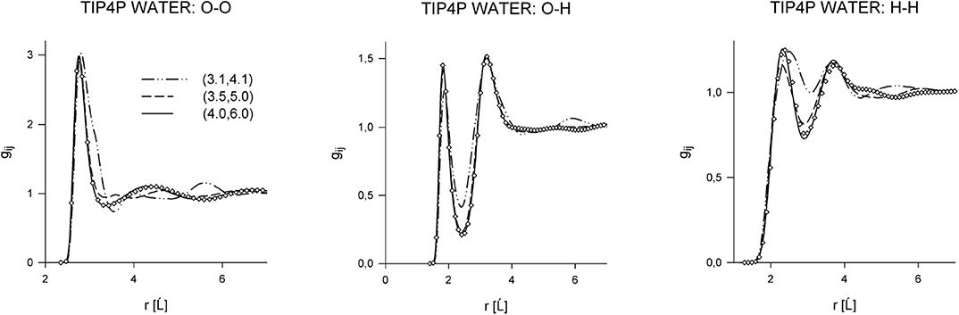
Figure 1. Site-site correlation functions of TIP4P water at ambient conditions in dependence on the switching range, see Equation (25). Curves correspond to different switching ranges, and the circles are simulation results for the full potential.
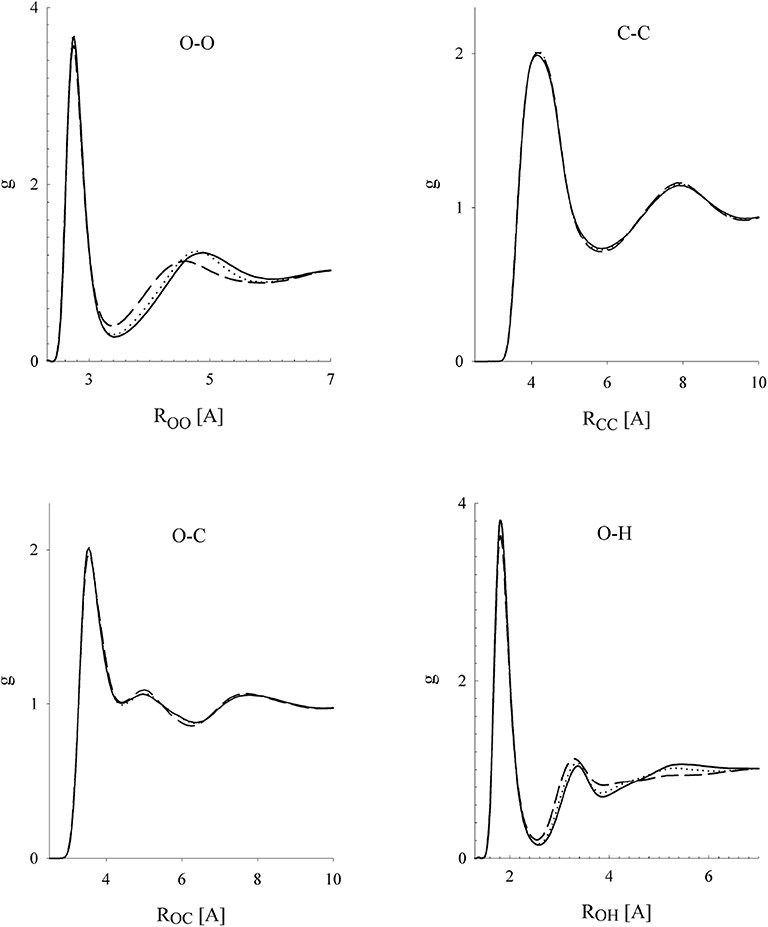
Figure 2. Site-site correlation functions of methanol at density ρ = 761.9 kg/m3 and temperature T = 298 K in dependence on the switching range: dashed line (4,6) [Å]; dotted line (4.7,6.7) [Å]; full line (5.7,7.7) [Å]. Reprinted with permission from J. Phys. Chem. B (2002) 106:7537.
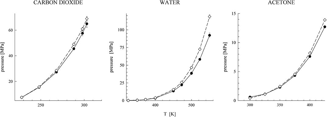
Figure 3. Orthobaric pressures of the full (filled symbols) and short-range versions (open symbols).
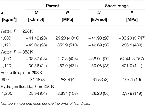
Table 1. Comparison of the internal energy and pressure of the parent and their associated short-range models.
It has therefore been necessary to correct the original interpretation of early simulation results, which has been misleading. The properties of fluids are determined primarily by the short-ranged interactions, which may, however, be not only repulsive (which is the case of simple fluids) but also attractive. In addition to its utilization for equations of state development, this result forms also, for example, the basis for the local molecular field theory of Rodgers et al. [58] who explore a possibility to use a spherical cutoff of the long-range Coulombic interactions. It is also worth mentioning in passing that this conclusion may apply also even to electrolyte solutions as witnessed, for example, by the success of the use of simple short-range models to estimate their properties; see, for example [59–62].
The above findings thus (i) fully justify the use of simple short-range models at all thermodynamic conditions to estimate properties of fluids and (ii) thus explain why equations of state based on simple short-range models (BU approach) may yield reasonably good results. Such models, if properly constructed, should provide an accurate estimate of the structure of both polar and associating fluids but not necessarily of all their thermodynamic properties. In Figure 3, we compare the orthobaric pressure of the full models and their short-range versions for several fluids, and in Table 1 the same comparison is presented for the internal energy and pressure. Whereas the internal energy is also captured quite accurately by the short-range model, this is not the case of pressure, particularly at the dense liquid phase. It means that the contribution of the neglected long-range Coulombic interactions should be the main correction to pressure of the short-range models.
2.5. Primitive Models
We are going to use the term “primitive model” (PM) to refer to simple short-range models (toy models) that capture qualitatively the key physical properties of a given class of fluids but that cannot (should not) be used to estimate quantitatively their thermodynamic properties. For non-polar fluids, the simplest models serving this purpose are purely repulsive hard spheres, various hard bodies, or flexible chains of hard spheres.
To reproduce the structure of polar or associating fluids, the Coulomb interaction at short intermolecular separations has to be incorporated as well. It is assumed that molecules contain charges corresponding to lone electrons and hydrogen atoms (protons). Coulombic-type sites of two kinds (to mimic plus and minus charges and their interaction) are therefore embedded to the hard core of molecules (see Figures 5 and 6). A general primitive model thus assumes the form
where the summation in the second term runs over the pairs of the like sites and in the third term runs over the pairs of the unlike sites. This is a general definition of the primitive model that captures the physical reality, namely that, simultaneously with the attractive interaction between the unlike charges, there is also an inextricable repulsive interaction of the same strength between the like charges. Only these two types of interactions together give rise to H-bonding in real fluids. This corresponds to the TD approach in which the models are not constructed arbitrarily but descend from a realistic parent model. For general rules for the construction of such models see [63, 64]. Two remarks seem here appropriate. First, although the actual choice for the repulsive and attractive site-site interactions seem obvious, a hard sphere interaction for the repulsion and a square-well interaction for the attractive interaction, there are at least two possibilities of defining the attraction between the unlike sites, see Figure 4: (i) Bol [24] defines the attractive interaction between sites i and j with respect to the vector R12 connecting the reference sites
(ii) whereas Smith and Nezbeda [26] defined this interaction directly by the separation between the interaction sites
A consequence of these different definitions is that the orientational part of the configurational space over which an H-bond can be established is constant in Bol's formulation, whereas it is tapered with increasing separation between the reference sites in the SN formulation. Second, the inclusion of the repulsive interaction between the like sites means that when all the attractive interactions are switched off, we do not get a common hard body but the so called pseudohard hard body (PHB) [65], the body that captures the actual excluded volume [66, 67], an important concept in molecular physics of fluids; albeit purely repulsive, it can also yield, to a milder extent, preferred orientations similar to H-bonding [68]. The PHB is not a simple hard body, however; it possesses a flavor of non-additivity, and there is currently no theory for the PHB fluids available.
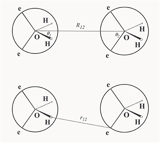
Figure 4. Schematic representation of the H-bonding: Bol's notation (upper) and Smith-Nezbeda's notation (lower).
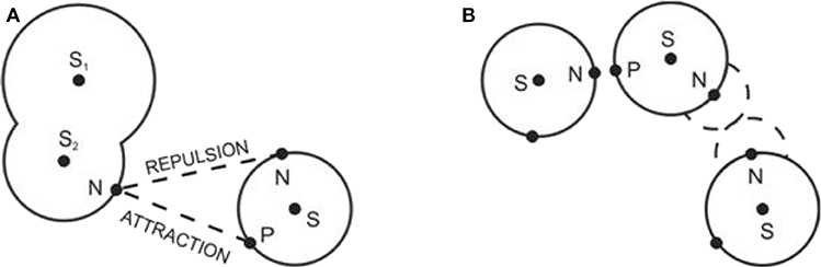
Figure 5. Schematic representation of the site-site interaction in the primitive model (A) and the associated pseudohard body (B). Symbols N and P denote the negatively and positively charged sites, resp. Reprinted with permission from Pure Appl. Chem. (2013) 85:201.
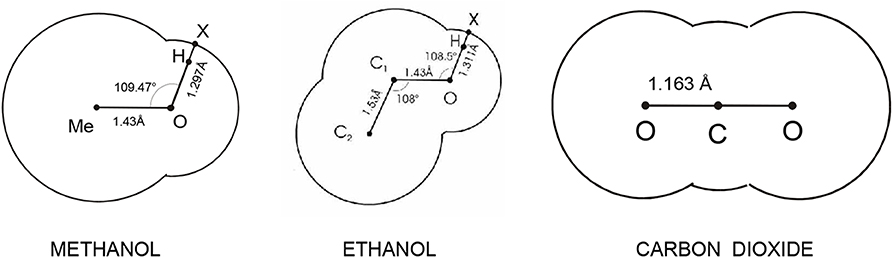
Figure 6. Primitive models descending from realistic force fields.
In general, there are no a priori constraints imposed on model's parameters. Such constraints may be imposed, for example, in connection with the application of a specific theory. For example, to make the application of the TPT possible, it is required that the conditions of the so-called steric incompatibilities be satisfied, see section 2.5.
The above procedures of constructing the primitive models make it possible to examine their structure and, consequently, verify their suitability for the reference fluid. Although the structure is an important physical property, its main use is in theoretical considerations only; in applications with primary focus on the thermodynamic properties, the structure plays only a marginal role. This is the case of the BU approach which focusses on the final net effect of the Coulombic interactions, i.e., on the establishing of H-bonds only, but not on the interactions themselves. It means that in the BU methodology, the second term in (26) is omitted.
Another way for constructing primitive models has thus been followed. Chapman and coworkers, while developing SAFT, utilized the idea of hard bodies with embedded interaction sites and constructed a caricature of molecules also as bodies made up of segments with certain interaction sites [21]. However, bearing in mind the TPT to be used for the evaluation of the thermodynamic behavior of the models, no site location was specified because the TPT of the first order is independent of the site's location. Furthermore, to make the models as simple as possible, and thus (i) easily tractable by theory and (ii) readily applicable to a variety of different fluids, smaller molecules are simply pictured as hard spheres, and larger non-spherical molecules are pictured as chains of hard spheres, see Figure 7. These models (i.e., SAFT models) consequently do not have any relation to real molecules and any realistic intermolecular interaction model, and their actual form is therefore rather arbitrary with all its parameters treated as adjustable.
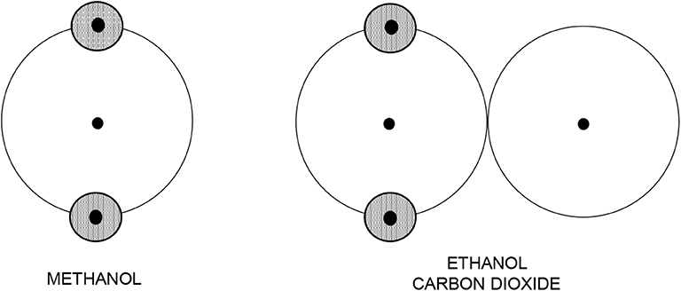
Figure 7. Intuitive primitive models used in SAFT modeling. Shaded circles denote Coulombic interaction sites.
2.6. Thermodynamic Perturbation Theory
The TPT was developed by Wertheim in a series of papers [69–72] to deal with systems exhibiting association or polymerization, i.e., the systems with strongly orientation-dependent and short-ranged attractive interactions with the general interaction in the form of Equation (26). He presented a concise scheme that produces also integral equations (solved analytically, for example, for the one-site SN model [10]). It is not a general theory in the sense that (i) it requires a special form of the interaction function and (ii) explicit results are not universal functions but have to be developed specifically for the model at hand (e.g., number of the interaction sites per molecule). There are two important constraints imposed on the interaction model for the TPT to be applicable, the so-called steric incompatibilities: (1) one interaction site can be engaged in establishing one bond only, and (2) only one bond can be established between two molecules. Provided that these two constraints are not satisfied, the results rapidly start to deteriorate (when compared to simulation data), and when the constraints are ignored, any application of the TPT is only a formal use of certain formulas with unpredictable results. Here we provide only the basic relations of the theory referring the reader to original papers and to a detailed pedagogical review by Zmpitas and Gross [73] for details. For the demonstration of the model dependence and discussion, we present here explicit results for the four-site model, which is a typical model of water (ST2-type models with tetrahedral geometry [74]); explicit expressions of the EoS for different compounds/models can be found in [13] (Equations 22–24 therein).
The TPT theory assumes the interaction function in the form of Equation (26) and starts from its decomposition into a repulsive reference part and a highly directional perturbation part:
where uWref = uhardcore, i.e., the fluid with all attractive interactions switched off, and subscripts “W…” are used to distinguish these potentials from those used in a general perturbation expansion. The quantity addressed by the theory is the excess Helmholtz free energy, AWref, which is expanded about a reference, and, using the diagrammatic technique, it tries to evaluate the contribution due to the association given by uWpert by rearranging the graphs and neglecting certain classes thereof.
The key function of the TPT are integrals I, which involve the Mayer function of the HB bond interaction and (in the first-order theory) the reference (hard body) fluid pair correlation function:
where fHB is the H-bonding Mayer function, fHB = exp(−βuHB) − 1. For a four-site model with two (P)-sites and two (N)-site embedded to a hard sphere, the final result for the residual free energy in the first order expansion is given by [75]
where c is obtained as the solution of a simple equation involving the integral I as a parameter,
As mentioned in the preceding subsection, simple models may have also odd number of Coulombic sites. In this case, one site has to establish two bonds that may cause problems with the application of the TPT—the condition of steric incompatibility is not satisfied. Using the TPT as is in the first order for such models is definitely not correct, but this problem may be bypassed, at least partially, by considering the theory in the second order.
TPT is an approximate theory, and its accuracy is therefore an important issue. Surprisingly, only little attention has been paid to it. Nezbeda et al. [75] examined TPT for a four-site primitive model of water within the context of other theories for primitive models and reported rather disappointing results. A more thorough examination was carried out by Slovak and Nezbeda [76] considering both the site-site and angular interaction formalism. Physical properties examined were the internal energy, pressure (equation of state), and the heat capacity, CP. A general conclusion they drew from the comparison of the theory with the simulation results was that the theory is only fairly accurate at liquid densities and low temperatures and becomes reasonably accurate only at higher temperatures and low densities. They attributed the found discrepancy to only an approximate resummation of graphs at the level of the first order expansion when only one pair of H-bonded molecules is considered in the reference hard body fluid. Better results may be/are obtained from higher order theories. Application of the TPT to water represents a very stringent test. Although no similar examination for simpler models (fluids) has been carried out, it may be assumed that the theory will perform better for other fluids.
Vlček et al. [15] implemented the TPT of the second order and carried out molecular simulations again. Besides a model of water, they also considered a primitive model of methanol that has only one pair of the Coulombic sites. In this latter case, the TPT was in perfect agreement with simulations over the entire range of thermodynamic conditions. The model of water was in perfect agreement with simulations at higher temperatures and at low and intermediate densities; yet the agreement was at least semi-quantitative at very low temperature and high density.
3. Toward an Equation of State
3.1. Perturbed Theoretical Equation of State
As mentioned in section 2.2, to implement the perturbation expansion, a reference fluid has to be determined first, and, according to Equation (13), its correlation function is then required for the correction terms to be evaluated. This step is accomplished by approximating the reference fluid by an appropriate primitive model. In the case of simple fluids, this does not bring about any problem because such a primitive model is the fluid of hard spheres. For other fluids, the primitive model contains both a hard core and an orientation dependent attractive interaction. There are theoretical tools available how to estimate its thermodynamic properties, but this is not the case of correlation functions. Immediately available is the correlation function for the SN model [11], but for other PM models we have to resort to an additional approximation. Integral equations are, with the exception of the Yukawa fluid, out of the question because they yield only numerical results. There thus seems to be only one general tool that may offer an analytic result for g(q1, q2): the RAM (Reference-Average-Mayer function) perturbation theory [77]. Accuracy of this theory was examined by its application to a PM of water [75] with the results found of medium accuracy only. Since it is required that the result be in an analytic form, this would further require additional approximations. Accounting for the fact that the TPT itself may not be sufficiently accurate, it is then questionable whether such an effort is worth trying at all because it is very likely that only a low-quality result can be expected. Nonetheless, the RAM theory can be used for other purposes, see, for example, section 3.3.
It can thus be concluded that there is no theoretical method able to provide a reliable and good description of the structure of the PMs in an analytic form. As it thus stands, it seems that the truly pure theoretical TD approach to develop an analytic EoS has reached its limits.
3.2. van der Waals-Type Approach: SAFT
A typical example of modern vdW-type EoS is the family of SAFT equations. SAFT methodology views molecules as objects built from spherical segments (atoms, molecules, or functional groups) that interact through isotropic interaction forces. It does not consider any explicit intermolecular interaction model but implicitly assumes that there are three major contributions to the total intermolecular interaction energy [22]: (1) the repulsion-attraction contribution between the individual segments (monomers), (2) a contribution due to the formation of chains, and (3) a contribution due to formation of association complex between different segments. The Helmholtz free energy is then written as a sum of three mutually independent contributions, each of them corresponding to the above type of interaction. In terms of the corresponding compressibility factor, it reads as [22]
Decomposition (33) does not have any a priori justification and was based only on intuitive physical considerations in the same way as the original vdW equation. Only later studies on the effect of the range of interactions discussed in section 2.4 have provided a support for it. Specifically, it is the explicit inclusion of the association term because it is the short-range Coulombic interaction, which plays the predominant role. In this respect, Equation (33) should be more appropriately, at least formally, written in another order with zassoc as the leading term.
The monomer-monomer interaction is the subject of choice. The most common choice used to be the LJ potential for which several analytic equations of state are available [2, 78, 79]. The hard-core Yukawa can also be a potential choice for the same reason [47, 48]. It is also used for the description of screed Coulombic interactions while the Sutherland potential is useful for systems with multipolar interactions. The exponents of the LJ potential, (m, n) = (12, 6), were originally chosen for convenience without deeper physical justification. Lafitte et al. [80] let the (m,n) exponents be free adjustable parameters (Mie potential) gaining greater flexibility (two more parameters for fitting) for the description of the softness/hardness of repulsions and also for the range of the attractive interaction. The specific choice of the monomer-monomer interaction also affects the evaluation of the corresponding contribution to the EoS and a lot of effort has also been invested into its development. This activity brings researchers back to the period when perturbation theories of simple fluids were in their focus.
An open question remains whether to directly incorporate also the long-range Coulombic interactions into Equation (33). In their paper [33], Muller and Gubbins conclude that these interactions are more important than it was previously thought and this would also fully agree with the results shown in Table 1. An extension of Equation (33) by including explicitly the dipole-dipole contribution was considered by Karakatsani et al. [81] to deal with strongly dipolar fluids and recently also by Ahem et al. [82]. An extension along the same path was made by Liu et al. [83] who, in addition to incorporating the dipole-dipole interaction, employed the hard-core Yukawa for the monomer-monomer interaction instead of the LJ. On the other hand, Clark et al. [84] argue that this contribution is not necessary and can be captured in an average fashion by short-range primitive models. Although this may be acceptable from the point of final numerical results, this attitude contradicts the primary finding of section 2.4 and takes SAFT farther away from physical reality.
The incorporation of the dipole-dipole interaction contribution to Equation (33) deserves a further discussion. The intermolecular interactions have their origin in the electrostatic interactions whose contribution can be expressed as a sum of multipole-multipole interaction contributions:
This interaction gives rise to the H-bonding phenomenon at short intermolecular separations. It means that it is thus possible to rewrite Equation (34) into the form
where Rcut is a certain cutoff. It becomes now clear that the simultaneous inclusion of the dipole-dipole contribution and the H-bonding contribution means that the dipole-dipole contribution from short intermolecular distances is counted twice: its contribution from the short separations is already accounted for by the H-bonding term. This should be evidently avoided but the question to what extent this double counting affects the results needs to be examined.
To obtain an EoS in an analytic form, the key integrals of type I, Equation (30), have to be evaluated. The integrals contain the correlation function of the reference fluid which, with exception of the fluid of HS, is not available. Since the integration range should be quite narrow, which is required by the conditions of steric incompatibilities, an obvious approximation is to use the rectangular rule for the evaluation of the integral and approximate gHS by its contact value, . Nezbeda and Iglesias-Silva [85] approximated g close to contact by a straight line defined by the contact value of gHS and its first derivative, whereas Jackson et al. [86] used the approximation const. Nonetheless, comparison of simulation results with those based on these approximations showed that the results were nearly identical and that inaccuracies in I had only marginal effect [76]. This finding may thus make evaluation of I easier in cases when the reference fluid is not that of HS because the use of rather crude approximations may be justified.
As is obvious from the above discussion, there is nearly an unlimited number of possibilities to modify or extend SAFT equations. This is in fact the property inherent to any EoS developed using the BU approach and reflects the fact that SAFT is a methodology and not a rigid EoS [22]. It is not the goal of this paper to review SAFT equations, and let us mention therefore at least their main types. Besides the original SAFT with hard sphere monomers, SAFT-HS, two other main versions are SAFT-VR (variable range) [87, 88] and PC-SAFT (perturbed chain) [49]. Furthermore, there is also a group contribution version, SAFT-γ [89], SAFT-RPM [90–92] dealing with electrolytes, and SAFT-VR-D [81, 93] for dipolar and dipolar and associating fluids. The most recent development includes SAFT-μ [80, 94] whose monomer units interact via a Mie-type potential with adjustable exponents. Furthermore, here is a number of modifications and applications of all these versions and we refer the reader to available review articles for further reading [22, 23, 95, 96].
3.3. Equations of State for Water
3.3.1. SAFT Equations
Number of SAFT equations developed for water is enormous. In their recent review from 2016 on SAFT for water, Vega and Llovell [29] list altogether 47 SAFT equations belonging to 9 different versions of SAFT. Yet, many other equations (typically of the same type of equation but with different sets of parameters) are missing. The molecular size and energy parameters of the listed versions vary within the range 1.91–3.59[] for σ and 839–2,932[K] for ϵ/kB pointing again to the fact that these parameters may hardly have anything common with physical reality and are pure numbers. As an interesting example we may mention conclusions of the very recent paper by Ahmed et al. [82]. They report excellent results for the VLE of water and other compounds with one interesting feature: to obtain these results, the size of the monomer unit has to swell with increasing temperature, which contradicts both common sense and the observed (and obtained by theory) behavior; with increasing temperature, the molecules attain kinetic energy and get closer to each other which means that, effectively, their excluded volume shrinks.
The primary question concerns which model of the water molecule to use and all three possibilities, models with two, three, and four Coulombic sites were considered. It is also argued that the number of sites may not be fixed and should be conveniently changed, particularly in aqueous solutions according to solutes. Two-site geometries have therefore also been used. For arguments and discussion of these choices see [29].
There are many papers which include, among other compounds also water but not many papers with the focus on water. An exception are two papers by Jackson et al. [84] and Dufal et al. [94]. The above problem was subject to a thorough research of Clark et al. [84] not from the point of the relation of the water model to reality but which model suits best SAFT. They considered all three possibilities, two, three, and four Coulombic site models. Since the four-site model turned out to yield superior results they furthermore considered four different sets of parameters for this model. They concluded that the model with four Coulombic sites with the W2 set of parameters is the most appropriate in describing the H-bonding in water, yielding the largest ratio of the H-bonding and dispersion energies, and also more realistic degree of association. This could, however, be anticipated, as the four-site arrangement does not give to molecules too many chances to adopt other arrangement but tetrahedral. Despite all the effort invested and careful analysis and discussion in that paper, the recommended parameters are just numbers because the model ignores completely all long-range Coulombic interactions, which is compensated by adjusted values of the parameters.
The other paper [94] discusses in detail an application of the TPT to the model u = uMie + uassoc and it deserves a comment. Although, in general, SAFT assumes some form of the interaction model, we are not aware of any paper where the structure corresponding to the model is examined. The excellent agreement of thermodynamic data may hide deficiencies in the structure which would debase the equation. For example, as a step beyond the hard core with interaction sites, a more “realistic” model, the LJ particle decorated with H-bonding sites was proposed [97]. Nezbeda and Slovak simulated this model [98] with the following result: (i) when the H-bonding energy parameter found in [97] was used, the resulting structure was typically argon-type; (ii) to obtain a water-type structure, it was necessary to increase the energy parameter to a very high value, and the model then behaved like HS with bonding sites. It may be expected that a similar result will be obtained also with the uMie + uassoc model. It would be therefore interesting to examine which structure it will actually produce.
Water is known to exhibit a number of anomalies that seem to be ignored in most applications of SAFT. This is quite surprising because the anomalies are fingerprints of water and their (at least qualitative) reproduction is therefore very important if the equation is to describe the behavior of real water. However, behavior of pure water outside the region of phase equilibria is only rarely addressed. An exception is paper [94] in which some response functions are reported, albeit only at high pressures.
To summarize, there is no doubt that SAFT equations are able to do great job concerning the correlation of experimental data but their contribution to better understanding of the behavior of water has so far been minimal.
3.3.2. Semitheoretical Equations
In their first application of PMs to water, Nezbeda and Pavliček [99] constructed the full EoS similarly as in SAFT fashion with the ST2 geometry of the PM, considering also the dipole-dipole term. The EoS was thus in the form
The dispersion term was considered in its simplest form as the mean field contribution, and the DD term, to avoid double counting of electrostatic contributions at close separation, was assumed as a dipolar hard sphere of a diameter larger than the H-bonding radius. Parameters of the EoS were evaluated, as usual, by fitting the VLE data, and the results were found satisfactory.
A more sophisticated equation along this line was developed by Nezbeda and Weingerl [100] using a four-site parent model and the first-order TPT. The EoS had the same form as above and the parameters were evaluated so as to obtain the best representation of the vapor pressure and coexistence liquid densities from the triple point up to 643.15 K. The equation remains reliable also for various thermodynamic properties outside the coexistence region. It reproduces the anomaly in the isothermal compressibility locating its minimum at T = 38°C (vs. the experimental value T = 46oC) at P = 1 bar. Its overall performance is of the same quality as that of the SAFT-YDD (Yukawa-dipole-dipole) [83] one.
An attempt to derive an equation following the theoretical route was made by Jirsak and Nezbeda [101]. Within the spirit of perturbation theory, we considered modeling water not as a whole but only by its short-range part, and its description by a PM was considered. The parent model was the best non-polarizable model of water, TIP4P/2005 [74]. The short range reference was obtained by deducting its long range Coulombic interaction and the associated PM was then obtained by making use of the RAM [77] and Barker-Henderson theories [6]. The PM thus contained only one parameter, the H-bonding energy ϵ/kB, the parameter which does not exist in the parent model. To keep contact with it (and hence also with real water), they set the value of ϵ/kB to 4440K to obtain, approximately, the experimental temperature of the density maximum and applied the 2nd order TPT developed in [15]. Having in mind that it is the theory of the short-range reference and not of complete water, the qualitative behavior of the response functions, the thermal expansion coefficient, α, the coefficient of isothermal compressibility, κ, and the residual isopiestic heat capacity were examined with the following result. At low pressures, α is a monotonous function that becomes negative with decreasing temperature, which means that the density exhibits a maximum. At elevated pressures, the maximum of ρ moves to lower temperatures in agreement with experimental observations. Another interesting feature of α is crossing of all isobars in a small region around 360 K and α ≈ 0.4 × 10⁻³. This behavior corresponds surprisingly well to that observed on real water: α of real water exhibits the same phenomenon around 325 K with α ≈ 0.45 × 10⁻³. All these findings correspond to rather a very complex behavior of α as a function of pressure along isotherms. The temperature dependence of the coefficient of isothermal compressibility exhibits a minimum that becomes less pronounced with increasing pressure in agreement with the experiment, and there is also a decrease of κ with increasing pressure. The residual isopiestic heat capacity is found to be only weakly temperature dependent, exhibiting, in agreement with reality, a very shallow minimum. The pressure effect on ΔCP is very small.
To summarize, the fact that the proposed theoretical approach reproduces the known anomalies of water semi-quantitatively without any reference to or incorporation of H-bonding should be considered as a great success of theory. Accounting further for the fact that all the results are available in an analytic form this would be the perfect reference system for developing a perturbation-theory-based EoS.
4. Summary and Conclusions
The ultimate goal of the statistical mechanics of matter is to provide methods of explaining and predicting the experimentally measurable quantities of a given substance in terms of the properties of its constituent particles. From the purely theoretical point of view this is feasible because all gears, theories, and simulation methods are readily available. The problem is their implementation. In chemical engineering applications, it is demanded that the obtained equations be in an analytic form while most of the exact statistical mechanical results are in a numerical form only. It is therefore necessary to restore to approximations, but this has to be done with caution. Results of statistical mechanics possess the great power of predictability, whereas too crude approximations may debase them to mere correlation schemes; some recommendations are summarized below.
The theoretical perturbed equations and SAFT equations represent two extreme methods for developing EoS. As already discussed in section 3.1, the theoretical approach is too strictly bound to a parent realistic model which itself has always some deficiency. Furthermore, it also imposes certain limits on theoretical tools, e.g., the simple model used in the process is subject to certain rules. Finally, it may hardly handle fluids made up of large flexible molecules. On the other hand, SAFT is not linked to any real fluid, and its connection with molecular theory is at the same level as it would be the vdW equation in which the original hard sphere term was replaced by the correct EoS of the fluid of HS: a very rough model of molecules is treated by the very sophisticated TPT. Although attempts to improve its performance have been made, these attempts are driven by intuition and analogies only and also keep the resulting EoS only more complex. No doubt that the SAFT equations have been very successful in correlating experimental data, but their potential to predict the properties of fluids in the regions where no data are available—a factor of great importance and necessity—is very questionable.
As it appears, the best way to obtain an accurate and reliable EoS with a potential of predictability may be a combination of both above approaches, i.e., a semi-theoretical approach. It is evident that the crucial point along this way is the choice of a reference fluid that should capture most of the behavior of the studied system (or, more accurately, of the short-range reference fluid) and remove the burden imposed on the correction terms. At this point, the theoretical route may fullfil its role: to supply a primitive model mimicking more or less faithfully real molecules, their interaction, and the structure of the fluid. If this is satisfied, the correction terms will play much less important role and will not need too sophisticated elaboration.
A very important problem is the evaluation of the parameters of equations. It is important to bear in mind that the primitive model should reproduce as faithfully as possible the properties of the reference fluid and not of the considered fluid. It means that the parameters of the primitive model and of the correction terms have to be evaluated separately, which will make this route different from the current SAFT and previous semitheoretical approaches. Concerning the evaluation of the parameters of the correction terms, this is discussed in [84]. A typical choice used in the majority of papers on SAFT are vapor-liquid equilibrium (VLE) data. Clark et al. discuss this problem and are aware of the fact that the pairwise additive force fields are not able, in principle, to describe simultaneously the behavior of liquid and gas [102] of strongly associating fluids and that only the orthobaric pressures and liquid saturated densities should be used in fitting.
Another important problem concerns the inclusion of the dipole-dipole interaction. The best and simplest, and also most commonly used, is the Padé approximant of Rushbrook et al. [103]. However, its incorporation is not straightforward, which is not always recognized. It is not possible to formally add this term as is to the EoS. As mentioned in section 3.2, the dipole-dipole interaction at short separations is part of the electrostatic interactions that result in H-bonding and is thus already included in the models with the explicit H-bonding terms. If this is not taken care of, the electrostatic interaction at short separations will be counted twice. To assess the importance/effect of this inconsistency remains to be done.
An associated problem is the choice of properties to use to assess the developed EoS. In the overwhelming majority cases, how accurately the equation can correlate the equilibrium data is reported as a rule despite the fact that such data were, at least partially, used for the evaluation of the parameters. It is not necessary to bother with the structure because this should be the problem of the primitive model to be developed. We think that the useful and fair way to assess accuracy/correctness of the EoS is to go away from the phase equilibrium region and to present the response functions, i.e., the second derivatives of the Helmholtz free energy. Not only water but also other associating fluids exhibit an interesting behavior of these functions. This comparison could cast light on the quality of the derived equation.
The last remark concerns the future development. In this review, we have focused on pure fluids, which is of importance for theory, but in applications, we have to deal primarily with mixtures. Mixtures were in the focus of research in the early stages of the development of theories of fluids, but we are not aware of any systematic theoretical research activities at the present time. Moreover, whereas for pure fluids force fields are being continuously developed and improved, practically no results are available for the intermolecular interaction between the molecules of species A and B. In other words, the effect of the presence of molecule B on the pair interaction A–A is not known, and empirical combining rules must be employed. This deficiency could be, at least partially, bypassed by employing polarizable force fields but then the theoretical path is out of question. Consequently, a SAFT-type approach remains at present the only available tool to deal with mixtures (and other complex problems such as for example, interfacial phenomena). With regards to theory, it can be assumed that the effect of the range of interactions found for pure liquids will hold true also for mixtures. A natural choice for the reference system will then be a mixture of primitive models, though with the only exception [104] that results for the thermodynamic properties of such mixtures are missing. It is generally accepted that excluded volume effects are responsible for a number of observed properties of mixtures, and the primitive models (or their pseudohard cores) may capture them. It is also known that mixtures/solutions, e. g., aqueous solutions of alcohols, exhibit anomalies in their structural properties and primitive models may be able to capture them. All these theoretical results may lead to a more sophisticated reference system, which is the key to developing accurate and reliable equations of state.
Author Contributions
The author confirms being the sole contributor of this work and has approved it for publication.
Funding
Support for this work was provided by the Czech Science Foundation (Grant No. 20-06825S).
Conflict of Interest
The author declares that the research was conducted in the absence of any commercial or financial relationships that could be construed as a potential conflict of interest.
References
1. Wagner W, Pruss, A. The IAPWS formulation 1995 for the thermodynamic properties of ordinary water substance for general and scientific use. J Phys Chem Ref Data. (2002) 31:387–535. doi: 10.1063/1.1461829
2. Johnson JK, Zollweg JA, Gubbins KE. The Lennard-Jones equation of state revisited. Mol Phys. (1993) 78:591–618.
4. Nezbeda I. Analytic solution of Percus-Yevick equation for fluid of hard spheres. Czech J Phys B. (1974) 24:55–62.
5. Jelinek J, Nezbeda I. Analytic solution of the Percus-Yevick equation for sticky hard sphere potential. Phys A. (1976) 84:175–87.
6. Barker JA, Henderson D. What is “liquid”? Understanding the states of matter. Rev Mod Phys. (1976) 48:587–671.
7. Nezbeda I. Percus-Yevick theory for the system of hard spheres with a square-well attraction. Czech J Phys. (1977) 27:247–54.
8. Wertheim MS. Exact solution of mean spherical model for fluids of hard spheres with permanent electric dipole moments. J Chem Phys. (1971) 55:4291–8.
9. Dahl LW, Andersen HC. A theory of the anomalous thermodynamic properties of liquid water. J Chem Phys. (1983) 78:1980–93.
10. Wertheim MS. Integral-equation for the Smith-Nezbeda model of associated fluids. J Chem Phys. (1988) 88:1145–55.
11. Kalyuzhnyi YV, Nezbeda I. Analytic solution of the Wertheim's OZ equation for the Smith-Nezbeda model of associated liquids. Mol Phys. (1991) 73:703–13.
12. Kolafa J, Nezbeda I. Implementation of the Dahl-Andersen-Wertheim theory for realistic water-water potentials. Mol Phys. (1989) 66:87–95.
13. Kolafa J, Nezbeda I. Primitive models of associated liquids: equation of state, liquid-gas phase transition and percolation threshold. Mol Phys. (1991) 72:777–85.
14. Slovak J, Nezbeda I. Extended 5-site primitive models of water: theory and computer simulations. Mol Phys. (1997) 91:1125–36.
15. Vlcek L, Slovak J, Nezbeda I. Thermodynamic perturbation theory of the second-order: implementation for models with double-bonded sites. Mol Phys. (2003) 101:2921–7. doi: 10.1080/00268970310001606795
16. Tang Y, Tong Z, Lu B. Analytic equation of state based on the Ornstein-Zernike equation. Fluid Phase Equil. (1997) 134:21–42.
17. Reiner A, Hoye JS. Self-consistent Ornstein-Zernike approximation for the Yukawa fluid with improved direct correlation function. J Chem Phys. (2008) 128:114507. doi: 10.1063/1.2894474
18. Heinen M, Holmquist P, Banchio AJ, Nagele G. Pair structure of the hard-sphere Yukawa fluid: an improved analytic method versus simulations, Rogers-Young scheme, and experiment. J Chem Phys. (2011) 134:044532. doi: 10.1063/1.3524309
19. Sun JX. Analytical equations of state for multi-Yukawa fluids based on the Ross variational perturbation theory and the Percus-Yevick radial distribution function of hard spheres. Mol Phys. (2007) 105:3139–44. doi: 10.1080/00268970701769938
20. Chapman WG, Gubbins KE, Jackson G, Radosz M. SAFT - equation-of-state solution model for associating fluids. Fluid Phase Equil. (1989) 52:31–8.
21. Chapman WG, Gubbins KE, Jackson G, Radosz M. New reference equation of state for associating liquids. Ind Eng Chem Res. (1990) 29:1709–21.
22. Muller EA, Gubbins KE. Molecular-based equations of state for associating fluids: a review of SAFT and related approaches. Ind Eng Chem Res. (2001) 40:2193–211. doi: 10.1021/ie000773w
23. McCabe C, Galindo A. SAFT associating fluids and fluid mixtures. in eds Goodwin ARH, Sengers JV, Peters CJR, editors. Applied Thermodynamics of Fluids. The Royal Society of Chemistry (2010). p. 215–79.
24. BoL W. Monte-Carlo simulations of fluid systems of waterlike molecules Mol Phys. (1982) 45:605–16.
25. Dahl LW, Andersen HC. cluster expansions for hydrogen-bonded fluids. 3. Water J Chem Phys. (1983) 78:1962–79.
27. Huang SH, Radosz M. Equation of state for small, large, polydisperse, and associating molecules. Ind Eng Chem Res. (1990) 29:2284–94.
28. Huang SH, Radosz M. Equation of state for small, large, polydisperse, and associating molecules - extension to fluid mixtures. Ind Eng Chem Res. (1991) 30:1994–2005.
29. Vega LF, Llovall F. Review and new insights into the application of molecular-based equations of state to water and aqueous solutions. Fluid Phase Equil. (2016) 416:150–73. doi: 10.1016/j.fluid.2016.01.024
31. Boublik T, Nezbeda I. P-V-T behaviour of hard body fluids. Theory and experiment. Coll Czech Chem Commun. (1986) 51:2301–432.
32. Gray CG, Gubbins KE, Joslin CG. Theory of Molecular Fluids. Vol. 2. Oxford: Oxford Univ. Press (2011).
33. Muller EA, Gubbins K. An equation of state for water from a simplified intermolecular potential. Ind Chem Eng Res. (1995) 34:3662–73.
34. Nezbeda I. On molecular-based equations of state: rigor versus speculations. Fluid Phase Equil. (2001) 182:3–15. doi: 10.1016/S0378-3812(01)00375-2
36. Chapman WG, Gubbins KE, Joslin CG, Gray CG. Theory and simulation of associating liquid-mixtures. Fluid Phase Equil. (1986) 29:337–46.
37. Kolafa J, Nezbeda I. Monte Carlo simulations on primitive models of water and methanol. Mol Phys. (1987) 61:161–75.
38. Nezbeda I. Simple short-ranged models of water and their application. A review. J Mol Liq. (1997) 73–4:317–36.
39. Vlcek L., Nezbeda I. Thermodynamics of simple models of associating fluids: primitive models of ammonia, methanol, ethanol, and water. Mol Phys. (2004) 102:771–81. doi: 10.1080/00268970410001705343
40. Vlcek L, Nezbeda I. From realistic to simple models of fluids. III. Primitive models of carbon dioxide, hydrogen sulphide, and acetone, and their properties. Mol Phys. (2005) 103:1905–15. doi: 10.1080/00268970500083630
41. Sciortino F. Primitive models of patchy colloidal particles. A review. Coll Czech Chem Commun. (2010) 75:349–58. doi: 10.1135/cccc2009109
42. Bianchi E, Blaak R, Likos CN. Patchy colloids: state of the art and perspectives Phys Chem Chem Phys. (2011) 13:6397–410. doi: 10.1039/c0cp02296a
43. Boublik T, Nezbeda I, Hlavaty K. Statistical Thermodynamics of Simple Liquids and Their Mixtures. Amsterdam: Elsevier (1980).
46. Nezbeda I, Smith WR. The use of a site-centered coordinate system in the statistical mechanics of site interaction molecular fluids. Chem Phys Lett. (1981) 81:79–82.
47. Duh DM, Mier-Y-Teran L. An analytical equation of state for the hard-core Yukawa fluid. Mol Phys. (1997) 90:373–80.
48. Montes J, Robles M, Lopez de Haro M. Equation of state and critical point behavior of hard-core double-Yukawa fluids J Chem Phys. (2016) 144:084503. doi: 10.1063/1.4942199
49. Gross J, Sadowski G. Perturbed-chain SAFT: an equation of state based on a perturbation theory for chain molecules. Ind Eng Chem Res. (2001) 40:1244–60. doi: 10.1021/ie0003887
50. Nezbeda I. Towards a unified view of fluids. Mol Phys. (2005) 103:59–76. doi: 10.1080/0026897042000274775
51. Nezbeda I. Structure of water: short-ranged versus long-ranged forces. Czech J Phys B. (1998) 48:117–22.
52. Nezbeda I, Kolafa J. Effect of short- and long-range forces on the structure of water: temperature and density dependence. Mol Phys. (1999) 97:1105–16.
53. Kolafa J, Nezbeda I. Effect of short- and long-range forces on the structure of water. II. Orientational ordering and the dielectric constant. Mol Phys. (2000) 98:1505–20. doi: 10.1080/00268970009483356
54. Kolafa J, Nezbeda I, Lisal M. Effect of short- and long-range forces on the properties of fluids. III. Dipolar and quadrupolar fluids. Mol Phys. (2001) 99:1751–64. doi: 10.1080/00268970110072386
55. Kettler M, Nezbeda I, Chialvo AA, Cummings PT. Effect of the range of interactions on the properties of fluids. Phase equilibria in pure carbon dioxide, acetone, methanol, and water. J Phys Chem B. (2002) 106:7537–46. doi: 10.1021/jp020139r
56. Chialvo AA, Kettler M, Nezbeda I. Effect of the range of interactions on the properties of fluids. Part II. Structure and phase behavior of acetonitrile, hydrogen fluoride, and formic acid. J Phys Chem B. (2005) 109:9736–50. doi: 10.1021/jp050922u
57. Zhou S, Solana JR. Progress in the perturbation approach in fluid and fluid-related theories. Chem Res. (2009) 109:2829–58. doi: 10.1021/cr900094p
58. Rodgers JM, Hu Z, Weeks JD. On the efficient and accurate shirt-range simulations of uniform polar molecular fluids. Mol Phys. (2011) 109:1195–211. doi: 10.1080/00268976.2011.554332
59. Nezbeda I. Can we understand (and model) aqueous solutions without any electrostatic interactions? Mol Phys. (2001) 99:1631–9. doi: 10.1080/00268970110064781
60. Nezbeda I. Modeling of aqueous electrolytes at a molecular level: Simple short-range models and structure breaking and structure enhancement phenomena. J Mol Liquids (2003) 103-4C:309–17. doi: 10.1016/S0167-7322(02)00149-6
61. DeMille RC, Molinero V. Coarse-grained ions without charges: Reproducing the solvation structure of NaCl in water using short-ranged potentials. J Chem Phys. (2009) 131:034107. doi: 10.1063/1.3170982
62. Drunsel F, Gross J. Theory of model electrolyte solutions: Assessing the short- and long-ranged contributions by molecular simulations. Fluid Phase Equil. (2016) 430:195–206. doi: 10.1016/j.fluid.2016.09.026
63. Nezbeda I, Vlcek L. Thermophysical properties of fluids: From realistic to simple models and their applications. Int J Thermophys. (2004) 25:1037–49. doi: 10.1023/B:IJOT.0000038498.47700.3f
64. Vlcek L, Nezbeda I. From realistic to simple models of associating fluids. II. Primitive models of ammonia, ethanol, and models of water revisited. Mol Phys. (2004) 102:485–97. doi: 10.1080/00268970410001668417
66. Nezbeda I, Rouha M. Extended excluded volume: its origin and consequences. Pure Appl Chem. (2013) 85:201–10. doi: 10.1351/PAC-CON-12-04-04
67. Rouha M, Nezbeda I. Excess properties of aqueous solutions: Hard spheres versus pseudo-hard bodies. Mol Phys. (2011) 109:613–7. doi: 10.1080/00268976.2010.542779
68. Nezbeda I, Skvor J. Excluded volume versus hydrogen bonding: complementary or incompatible concepts? Mol Phys. (2012) 110:2987–92. doi: 10.1080/00268976.2012.689875
69. Wertheim MS. Fluids with highly directional attractive forces: I. Statistical thermodynamics. J Stat Phys. (1984) 35:19–34.
70. Wertheim MS. Fluids with highly directional attractive forces: II. Thermodynamic perturbation theory and integral equations. J Stat Phys. (1984) 35:35–47.
71. Wertheim MS. Fluids with highly directional attractive forces: III. Multiple attraction sites. J Stat Phys. (1986) 42:459–76.
72. Wertheim MS. Fluids with highly directional attractive forces: IV. Equilibrium polymerization. J Stat Phys. (1986) 42:477–92.
73. Zmpitas W, Gross J. Detailed pedagogical review and analysis of Wertheim's thermodynamic perturbation theory. Fluid Phase Equil. (2016) 428:121–52. doi: 10.1016/j.fluid.2016.07.033
74. Vega C, Abascal JLF. Simulating water with rigid non-polarizable models: a general perspective. Phys Chem Chem Phys. (2011) 13:19663–88. doi: 10.1039/c1cp22168j
75. Nezbeda I, Kolafa J, Kalyuzhnyi YV. Primitive model of water. II. Theoretical results for the structure and thermodynamic properties. Mol Phys. (1989) 68:143–60.
76. Slovak J, Nezbeda I. On accuracy of Wertheim's thermodynamic perturbation theory for primitive models of water. Mol Phys. (2003) 101:789–98. doi: 10.1080/0026897031000075633
77. Smith WR, Nezbeda I, Melnyk TW, Fitts DD. Reference system selection and the average Mayer-function perturbation theory for molecular fluids. Faraday Discuss Chem Soc. (1978) 66:130–7.
78. Kolafa J, Nezbeda I. The Lennard-Jones fluid: an accurate analytic and theoretically-based equation of state. Fluid Phase Equil. (1994) 100:1–34.
79. Thol M, Rutkai G, Koster A, Lustig R, Span R, Vrabec J. Equation of state for the Lennard-Jones fluid. J Phys Chem Ref Data. (2016) 45:023101. doi: 10.1063/1.4945000
80. Lafitte T, Apostolakou A, Avenda C, Galindo A, Adjiman CS, Muller EA, et al. Accurate statistical associating fluid theory for chain molecules formed from Mie segments. J Chem Phys. (2013) 139:154504. doi: 10.1063/1.4819786
81. Karakatsani EK, Spyriouni T, Economou IG. Extended Statistical Associating FLuid Theory (SAFT) equations of state for dipolar fluids. AIChE J. (2005) 51:2328–42. doi: 10.1002/aic.10473
82. Ahmed S, Ferrando N, de Hemptinne JC, Simonin JP, Bernard O, Baudouin O. A new PC-SAFT model for pure water, water-hydrocarbons, and water-oxygenates systems and subsequent modeling of VLE, VLLE, and LLE. J Chem Eng Data. (2016) 61:4178–90. doi: 10.1021/acs.jced.6b00565
83. Liu ZP, Li YG, Chan KY. Equation of state for nonpolar, polar, chain, and associating fluids based on the dipolar Yukawa potential. Ind Eng Chem Res. (2001) 40:973–79. doi: 10.1021/ie000627q
84. Clark GNI, Haslam AJ, Galindo A, Jackson G. Developing optimal Wertheim-type models of water for use in Statistical Association Fluid Theory (SAFT) and related approaches. Mol Phys. (2006) 104:3561–81. doi: 10.1080/00268970601081475
85. Nezbeda I, Iglesias-Silva GA. Primitive model of water. III. Analytic theoretical results with anomalies for the thermodynamic properties. Mol Phys. (1990) 69:767–74.
87. Gil-Villegas A, Galindo A, Whitehead PJ, Mills SJ, Jackson G, Burgess AN. Statistical associating fluid theory for chain molecules with attractive potentials of variable range. J Chem Phys. (1997) 106:4168–86.
88. Patel BH, Docherty H, Varga S, Galindo A, Maitland GC. Generalized equation of state for square-well potentials of variable range? Mol Phys. (2005) 103:129–39. doi: 10.1080/00268970412331303990
89. Lymperiadis A, Adjiman CS, Galindo A, Jackson G. A group contribution method for associating chain molecules based on the statistical associating fluid theory (SAFT-gamma). J Chem Phys. (2007) 127:234903. doi: 10.1063/1.2813894
90. Tan SP, Ji X, Adidharma H, Radosz M. Statistical associating fluid theory coupled with restrictive primitive model extended to bivalent ions. SAFT2: 1. Single salt plus water solutions. J Phys Chem B. (2006) 110:16694. doi: 10.1021/jp0625107
91. Tan SP, Ji X, Adidharma H, Radosz M. Statistical associating fluid theory coupled with restrictive primitive model extended to bivalent ions. SAFT2: 2. Brine/seawater properties predicted. J Phys Chem B. (2006) 110:16700. doi: 10.1021/jp062511z
92. Eriksena DK, Lazarou G, Galindo A, Jackson G, Adjiman CS, Haslam AJ. Development of intermolecular potential models for electrolyte solutions using an electrolyte SAFT-VR Mie equation of state. Mol Phys. (2016) 114:2724–9. doi: 10.1080/00268976.2016.1236221
93. dos Ramos MC, Goff KD, Zhao H, McCabe C. Modeling the phase behavior of H2S+n-alkane binary mixtures using the SAFT-VR+D approach. J Phys Chem B. (2008) 112:9417–27. doi: 10.1021/jp800397n
94. Dufal S, Lafitte T, Haslam A, Galindo A, Clark GNI, Vega C, et al. The A in SAFT: developing the contribution of association to the Helmholtz free energy within a Wertheim TPT1 treatment of generic Mie fluids. Mol Phys. (2015) 113:948–84. doi: 10.1080/00268976.2015.1029027
95. Economou IG. Statistical associating fluid theory: a successful model for the calculation of thermodynamic and phase equilibrium properties of complex fluid mixtures. Ind Eng Chem Res. (2002) 41:953–62. doi: 10.1021/ie0102201
96. Tan SP, Adidharma H, Radosz M. Recent advances and applications of statistical associating fluid theory. Ind Eng Chem Res. (2008) 47:8063–82. doi: 10.1021/ie8008764
97. Chapman WG. Prediction of the thermodynamic properties of associating Lennard-Jones fluids - theory and simulation. J Chem Phys. (1990) 93:4299–304.
98. Nezbeda I, Slovak J. Can Lennard-Jones particles with four bonding sites realistically model water? Chem Phys Lett. (1996) 260:336–40.
99. Pavlicek J, Nezbeda I. Application of primitive models of association: a simple theoretical equation of state of water. Fluid Phase Equil. (1996) 116:530–6.
100. Nezbeda I, Weingerl U. A molecular-based theory for the thermodynamic properties of water. Mol Phys. (2001) 99:1595–606. doi: 10.1080/00268970110064790
101. Jirsak J, Nezbeda I. Towards a statistical mechanical theory of water: analytical theory for a short-ranged reference system. J Chem Phys. (2007) 127:12450. doi: 10.1063/1.2771547
102. Rouha M, Nezbeda I, Hruby J, Moucka F. Higher virial coefficients of water. J Mol Liq. (2018) 270:81–6. doi: 10.1016/j.molliq.2017.11.105
103. Rushbrook GS, Stell G, Hoye JS. Theory of polar liquids I. Dipolar hard spheres Mol Phys. (1973) 26:1199–215.
Keywords: perturbation theory, simple reference fluids, classification of equations of state, primitive models, thermodynamic perturbation theory, SAFT equations
Citation: Nezbeda I (2020) On Molecular-Based Equations of State: Perturbation Theories, Simple Models, and SAFT Modeling. Front. Phys. 8:287. doi: 10.3389/fphy.2020.00287
Received: 10 April 2020; Accepted: 25 June 2020;
Published: 29 September 2020.
Edited by:
Susana Figueroa-Gerstenmaier, University of Guanajuato, MexicoReviewed by:
Ana Laura Benavides, University of Guanajuato, MexicoVíctor Manuel Trejos Montoya, Autonomous University of the State of Hidalgo, Mexico
Copyright © 2020 Nezbeda. This is an open-access article distributed under the terms of the Creative Commons Attribution License (CC BY). The use, distribution or reproduction in other forums is permitted, provided the original author(s) and the copyright owner(s) are credited and that the original publication in this journal is cited, in accordance with accepted academic practice. No use, distribution or reproduction is permitted which does not comply with these terms.
*Correspondence: Ivo Nezbeda, ivonez@icpf.cas.cz