


Abstract
The neutral ionisation model proposed by Groebner et al (2002 Phys. Plasmas9 2134) to determine the plasma density profile in the H-mode pedestal, is extended to include charge exchange processes in the pedestal stimulated by the ideas of Mahdavi et al (2003 Phys. Plasmas10 3984). The model is then tested against JET H-mode pedestal data, both in a 'standalone' version using experimental temperature profiles and also by incorporating it in the Europed version of EPED. The model is able to predict the density pedestal over a wide range of conditions with good accuracy. It is also able to predict the experimentally observed isotope effect on the density pedestal that eludes simpler neutral ionization models.
Export citation and abstract BibTeX RIS

Original content from this work may be used under the terms of the Creative Commons Attribution 4.0 license. Any further distribution of this work must maintain attribution to the author(s) and the title of the work, journal citation and DOI.
1. Introduction
Core energy confinement in tokamaks operating in H-mode is sensitive to the properties of the associated edge pedestal. Specifically, the limiting core temperature profile is believed to be 'stiff', i.e. determined by marginal stability to ion temperature gradient modes [1]. Consequently, it is largely controlled by the boundary condition on the temperature at the top of the H-mode temperature pedestal. Thus, a reliable model for this pedestal is a key requirement for predicting the performance of burning plasma designs, such as ITER or the proposed spherical tokamak STEP.
The EPED model [2] based on the requirement that the pedestal plasma pressure profile is stable to both kinetic ballooning modes (KBMs) and peeling-ballooning modes [3] is often invoked for this purpose. The former is used to set the pressure gradient and the latter to provide the width of the pedestal, together yielding the pressure at the pedestal top. However, one really needs individual models for the profiles of the pedestal ion and electron temperatures,  and
and  , respectively, and the plasma density profiles,
  . There is support from JET for a model for the electron temperature profile in the pedestal based on transport due to electron temperature gradient (ETG) turbulence [4] but this depends strongly on the profile of the parameter
  : hence one also needs a prescription for the electron density profile to complete this model. This has usually been taken as an experimental input, but some success has been obtained with a theoretically based transport model invoking the source provided by ionisation of neutral particles incident from the scrape-off layer (SOL), together with a pedestal diffusion coefficient,
  [5, 6]. This could be related to the same ETG turbulence [7] and/or to KBMs and the neoclassical (NC) transport [8].
The neutral ionisation model described in [5], which considers the ionisation of the incident low energy, Franck–Condon neutrals produced by recycling and gas-puffing incident at the separatrix, has been tested against experimental data from DIII-D [5], MAST [9] and JET [10]. The enhanced version presented in [6] includes the effects of the incident higher energy, charge-exchange population generated in the SOL which penetrate further into the plasma column. In this work we use similar ideas to provide a simple model for the effect of charge-exchange processes in the pedestal region.
The ionisation model is described in section 2, while in section 3 we describe two implementations of the model for testing against the JET data. First it is used with experimental temperature profiles, which we refer to as the 'standalone' version. Then the ionisation model is introduced into the EPED model in the Europed code where both the density and temperature pedestals are predicted self-consistently. In section 4 we investigate the sensitivity of the model to its parameters. Section 5 investigates the predictions of the model regarding the isotope effect. Section 6 provides a summary and discussion with some conclusions.
2. The ionisation model for the density profile
2.1. Transport equations
In the spirit of [6], which develops the model in [5] further, we obtain the radial profile of the electron density,  in the H-mode pedestal region by balancing radial diffusion, with coefficient
  against ionisation by both low energy Franck–Condon and more energetic charge exchange neutrals, with densities
  and
and  , respectively, themselves being modelled by balancing inward convection against ionisation and charge exchange sources and sinks.
We use straight field line coordinates:  , with Jacobian
  , where
  is the major radius, its value on the magnetic axis being
  , the 'minor radius' co-ordinate
  is a flux surface label and
  are poloidal and toroidal angles, respectively. In the narrow pedestal region, we introduce the radial co-ordinate,
  , where
  is the radius of the separatrix flux surface,
  .
.
The ionisation model described above is represented by the three equations:


Introducing the straight field line co-ordinates and averaging over the poloidal angle 
where  and
and  are the ionisation and charge exchange rates, respectively, while
  and
and  are the corresponding radial velocities of the two species, each considered to be mono-energetic. Thus,
  ,
,  , where
  are the corresponding cross-sections, which will vary with electron and ion temperatures, and
  and
and  are the electron and ion thermal speeds respectively. For the radial velocities of the neutrals, we follow [6], setting
  , with
  and
and  (we drop the suffix
  , below). The factor ½ in equation (3) represents the fact that the outward flux of fast charge exchange neutrals is taken to be lost. The diffusion coefficient
  may have a profile dependence arising from dependencies on
  and
and  . In the modelling described later, we suppose it arises from a combination of ETG and KBM turbulence and NC transport.
A similar set of equations were proposed in the SOL in [6], while those in [5] follow on neglecting  .
.
It is convenient to introduce a flux surface average over poloidal angle:  . To make the system of equations (4)–(6) readily tractable we introduce two form factors:

If the source of the Franck Condon neutrals is localised, say at some angle  , then
  , whereas the charge exchange scattering may produce a more isotropic distribution of charge exchange neutrals with
  tending to unity. In general, one needs a numerical simulation of the neutral processes to evaluate these quantities precisely; alternatively, they could be treated as fitting parameters.
2.2. Solution procedure
Using the expressions (7), equation (5) implies

while combining this result with equation (6) yields
Inserting these two results into equation (4) and integrating once, we obtain
Here  is a constant of integration that is determined by the condition that deep into the plasma, both neutral densities should vanish. It is to be remarked that in [5],
  was arbitrarily set to zero, whereas we now allow the more realistic finite density gradient inboard of the pedestal.
Equations (4) and (10) provide an expression for  in terms of
  :
:
and then  follows from equation (9). The electron density profile is then given by the third order equation

where the non-linear, second order operator  is defined by:

It may be more convenient to replace this third order equation by an iterative solution based on a second order equation. Using equation (10) to replace  and introducing the solution of equation (8) for
  yielding
Equation (4) becomes

The integral in the last term can be iterated in  until one has a self-consistent solution of equation (15) for
  A convenient starting point is the solution of equation (4) in the absence of
  . In this limit, equation (4) reduces to
The presence of  prevents obtaining the analytic solution obtained in [5], so this equation must be solved numerically before inserting its solution in equation (15) to begin the iterative process.
However, the form of equation (15) obscures how it reduces to the equation derived in [5] when charge exchange neutrals are omitted from the model. This limit is evident if one derives the second order equation for  involving
  , rather than
  as in equation (15):

Here the charge exchange neutral density,  , is given in terms of
  by the solution of equation (9):
2.3. Boundary conditions
The original set of equations (1)–(3) form a fourth order system requiring four boundary-conditions. Correspondingly, the third-order equation (12) naturally requires three boundary-conditions, to be added to that following from the constant of integration,  , i.e.,
  . Thus, the separatrix values of the electron density,
  , its radial gradient,
  and the Franck–Condon neutrals,
  would suffice. Alternatively, one could use equation (11) to replace
  by
by  , so that all boundary conditions could be expressed in terms of
  . However, it is more appropriate to remain with the specification of
  or, equivalently, the incident flux at the separatrix of such neutrals:
  It is of interest that the charge exchange density, and hence
  specifically, follows directly from equation (10).
Mahdavi et al [6] proposed a simple model for the neutral interactions in the SOL to provide the ratio  , rather than considering this as an input to the boundary conditions. Furthermore, by considering the SOL region one can also determine
  . Thus, the source-free solution for the electron density, where radial diffusion with a diffusion coefficient
  is balanced by streaming along the open magnetic field lines on a timescale
  , follows from the equation
namely  . Thus

3. Model results for the JET pedestal database
The JET database [11] with more than 1000 fitted pedestal profiles of JET plasmas is used to test the model. For the model, we can obtain the boundary conditions  and
and  from the experimental data.
  is assumed to be known as well for a given device. We set
  to a value of 1015 m−3 and
  = 0.001 s but note that the results are to some extent sensitive to these values. Since we have no good reduced model for the poloidal distribution of the neutrals, we set both
  and
and  to 1, that assumes equal distribution with the poloidal angle. Thus,
  is the only free parameter to be modelled. In this work we have implemented the model described in [7], where
  is constructed from three components, the first driven by ETG turbulence is proportional to the electron heat transport, the second from NC transport and the third driven by KBMs is proportional to the extent to which the normalized pressure gradient (
 ) exceeds the threshold value for KBMs. The ETG part can be calculated from the known heat flux through pedestal and the temperature profile using the normal heat conduction equation:

where  is the heat flux at the pedestal as calculated from the input heating power and the plasma geometry,
  , where
  is the total heating power to electrons (assumed for simplicity to be half of the total power throughout the modelling) and S is the surface area of the plasma. The particle transport from ETG is set to be this multiplied by a constant factor
  and so

We keep the value of  open at this point and recognize that even if we label it as 'ETG' it covers all the mechanisms that are responsible of the heat transport through the pedestal region (including other turbulent transport and ELMs), i.e. it only excludes NC and KBM transport.
Following [7], the NC part of  is taken for simplicity to be

Finally, again following [7], the KBM part of diffusion coefficient  is assumed to be zero below the KBM stability limit and then increase proportionally to
  , where
  is the normalised pressure gradient in the pedestal defined [12] as
Here  is the volume enclosed by the flux surface,
  is the major radius,
  is the pressure and the derivative, represented by
  , is taken with respect to the poloidal flux
  and
and  is the stability limit of the KBMs. Since KBMs have a wide radial extent [8], we assume that the particle transport from them is not local but covers the entire pedestal region. Therefore, instead of a local value of
  , we use the average value in the pedestal region. The total
  from KBM is given by the formula:
The combined particle diffusion coefficient is then

with  and
and  as adjustable parameters. We also assume that the radial particle diffusion outside the separatrix matches that with the particle diffusion inside the separatrix, i.e. we assume that
  in equation (20) is the same as the value of
  at the separatrix.
3.1. Standalone model using the experimental temperature profiles
With the assumptions above, we simulated the entire JET-ILW database using the experimental temperature profile to calculate the ionisation and charge exchange cross-sections,  and
and  [13],
[13],  , needed in equation (22), and
  needed in equation (25) (
 is calculating by scaling the value in a known equilibrium by
  ). Since the major and minor radius changes very little in JET experiments, we used the geometric factors (in
  ) from the known equilibrium as well. We call this model 'standalone', as it uses the known temperature to distinguish it from the full Europed modelling where the temperature profile is also predicted.
We test the model with and without the KBM contribution to  and vary
  . Figure 1 shows the predicted density against the experimental density when
  It can be seen that, if the KBM transport is ignored, the ETG particle transport has to be increased to a level (
 that is significantly higher than is expected for ETG modes [7]. It must be noted that even in this case the experimental trend is reproduced.
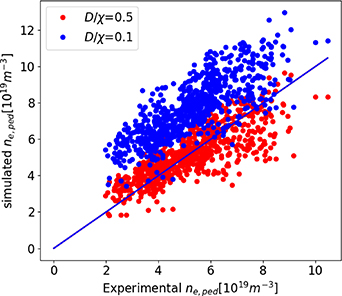
Figure 1. The testing of the standalone pedestal density modelling against the experimental pedestal density using the ionization model ignoring the KBM transport for two values of  0.5 (red, RMSE = 20%) and 0.1 (blue, RMSE = 60%). The blue line represents the perfect prediction.
Download figure:
Standard image High-resolution imageThe ideal MHD  ballooning mode limit in JET geometry is at about
  Taking into account that the KBM limit is generally lower than that of the ideal MHD limit and that we are using the average value in the pedestal, we use
  in the
  model, expression (25). Based on the considerations in [7], we choose
  = 0.3 but recognize that the model is not very sensitive to this value, provided it is sufficiently large that the main effect of the KBM transport is to force the pedestal pressure gradient to be close to the KBM limit.
Figure 2 shows the model results for two values of ETG particle transport,  0.5 and 0.1. When compared to figure 1, we can see that the
  0.5 case is hardly affected, meaning that most of those cases were below the KBM limit already. The
  0.1 case is strongly affected, matching much better with the experimental values. We obtain very good agreement between the model and experiment for both cases (the RMSE = 17% for
  0.1 and the RMSE = 15% for
  0.5). Increasing
  further to 1.0 changes the result very little from figure 2, indicating that at sufficiently high
  the pedestal
  is limited close to the KBM limit. The contribution of different components to
  naturally vary as the parameters are changed with the KBM part contributing 10%–20% with
 0.5 and 30%–60% with
  with most of the rest covered by the ETG. The NC contribution is always the smallest. Within one set of parameters, the KBM contribution decreases with the height of the density pedestal.

Figure 2. The testing of the standalone pedestal density modelling against the experimental pedestal density using the ionization model with KBM transport ( = 0.3 and
  for two values of
  0.5 (red, RMSE = 17%) and 0.1 (blue, RMSE = 15%). The blue line represents the perfect prediction.
Download figure:
Standard image High-resolution image3.2. Europed modelling
Europed is an implementation of the EPED model [2] that includes several extensions outlined in [15]. The EPED model predicts the pedestal plasma profiles given a set of input parameters (plasma shape, toroidal field, plasma current, global  , pedestal and separatrix densities). Most of them can be known in advance of the experiment. However,
  , pedestal and separatrix density are not necessarily known. The Europed extensions in [15] tried to predict these values by using inputs such as heating power and fuelling rate. While the results were encouraging, the model for the density pedestal prediction was very specific for JET and most likely does not generalize to other tokamaks. Further, it produced the opposite dependence on the isotope mass from what was seen in the experiment.
Therefore, in this work it is replaced with the model outlined above. In the full model, the density prediction is combined with the EPED constraint  , where
  is the width of the pedestal in normalized poloidal flux, c is a constant (c = 0.076 in the EPED1 model) and
  is the poloidal
  at the top of the pedestal. This constraint is used to calculate the temperature pedestal for given
  and the corresponding density pedestal calculated by the ionisation model described above. In practice this is implemented by iterating between the calculation of density profile using a known temperature profile as in section 3 and calculating the temperature pedestal profile using the EPED constraint. The above procedure is done for a range of different values of
  to produce a set of pedestal profiles and equilibria that are consistent with the EPED constraint and density pedestal model. Finally, the peeling-ballooning stability calculation is used to select the pedestal that is marginally stable as the final prediction. In the density pedestal model of Europed, we use the same parameters as in the standalone model. We also test the sensitivity of the model results to the input parameters. The modelling is done in a similar manner to [15], except that we use the new bootstrap current model by Redl introduced in [14] that is shown to work better than the Sauter model used in [15] at high collisionality, but it was not available when the modelling of [15] was done.
We first test the model without the KBM particle transport (i.e.  . Using the value of
 , we obtain the result shown in figure 3 with RMSE = 20%. The scatter of the data is slightly worse than with the standalone model that uses the experimental temperature profile.
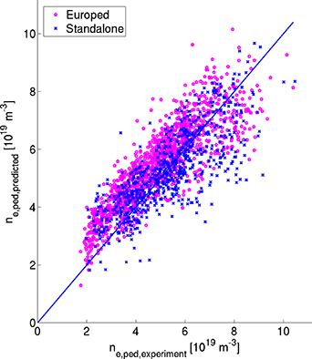
Figure 3. The comparison of the prediction of the pedestal density against the experimental pedestal density using the ionization model ignoring the KBM transport and assuming  0.5 for the full Europed modelling (magenta, RMSE = 20%) and standalone model with experimental temperature (blue, RMSE = 28%). The blue line represents the perfect prediction.
Download figure:
Standard image High-resolution imageNext, we include the KBM transport and decrease the ETG particle transport, which was found to improve the fit in the standalone model. We use the following parameters  ,
,  Unlike in the standalone model, with the full Europed model we get a worse match with the experiment, as shown in figure 4. In particular, the low experimental values of
  are under predicted This is the case, despite the Europed modelling being performed with a relatively modest KBM transport assumption, compared to what was used with the standalone model.

Figure 4. The comparison of the prediction of the pedestal density against the experimental pedestal density using the ionization model including the KBM transport with the parameters  ,
,  ,
,  0.2 using full Europed (magenta, RMSE = 26). For comparison the standalone predictions with the same parameters are shown (blue, RMSE = 20%). The blue line represents the perfect prediction.
Download figure:
Standard image High-resolution imageThe optimal result is achieved with a very small KBM component of the particle transport ( ), combined with a relatively large ETG component (
  ), although the improvement over the modelling without any KBM transport is small (RMSE = 19%).
We compare this final model to the model predictions in [15] that used a simple neutral penetration model:
where  is the velocity of the neutrals,
  is the flux expansion ratio between the fuelling location and the midplane and
  is the pedestal width, while other quantities are as above. Although in [15]
  was found to depend on triangularity, this has little physics basis and was only included as it improved the fit with the experiment. Nevertheless, we compare the new model results with the old model run with
  (where
  is the gas fuelling rate in units of
  electrons/s and
  is the triangularity).
As can be seen in figure 5, the model performs similarly at medium densities to the model used in [15] which has an RMSE = 25%, but is in better agreement with the experiment, both at high and low density.
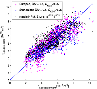
Figure 5. The comparison of the prediction of the pedestal density against the experimental pedestal density using the ionization model including the KBM transport with the parameters  ,
,  ,
,  0.5 using full Europed (magenta stars, RMSE = 19%) and the standalone (blue crosses, RMSE = 18%). For comparison the predictions using the simple neutral penetration model in [15] are shown (black dots, RMSE = 25%). The blue line represents the perfect prediction.
Download figure:
Standard image High-resolution imageThe significant difference between the full Europed prediction compared to that of the standalone model is that the fit of the predicted to experimental data is significantly worse when the KBM transport is included than when it is not. Of course, it must be noted here that the model with the fixed  value, regardless of, for instance, the role of magnetic shear in the pedestal that has been found to affect KBM stability may be too crude for this model, and a better result could be obtained by using the ideal MHD,
  ballooning mode stability limit as a proxy for KBM stability limit, but that is left for future work.
One explanation for this behaviour of the pedestal density prediction is that the KBM constraint is already included in the EPED model used in Europed. This leads to a feedback loop in the iteration, where the model increases  when a particular pedestal exceeds
  . This leads to a lower density pedestal, which is then compensated in the model by increasing
  (to keep
  fixed for the given temperature pedestal width), which then returns the value of the pedestal
  to above
  , and the density is then reduced even further. This could be avoided in the future development of the model if the EPED criteria for the pedestal pressure is replaced by a criterion for the temperature profile (e.g.
  = constant as used in [17]) that is independent of the pedestal pressure. Another option is to use a stiff ETG turbulence-based model where
  [7, 16], where
  . However, this model may suffer the same kind of internal instability as the EPED model as the temperature profile depends on the density profile, which in turn depends on the temperature profile. Furthermore, it uniquely defines both profiles, which makes the peeling-ballooning constraint irrelevant. A possible way to include it would be to make
  the free parameter (similarly to
  in the EPED model) and choose the pedestal profile associated with the value of
  that corresponds to marginal stability.
4. Sensitivity of the model
While the model is able predict the experimental behaviour remarkably well when using experimental parameters, it still has some sensitivity to the input parameters that are not known before the experiment; in particular, the separatrix density used for the boundary condition for the prediction model can strongly affect the pedestal density prediction. Figure 6 shows the dependence of the pedestal density prediction on the separatrix density for a sample case where the experimental pedestal density was predicted accurately. Since the pedestal density prediction is so sensitive to the separatrix density, the predictions using this model should be integrated with a full SOL model or at least with a simple separatrix density model such as that used in [17], where the separatrix density is connected to the neutral pressure at the divertor, which in turn can be calculated from the known gas fuelling rate, heating power and divertor pumping speed. However, this method may not work for a device for which we have no prior data (such as ITER), in which case the only option is the full SOL modelling. It must be noted that since the gas fuelling rate can be adjusted during the experiment,  may not have to be fully predicted but can be adjusted to a desired value with a feedback system to a gas fuelling system.
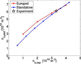
Figure 6. The pedestal density prediction as a function of assumed separatrix density using the standalone model with the experimental  profile (blue) and the full Europed model (red). The star represents the experimental case.
Download figure:
Standard image High-resolution imageThe other parameter in the model that we need to make assumptions about, is the Franck–Condon neutral density at the separatrix,  . Figure 7 shows that the model is relatively insensitive to this parameter and an order of magnitude change from
  to
to  in
in  changes the
  prediction only by about 20% in the full Europed simulation. We can also see that the dependence of
  on
on  is linear in both the standalone and Europed models.
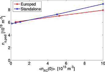
Figure 7. The pedestal density prediction as a function of assumed Franck–Condon neutral density at the separatrix  .
.
Download figure:
Standard image High-resolution imageThe poloidal distribution of the Franck–Condon neutrals that is modelled using the parameter  could be lower than 1 if most of the neutrals enter through X-point where the flux surfaces are further apart than on average on the separatrix. The effect of lowering
  is similar to that of changing
  .
.
5. Isotope effect
In the JET experiments it has been found that with a similar gas rate and heating power, the plasmas with hydrogen have lower pedestal density than those with deuterium [18]. In the model presented in this paper, the isotope mass enters explicitly only through the velocity of the neutral particles ( and
and  ). As both are
  , they are higher for hydrogen than for deuterium. The ion mass effect can be investigated by running Europed with the density prediction model and changing only the main ion mass in the simulation for a hydrogen plasma (JET-ILW discharge #91554). This result is shown in figure 8. As expected, the change of the isotope from hydrogen to deuterium while keeping everything else fixed decreases the pedestal density prediction. However, the change of the isotope mass is not the only thing that changes in the JET experiment. In addition, the separatrix density is lower in the hydrogen than in the deuterium experiment [18]. As shown in figure 8 when we use the
  from the deuterium case that was performed with the same power (84796), the predicted
  increases by more than what the pure isotope effect causes. Both the deuterium and hydrogen cases are well predicted when the experimental
  is used. This is because the model is sensitive to
  , with the prediction of
  decreasing with decreasing
  .
.
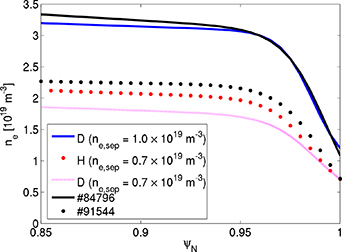
Figure 8. Europed predicted density profiles for JET-ILW hydrogen discharge 91554 assuming  from the experiment and hydrogen plasma (dotted red),
  from the experiment and deuterium plasma (magenta),
  from the equivalent deuterium discharge, 84796 and deuterium plasma (blue solid) and the profile from the experiment (91554, dotted dashed, 796 black solid).
Download figure:
Standard image High-resolution imageFurthermore, to reach the same value of global  , more heating power is required in the hydrogen plasma [18]. This means that with the same global
  the hydrogen plasma will have a larger value of
  in the model, and even with a fixed value of the
  ratio, the particle transport in the model increases with increased heating power, which in turn leads to a lower predicted
  in hydrogen. If the
  ratio also increases as suggested by the EDGE2D-EIRENE modelling [18] and non-linear gyrokinetic simulations [19] of the isotope experiments, this further lowers the predictions in hydrogen.
We ignore the possible increase of the  ratio but use the experimental
  and heating power in the modelling of the hydrogen plasmas. With these assumptions, the hydrogen cases are only slightly over-predicted compared to the deuterium ones. This is shown in figure 9 for both the standalone and full Europed models. As can be seen, both the experimental and predicted
  are lower for the hydrogen plasmas than in the deuterium plasmas. The RMSE is 32% for the standalone and 38% for the Europed predictions for the hydrogen plasmas. Finally, on doubling
  (black points in figure 9) the models predict the hydrogen cases with RMSE = 19% (standalone) and 27% (Europed).
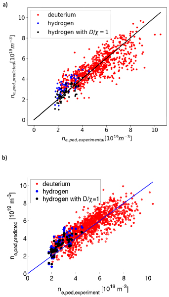
Figure 9. The predicted pedestal densities using the standalone model with experimental temperature profiles (a) and the full Europed model (b) for deuterium (red, RMSE(standalone) 18%, RMSE(Europed) = 19%) and hydrogen (blue, RMSE(standalone) = 33%, RMSE(Europed) = 38%). The model parameters for both isotopes were  ,
,  ,
,  0.5. The hydrogen case is also predicted using
  1 (black, RMSE(standalone) = 18%, RMSE(Europed) = 27%).
Download figure:
Standard image High-resolution image6. Conclusions
We have extended the ionisation model for the density pedestal presented in [5] in two ways:
- (i)We permit a core density gradient, a more realistic situation, which unfortunately prevents a simple analytic solution of the resulting second order differential equation as presented in [5], so that a numerical solution is required.
- (ii)Stimulated by techniques in [6] we include a self-consistent population of charge exchange neutrals. This results in a fourth order system of differential equations, thus requiring four boundary conditions, which can be taken to be the influx of neutrals, the core electron radial density gradient and the separatrix electron density and its gradient. An analytic integration reduces this to a non-linear third order differential equation, but an alternative formulation, an iterative solution to a second order equation, is described. In addition to the boundary conditions, the solution requires only a model for the particle diffusion in the pedestal.
We have incorporated the density prediction model both as a standalone model using experimental temperature profiles and in the Europed approach that predicts both the density and temperature pedestals. Both models use the required particle diffusion coefficient arising from ETG and KBM turbulence together with a small NC contribution. In testing it against the JET-ILW pedestal database, we find:
- (i)The full pedestal modelling with the Europed model for the pedestal pressure, reasonable assumptions for the SOL neutrals and assuming that the particle transport coefficient is tied to the heat transport in the pedestal, can predict the pedestal density for JET-ILW to high accuracy throughout the pedestal database. Including a strong KBM component with the transport increasing rapidly after the stability limit is crossed, gives good predictions with the standalone model, but leads to too much transport in the full Europed model due to the underlying pedestal pressure model that keeps the pedestal pressure gradient fixed for a given pedestal width.
- (ii)The density pedestal prediction is sensitive to the boundary condition
 , which is not an engineering parameter. This means that for a full pedestal profile prediction, the model needs to be integrated with a SOL model that can predict the value of .
 - (iii)The full model can predict the experimentally observed isotope effect in the pedestal density, even though the isotope effect on the neutral penetration alone is opposite to the observed trend. This is due to the sensitivity of the model to as well as the decreasing particle transport in the pedestal with isotope mass.


To further improve the predictive capability of the model presented here requires coupling it with a SOL model that could predict  using only engineering parameters such as the divertor configuration and gas fuelling rate. The model should also be tested against experimental data from other devices to determine the robustness of the parameters used in it. An alternative to the EPED modelling of the temperature profiles would be to use a physics-based thermal transport model involving, say, ETG and KBMs, together with ion NC transport, thus providing a complete model for predicting pedestal characteristics. A simpler alternative would be to use stiff transport models for ETG and KBMs for the temperature profiles.
Acknowledgments
The authors would like to thank James Simpson for fruitful discussions during the course of the work.
This work has been carried out within the framework of the EUROfusion Consortium, funded by the European Union via the Euratom Research and Training Programme (Grant Agreement No. 101052200—EUROfusion). Views and opinions expressed are however those of the author(s) only and do not necessarily reflect those of the European Union or the European Commission. Neither the European Union nor the European Commission can be held responsible for them.
This work has been part-funded by the EPSRC Energy Programme (Grant Number EP/W006839/1). To obtain further information on the data and models underlying this paper please contact PublicationsManager@ukaea.uk*.
For the purpose of open access, the author(s) has applied a Creative Commons Attribution (CC BY) licence (where permitted by UKRI, 'Open Government Licence' or 'Creative Commons Attribution No-derivatives (CC BY-ND) licence' may be stated instead) to any Author Accepted Manuscript version arising.