


Abstract
We present a uniquely fast (10 μs) ion temperature measurements in the tokamak edge plasma. Our approach is based on the sweeping of a ball-pen probe, where the ion temperature is obtained by fitting the electron branch of the corresponding I–V characteristic. We have performed measurements on the COMPASS tokamak during L-mode discharge. The temperature histograms reveal a non-Gaussian shape with a high-temperature tail peaking at low values. The fitted values of fast I–V measurements can be used to reconstruct (emulate) the slow swept I–V characteristic of a retarding field analyzer. The resulting ion temperature profile is nearly flat and provides a ratio of ion to electron temperature close to 1–2 in the vicinity of the last closed flux surface during L-mode discharges, as observed on other tokamaks.
Export citation and abstract BibTeX RIS
1. Introduction
The ion and electron temperatures, Ti and Te, are essential parameters of magnetic fusion devices. The ion energy is crucial especially for physical sputtering of the tungsten material of plasma facing component [1]. The edge electron temperature is commonly measured by probe diagnostics with high and low temporal resolution [2–5]. Conversely, ion temperature measurements are typically limited to a few kHz using e.g. a retarding field analyzer (RFA) [6–9]. Applying a fast-swept voltage to this diagnostic is challenging because the measured current—on the level of tens of microamps—is very small compared to the parasitic current of the coaxial cable. For example, 100 V at a frequency of 50 kHz causes ∼30 mA of parasitic current over a 5 m coaxial cable. However, recent measurements on ASDEX Upgrade using RFA with a higher sweeping frequency of 10 kHz [8] show that only fast sweeping should be used in intermittent scrape-off layer (SOL) plasmas for an accurate reconstruction of the ion temperature histograms.
Another possibility to measure the ion temperature is to use the Katsumata probe [10]. This probe technique has a high effective signal, but it requires sweeping both the collector and the metal shielding tube [10, 11]. This needs a complex isolation of the conducting parts within the graphite body of the probe head [12]. The segmented tunnel probe [10, 13] can also provide Ti with high temporal resolution. However, the interpretation of the measured signal relies on PIC simulations. Alternatively, the ball-pen probe (BPP) has a total current in the order of 100 mA [2], large enough to use sweeping frequencies of 50 kHz, and can measure the ion temperature without a complex insulation system or the need for simulations. The sweeping frequency 50 kHz (10 μs per I–V characteristic) is already within the range of the typical blob autocorrelation time (10–20 μs) on COMPASS (figure 2 in [14]).
Its simple build [15] is designed to capture the ions by leveraging their larger gyro-radius as compared to the electrons. Nevertheless, detailed 3D PIC simulations have shown that it is the E × B drift, which mainly transports particles towards the collector [16]. Some of the electrons are therefore collected, resulting in a symmetric I–V characteristic [2, 17] where the floating potential (ΦBPP) is approximately equal to the plasma (space) potential. In the following we assume that the electron branch of the BPP characteristic is the sum of the ion current, exponentially decaying with coefficient Ti, and the electron current, saturated or linearly increasing with the applied voltage. The ion temperature Ti can thus be obtained with high temporal resolution by fitting the exponential part of the electron branch.
2. Experimental setup and description of the method
A fast reciprocating probe head (see figure 1) [2], with ball-pen and Langmuir pins, is installed at the COMPASS midplane manipulator and inserted into the SOL during L-mode discharges. The BPP have stainless steel collectors with a diameter of 2 mm and an alumina shielding with inner diameters of 5 mm. The Langmuir pins are made of graphite (0.9 mm in diameter) and protrude 1.5 mm into the plasma. The averaged reciprocation time is roughly 150 ms. BPP3 is biased with a voltage of 0 to +140 V, at a sweeping frequency of 50 kHz, via a 5 m coaxial cable (parasitic capacity 100 pF m−1). The data is collected with a sampling rate of 5 MHz.

Figure 1. Probe head with three BPPs and two Langmuir probes. BPP3 is biased by a sweeping voltage at 50 kHz.
Download figure:
Standard image High-resolution imageThe electron branch of the BPP characteristic is measured when the bias voltage is above the plasma potential Φ. The probe current is there described by a general formula for non-saturated I–V characteristics, where the former term gives the linear growth of the electron current, while the latter corresponds to the exponential decay of the ion current.

The values  and
and  represent the electron and ion saturation currents, respectively. The coefficient K represents the slope ΔI/ΔV of the non-saturated part of the I–V characteristic. Such a linear coefficient is routinely used to account for sheath expansion in fitting the non-saturated ion branch of Langmuir probe I–V characteristics, equation (2) in [18]. The linear increase of the electron current has been reproduced in PIC simulations (chapter 4 in [16]) and awaits theoretical explanation. The coefficient K is equal to 0 when the electron current is fully saturated above Φ. We introduce the ratio between the electron and ion saturation currents

For the BPP measurements, a value of αBPP = 0.6 can be used on COMPASS [2], as well as AUG [17]. The combination of the equation (1) and (2) leads to a general four-parameter fitting formula of the electron branch of the BPP I–V characteristic
Previous work on AUG [19] used a three-parameter fitting formula, with K = 0, and the assumption that  =
=  . However, it was found that in many cases the electron branch is not fully saturated (K > 0) and that the strict application of three-parameter fitting lead to an overestimation of Ti. The probe head can also simultaneously provide Te, with high-temporal resolution, combining the floating potentials measured by LP1 (Vfl
LP) and BPP2 (ΦBPP):
. However, it was found that in many cases the electron branch is not fully saturated (K > 0) and that the strict application of three-parameter fitting lead to an overestimation of Ti. The probe head can also simultaneously provide Te, with high-temporal resolution, combining the floating potentials measured by LP1 (Vfl
LP) and BPP2 (ΦBPP):

This technique is routinely employed on COMPASS (αLP = 2.8) [2, 20] and has been used on AUG, MAST and ISTTOK [2, 21–23].
3. Ion temperature profile measurements with 10 μs resolution
The main obstacle for high temporal resolution RFA measurements is the instrument's very low effective signal—in the order of tens of μA [6, 7]. This is generally incompatible with the large capacitive currents (tens of mA) caused by high sweeping frequencies. This problem can be overcome using BPP technique as it provides high enough effective signal. The capacitive current is typically reconstructed from the time derivative of the voltage and current measurements before the tokamak discharge. The reconstructed parasitic current is then subtracted from the current measurements during the whole discharge. This process reduces the parasitic contribution to the total current by a factor of 6 or 7. We also apply a lowpass filter to remove the frequencies above 370 kHz. The probe current and voltage are then split into individual I–V characteristics and fitted by equation (3). One difficulty is that the model is only valid for the electron branch (V > Φ). Therefore, a first fit must be used to find the plasma potential, using all positive current values above the BPP floating potential. The fitting process is then repeated for current values strictly above the obtained plasma potential. All fittings use the least square technique with a weighing factor of 1/σ, as shown in figure 2. The value σ of each point of the I–V characteristic is obtained as a standard deviation of all current fluctuations around the probe voltage +/−1 ms. We also check if the voltage range above the plasma potential is equal or larger than 3Ti where the linear part of the I–V characteristic starts to dominate. When this is not the case, a new iteration is done for which the four-parameter fitting formula is reduced to three-parameter (K = 0) to re-fit the I–V characteristic without the linear part. Following this approach, we analysed the measurements performed during L-mode discharge #7029 (BT = 1.15 T, IP = 170 kA, ne = 5 × 10¹⁹ m−3) with density on last closed flux surface (LCFS) ne,LCFS ∼ 1 × 10¹⁹ m−3 obtained by Li-beam diagnostic [24]. The resulting SOL ion temperature profile (Ti obtained every 10 μs), with a maximum relative error 60%, is plotted in figure 3. The graph also shows Te with the same lowpass filter. The radial position of the probe head is plotted with respect to the position of the LCFS, routinely obtained on COMPASS [2] by finding the maximum of the plasma potential profile, where the electric field E = − grad(Φ) and the corresponding E × B flow is zero. It is evident that the Ti measurements are scattered rather than forming a clear profile. An example of the Ti and Te temporal evolution from within the near SOL (R − RLCFS ∼ 0.001 m) and main SOL (0.012 < R − RLCFS [m] < 0.014 m) region is shown in figure 4. The electron temperature is plotted with high temporal resolution as well as with points corresponding to the time of Ti measurements. It is important to stress that Ti and Te measurements are performed at different poloidal locations (displaced roughly by 15 mm on the probe head). Thus, the same event (blob) will be observed by Ti and Te at different time with respect to its poloidal velocity (figure 9 in [25]). Note that the successfully obtained Ti values represents roughly 30% of all measured I–V characteristics. Thus, we can only see part of the temporal evolution with high resolution. The reason might be that the sweeping frequency is still not high enough to catch all blobs with shorter period and consequently the I–V characteristics are strongly deformed.

Figure 2. Electron branch (V ⩾ Φ ≈ 35 V) of a single-sweep BPP characteristic fitted by equation (3) using least-square minimization weighing each point by 1/σ.
Download figure:
Standard image High-resolution image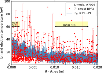
Figure 3. Radial profile of Ti and Te. The position of the probe is shown on the x-axis with respect to the coordinate of the LCFS in the outer midplane. For clarity, the absolute error bars are only shown for a few points.
Download figure:
Standard image High-resolution image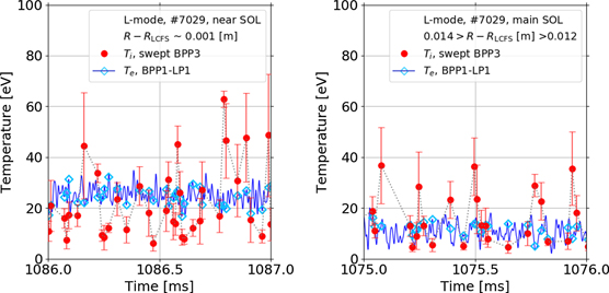
Figure 4. Example of the temporal evolution of Ti (red circles) and Te (blue line and diamonds) in the near SOL (left) and in the main SOL (right). The electron temperature is plotted with high temporal resolution (line) and with points (diamonds) corresponding to the time of Ti measurements.
Download figure:
Standard image High-resolution imageThe Ti and Te histograms for the near SOL (0 < R − RLCFS [m] < 0.002) and the main SOL (0.01 < R − RLCFS [m] < 0.018) regions are shown in figure 5. The Ti histogram has a non-Gaussian shape peaking at ∼10 eV, with a large tail up to ∼55 eV. The large tail may be the product of turbulent filamentary structures (blobs) [26] originating in the vicinity of the LCFS and propagating through the entire SOL. The low values may be attributed to the background plasma (figure 12 in [7]) and the impurity content [27]. These low values are similar for ions and electrons in the main SOL. We have also observed that the level of relative fluctuation, standard deviation of the temperature normalized by its mean value, decreases towards the LCFS for both Ti and Te. It is a direct consequence of the blobby transport in SOL [2, 21, 23]. A secondary Ti maximum appears in the near SOL and corresponds to the maximum of the Te histogram.
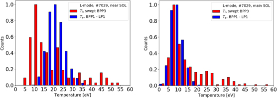
Figure 5. Ion and electron temperature histograms for near SOL (left) and main SOL (right) locations in shot #7029.
Download figure:
Standard image High-resolution image4. Ion temperature profiles from RFA-like I–V characteristics (low resolution)
In order to show an averaged profile, similar to a slow swept RFA, we have reconstructed the slow-swept RFA-like characteristics with period 3 ms using the fitted parameters obtained with the fast-swept BPP. The fitted values of Ti, Φ and Isat + from fast BPP measurements are used to reconstruct the RFA characteristic using the functional form:
These reconstructed I–V characteristics are then averaged over 3 ms intervals to create one slow (RFA-like) I–V characteristic of pure ion current, as shown in figure 6. The ion current decay in logarithmic scale, starting from the vicinity of the averaged plasma potential Φ ∼ 38 V, is fitted by a linear function with a current cut-off (Isat +/e) corresponding to roughly 37% of the nominal Isat + [27]. The result is that only the tail of the I–V characteristic is taken into account.
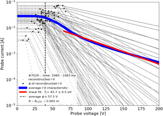
Figure 6. I–V characteristics reconstructed from fast swept BPP fittings (Ti, Φ and Isat +) over a 3 ms interval in the vicinity of LCFS (#7029). The averaged I–V characteristic is fitted with the same upper limit for collector current as shown in [27].
Download figure:
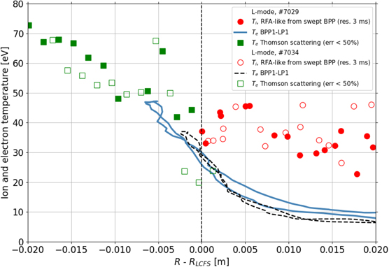
Standard image High-resolution imageThe ion temperatures obtained by the averaged (RFA-like) I–V characteristics from discharge #7029 and the complementary discharge #7034 (same plasma parameters) are shown in figure 7. The electron temperature profiles are obtained from fast BPP-LP measurements and smoothed down to the same temporal resolution and from the Thomson scattering system [28] as well. Both, Ti and Te profiles show the good reproducibility of our measurements. The resulting Ti profile does not contain any low values, apparent in figure 3. This is to be expected since the fitting procedure applied on the tail of the I–V characteristic is dominated by blob temperatures, as pointed out in [26]. However, the Ti histograms may differ if the RFA (-like) I–V characteristics are fitted with different current cut-off or voltage cut-off, as noted in [8]. We see in figure 7 that the ratio Ti/Te is larger in the main-SOL than in the vicinity of the LCFS. This was also observed on JET, KSTAR, EAST and AUG (cf figure 1 in [29]) where Ti is measured by other diagnostic systems.
Figure 7. Ion temperature profiles obtained from averaged (RFA-like) I–V characteristics (circles) in two L-mode discharges #7029 and #7034 with the temporal resolution 3 ms. The electron temperature profile in SOL is obtained from fast BPP-LP measurements (line) and smoothed down to the same temporal resolution and Thomson scattering system (squares). The limiter is located around R − RLCFS = 0.02 m.
Download figure:
Standard image High-resolution image
5. Conclusion
We used the fast swept BPP technique to obtain fast measurements (every 10 μs) of the ion temperature during L-mode tokamak discharges on COMPASS. The BPP I–V characteristics are fitted by a four-parameter formula providing Ti, Φ and Isat +. The resulting temperature histograms have a non-Gaussian shape with a peak at low temperatures and a tail towards high temperatures. This feature is observed in the near SOL as well as the main SOL. The large tail Ti values might be attributed to the filamentary turbulent structures (blobs) originating at the vicinity of LCFS and propagating through the SOL. The low values may correspond to the background plasma and the impurity content. In order to obtain an ion temperature profile with very low temporal resolution (similar to a slow swept RFA), we have used an averaged RFA-like I–V characteristics with the period 3 ms using fitted values of Ti, Φ and Isat + from fast BPP measurements. The resulting ion temperature profile is nearly flat and provides the ratio of ion to electron temperature close to 1–2 in the vicinity of the LCFS as it is observed on other tokamaks (JET, KSTAR, EAST, AUG).
Fast swept BPP technique reveals a broad spectrum of Ti values with the blob and background temperatures as similarly observed by recent RFA measurements on MAST and AUG, albeit a significantly higher temporal resolution. It is clear that the slow swept technique combines all these Ti values within a single I–V characteristic causing a difficult interpretation of the measurements. The BPP technique is robust and simple and features a very high effective signal allowing for Ti measurements at the edge of magnetic fusion facilities. It is reported in this work that we were able to successfully obtain 30% of all available data with 50 kHz sweeping frequency (5 MHz sampling frequency). Thus, with an even higher sweeping frequency (∼100 kHz) this diagnostic should be able to 'catch' more blob events with typical autocorrelation time 10–20 μs as shown for COMPASS (figure 2 in [14]). It is worth mentioning that using slow sweeping frequency (∼1 kHz , typical for RFA diagnostic) we would deliver only several points per 1 ms. Thus, our fast measurements resolve more data than it is typically achieved for Ti measurements.
Acknowledgments
The first author would like to thank M. Peterka for initial discussions on the fitting routines. This work has been carried out in the framework of the EUROFusion Consortium and has received funding from the Euratom research and training programme 2014–2018 and 2019–2020 under Grant agreement No. 633053. The views and opinions expressed herein do not necessarily reflect those of the European Commission. This investigation was supported projects MEYS #LM2018117, CZ.02.1.01/0.0/0.0/16_019/0000768 and IAEA CRP F13019 - Research Contract No. 22727/R0. This work was also supported by the Czech Science Foundation within the project GACR 20-28161S and 19-00579S.