
Abstract
Analysis of heat fluxes in scrape-off layer (SOL) plasma is important for the prediction of divertor tile heat loads in future reactor-sized tokamak machines. Typically, the radial heat flux profile can be accurately characterized by the decay length parameter λq. The predictions are then based on the dependence of λq on plasma and machine parameters. In recent years, several empirical scaling models were derived from a collective database of decay lengths observed in several large tokamaks as well as two spherical tokamaks. Most recently, a report from the TCV tokamak showed a deviation from several of the proposed models (Maurizio et al (TCV team) 2021 Nucl. Fusion61 024003). In this work,  edge plasma profiles of ELMy H-mode discharges were collected from the COMPASS tokamak database for heat flux analysis. The COMPASS tokamak has a similar machine size and plasma parameters to the TCV tokamak, offering a valuable comparison. The λq was measured in both downstream and upstream SOL utilizing a divertor probe array validated by an IR camera and Thomson scattering diagnostics. A comparison with the predictions of several scaling models indicated an occurrence of anomalously short (by a factor of 2–5) inter-ELM power decay lengths in both upstream and downstream, as well as a difference in λq between these two regions. Possible causes related to the accuracy of magnetic reconstruction were eliminated and physics-based sources of apparent compression effects were hypothesized as a motivation for future research.
Export citation and abstract BibTeX RIS

Original content from this work may be used under the terms of the Creative Commons Attribution 4.0 license. Any further distribution of this work must maintain attribution to the author(s) and the title of the work, journal citation and DOI.
1. Introduction
Divertor tiles are plasma-facing components of a tokamak which may be exposed to extremely high heat and particle fluxes transported by the plasma particles. The research of the power exhaust becomes crucial in the light of future reactor-sized machines. The current state of knowledge in the area of magnetic confinement fusion suggests favourable scaling of the confinement time with machine size. The next generation of tokamaks is to surpass all of the current experiments in both the physical scale and the economic burden. The design of such machines necessitates accurate predictions of heat fluxes that would allow specifying realistic material and structural requirements of critical plasma-facing components.
In recent years, a database of measured divertor heat fluxes in H-mode discharges was collected from multiple tokamaks [1–4] and collectively analyzed with the aim of providing predictions for ITER tokamak and next-step devices. The analysis was focused on the divertor heat flux profile, which is typically characterized by the heat flux decay length λq [5].
A regression analysis of the decay length data revealed a set of plasma parameters that appear to have a significant effect on the magnitude of λq
. These parameters include, most notably, the poloidal  and toroidal
  magnetic fields, the mean plasma pressure
  [3] and the edge plasma pressure p95 [4]. Several empirical scaling models were proposed and tested, yielding promising results in decent agreement with available experimental data. The models are based on a multi-machine database, which includes data from several large conventional tokamaks as well as from two spherical tokamaks, which feature a very low aspect ratio
  . Note that the latter group represents a significant part of the database, as it covers a specific corner of the parameter space with small machine size and low performance parameters (low pressure, low
  , etc), and thus it has a strong impact on the results of the regressions.
Pursuing the topic further, a recent 2021 report by Maurizio et al [1] presented results from the TCV tokamak, which exhibited a disagreement with predictions of a number of multi-machine scaling laws. Based on its dimensions and its  magnitude, TCV covers a similar region of the parameter space as the spherical tokamaks from the multi-machine database; however, it features on average two to three times shorter decay lengths λq
. Maurizio states that a reasonable agreement was found only when both the power crossing the separatrix
magnitude, TCV covers a similar region of the parameter space as the spherical tokamaks from the multi-machine database; however, it features on average two to three times shorter decay lengths λq
. Maurizio states that a reasonable agreement was found only when both the power crossing the separatrix  and the Greenwald density fraction
  were included in the scaling model.
The COMPASS tokamak (R = 0.56 m, a = 0.18 m,  –2.1 T, κ = 1.6, plasma current up to 400 kA, NBI heating
  ) is a machine with dimensions and discharge parameters close to the TCV tokamak. Therefore, it was deemed to be an ideal candidate to help disentangle the role of small machines vs spherical machines in view of the scaling models and the λq
predictions. In 2020, Horacek et al [6] conducted research of λq
scaling in COMPASS L-mode discharges. This paper contributes further to the topic by presenting an analysis of the inter-ELM λq
in ELMy H-mode discharges.
) is a machine with dimensions and discharge parameters close to the TCV tokamak. Therefore, it was deemed to be an ideal candidate to help disentangle the role of small machines vs spherical machines in view of the scaling models and the λq
predictions. In 2020, Horacek et al [6] conducted research of λq
scaling in COMPASS L-mode discharges. This paper contributes further to the topic by presenting an analysis of the inter-ELM λq
in ELMy H-mode discharges.
The outline of this work starts with section 2, which introduces the diagnostic systems and methods that were used to measure the plasma profiles. The process of discharge selection suitable for the analysis is described in section 3 together with the decay length fitting methods and an overview of the resulting database. An analysis of the results and a comparison with previous findings in the TCV tokamak and other machines are presented in section 4. Finally, the conclusions drawn from the COMPASS observations and proposals for future work are discussed in section 5.
2. Experimental methods
The most common diagnostic systems for observing the divertor heat flux profiles include the infra-red (IR) camera systems [7, 8], the array of divertor probes [9] and the Thomson scattering (TS) diagnostics [10], which are all available on the COMPASS tokamak. An overview of the physical regions observed by the respective diagnostics is shown in figure 1. The focus of this work is on the power decay length λq , which is by convention mapped and measured at the outer midplane (OMP). The parameters and the involvement of each diagnostic in this analysis are described in the dedicated subsections below, whereas the calculation of λq is addressed in section 3.
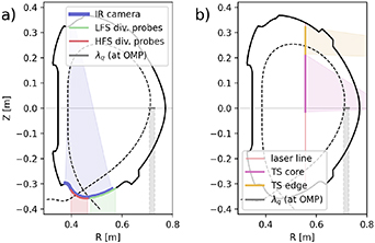
Figure 1. A schematic view of the regions observed by the edge diagnostics in the COMPASS tokamak. The divertor target, (a), is observed both by the array of divertor probes and by the IR camera. The upstream SOL, (b), is observed by the Edge TS diagnostics in the upper section of the vacuum vessel. Heat flux decay length λq is measured at the outer midplane (OMP).
Download figure:
Standard image High-resolution imageHeat flux profiles were observed during an ELMy H-mode phase of a discharge in the time between two adjacent ELM events, often referred to as the inter-ELM phase. As shown, for example, in [11], in the late part of the ELM cycle, which precedes the ELM crash, the pedestal gradients tend to saturate. This can be exploited to establish well-defined and consistent measurement conditions. For the purpose of this experiment, a time range of 70%–85% of an ELM cycle (peak-to-peak) was used. This choice was a compromise between measuring as saturated profiles, as possible, on the one hand, and avoiding the rising edge of the next peak together with any occasional precursor fluctuations, on the other hand. The situation is illustrated in figure 2.

Figure 2. An example plot of the D radiation intensity showing the typical peaks caused by the ELM crashes and the definition of the inter-ELM interval (red markings), during which the power decay lengths were observed.
Download figure:
Standard image High-resolution image2.1. Downstream diagnostics: divertor probe array
The COMPASS tokamak features a combined array of ball-pen probes (BPP) and Langmuir probes (LP) [9, 12]. Pairs of BPP and LP are used to measure the radial profile of electron temperature of plasma  along the divertor target, as indicated by (a) in figure 1, with high temporal resolution (
 s). A second parallel array of LPs is employed to measure the ion saturation current
  . The physical spacing of the probes in each array is
  mm with a corresponding effective spacing at the OMP
  0.25–0.50 mm. The divertor heat flux parallel to the field lines is then calculated as
where  mm2 is the cross-section of the probe heads when projected perpendicular to the field lines used to calculate the ion saturation current density
  ,
,  is the potential energy deposited by each ion-electron pair to the target, which is equal to a sum of ionisation energy (13.6 eV for deuterium) and surface bonding energy (
 eV) [13] and γ is the sheath heat transmission factor.
In the previous works [9, 14], a fixed value of γ = 11 was assumed, which resulted from a comparison between the probe data and IR camera measurements [8]. However, recent results from ASDEX Upgrade suggested that the contribution of non-ambipolar heat fluxes can be significant and can influence the deduced λq
[15]. Therefore, we have employed a more detailed calculation of γ and  , which takes these effects into account. Following similar derivations in [15–17], the impacting heat flux
  on grounded divertor tile (
 V) can be calculated as
While the ion heat flux is given by the thermal energy of ions and their acceleration in the sheath, the electron heat flux is a product of the energy that each electron delivers to the surface (equal to  ) and the electron flux density to surface
  . In the case of LP operated with swept voltage bias, this flux can be easily obtained from the probe current density j0 at
  V
V

However, the combined probe array (BPP+LP) does not provide such measurements. Instead, it is possible to predict  using the knowledge of
  ,
,  and
and  , assuming a simple 3-parameter model of the current–voltage (I-V) characteristic [18]
The magnitude of  is constrained by the maximum electron current density, which can be drawn by the surface (which is often smaller than the theoretical limit in magnetized plasmas). Measurements of the combined probe array suggest a ratio of electron to ion saturation currents
  [9], which translates to maximum
  and subsequently γ ≈ 17 (neglecting the contribution of
  at high
  ).
).
An example profile of  and γ (assuming
  =
=  ) are shown in figure 3. It can be seen that in the vicinity of the outer strike point, the value of γ is close to the previously used value 11 and further away drops to
  , which is the value corresponding to the ambipolar conditions [16]. The limitation given by the reduced electron current is not reached. The resulting effect of the choice of γ calculation on the value of λq
is smaller than the precision of the fit (∼10
, which is the value corresponding to the ambipolar conditions [16]. The limitation given by the reduced electron current is not reached. The resulting effect of the choice of γ calculation on the value of λq
is smaller than the precision of the fit (∼10 ), nevertheless we have utilised this method of
  determination in the further analysis.
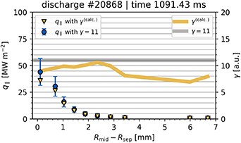
Figure 3. Example of a radial profile of the sheath heat transmission factor γ during an inter-ELM period. The γ is calculated using formulas (2) and (4). For comparison, two variants of a heat flux profile measured by the divertor probes are plotted on a secondary y-axis, one with the assumption of γ ≈ 11 and one using the calculated γ.
Download figure:
Standard image High-resolution image2.2. Validation of probe diagnostics with an IR camera
In addition to the combined probe array, the COMPASS tokamak features an IR camera system [7, 8] that observes the LFS (and HFS) divertor target from an upper port as illustrated in figure 1. Its spatial resolution ranges between 0.6–1.4 mm at the target and approx. 0.06–0.14 mm when mapped to the OMP. In its default configuration, it offers a temporal resolution of 30 µs.
In this work, the probes were favoured over the IR measurements despite the superior spatial resolution of the latter diagnostics (by a factor of 6 at the OMP). The main reason was the sparse availability of IR measurements in the studied discharges. Only a limited number of experiments offered IR data. Yet, it was still possible to demonstrate that there was no significant compromise on the data quality introduced by the use of probes. A good agreement between the two diagnostics was already demonstrated in previous works, e.g. in [8]. It was again verified here for a set of inter-ELM profiles in H-mode plasma that were more representative of the examined dataset. The results of the validation, presented in figure 4, showed a limited discrepancy between the two diagnostics. The camera λq
is systematically shorter by a factor of  (average ± std. dev.), which may be due to the limitations in processing the IR data or due to the non-negligible width of the instrument function of the probes. Nonetheless, this discrepancy presents an acceptable margin of error in the context of this work's results. The fit methods used for this validation analysis are described together with the methods for the primary analysis in section 3.
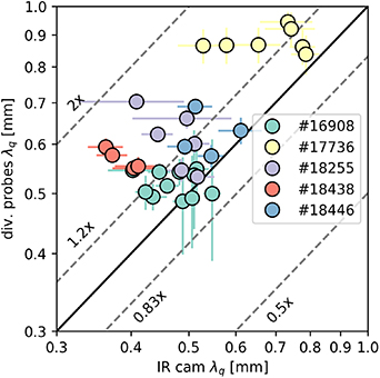
Figure 4. A comparison of the downstream λq measurements between the divertor probes array and the IR camera. The discharges represent typical H-mode discharges with quasi-stationary plasma parameters good quality of data (in respect to the probes and the IR camera) similar to those used for the main analysis.
Download figure:
Standard image High-resolution image2.3. Upstream diagnostics
Another diagnostic utilized in this work is the high resolution TS system, offering the measurements of electron temperature  and density
  in upstream. The resulting decay lengths
  and
and  were used to estimate the upstream heat flux decay length λq
according to the approximate relation introduced by Stangeby et al [19] as described later in section 3. The COMPASS tokamak features a TS setup based on solid-state Nd:YAG lasers and polychromators for fast spectral analysis [10, 20].
were used to estimate the upstream heat flux decay length λq
according to the approximate relation introduced by Stangeby et al [19] as described later in section 3. The COMPASS tokamak features a TS setup based on solid-state Nd:YAG lasers and polychromators for fast spectral analysis [10, 20].
The Edge TS observes the confined plasma in the vicinity of the pedestal and consists of 30 spatial points with spacing of  mm along the vertical laser line, see b) in figure 1. This is equivalent to an effective spacing of
  mm when mapped to the OMP. The laser pulse length during a single measurement is around 7 ns enabling measurements that are very well localised in time. On the other hand, the repetition rate of the complete four-laser system is 120 Hz yielding 1 observation per 8.3 ms, which is longer than the typical duration of an ELM cycle. This introduced complication during the formation of the λq
database is discussed in the next section.
mm when mapped to the OMP. The laser pulse length during a single measurement is around 7 ns enabling measurements that are very well localised in time. On the other hand, the repetition rate of the complete four-laser system is 120 Hz yielding 1 observation per 8.3 ms, which is longer than the typical duration of an ELM cycle. This introduced complication during the formation of the λq
database is discussed in the next section.
3. Estimating the H-mode decay lengths
A database of roughly 100 inter-ELM profiles was established. In the majority of cases, the auxiliary heating using Neutral Beam Injectors (NBI) was employed ( around 500–950 kW depending on which NBIs were active), and in some cases the plasma was heated exclusively by the ohmic power (
 around 50–400 kW). The database is divided into two datasets A and B, which differ in the TS data quality. Dataset A consists of recent discharges (year 2020) from three H-mode focused campaigns, where updated data processing routines for the TS diagnostics with better stray-light mitigation were used. Dataset B consists of earlier discharges (years 2017–2020) that were added to increase the parameter range, primarily the strength of the poloidal field
  . However, the TS data in dataset B is often affected by imperfectly mitigated stray-light effects, which results in larger fit errorbars when compared with dataset A. An overview of the total parameter space of two important scaling parameters, the poloidal magnetic field
  and the core average plasma pressure
  , is shown in figure 5, supported by a preview result of the downstream λq
measurements from the divertor probe array that are later presented in section 4.
, is shown in figure 5, supported by a preview result of the downstream λq
measurements from the divertor probe array that are later presented in section 4.

Figure 5. Histogram of the magnitude of selected discharge parameters (poloidal  and toroidal Bφ
magnetic field, average core plasma pressure
and toroidal Bφ
magnetic field, average core plasma pressure  ). Results of downstream λq
measurements from the divertor probe array (see section 4) are included in the plots to illustrate absence of strong single-parameter scaling trends.
). Results of downstream λq
measurements from the divertor probe array (see section 4) are included in the plots to illustrate absence of strong single-parameter scaling trends.
Download figure:
Standard image High-resolution imageAs mentioned in the previous section, the repetition rate of the COMPASS TS diagnostics is relatively low compared to the ELM frequency. This introduces two main drawbacks when establishing the database. First, an algorithmic scan of a wide range of prospective discharges across several campaigns was required to collect a statistically significant number of inter-ELM profiles with TS data. Second, often there were fewer than three profiles collected from a single discharge. That eliminated the option to infer decay lengths from an aggregate profile over multiple consecutive ELM events, as used e.g. in [1, 4], which could have improved the uncertainty of the profile fits.
3.1. Fitting methods to estimate the λq from downstream data
The profiles, both downstream and upstream, were mapped to the OMP using data from the EFIT equilibrium reconstruction and fitted to obtain the decay lengths.
In the case of the downstream profiles, a simple exponential function defined as

where  and
and  , was used as the fit model, see figure 6. Note that a more advanced model, introduced by Eich in [5], which accounts for the effect of the Gaussian power spreading in the divertor regions (spreading factor S), often provides better results when applied on the downstream data [2–4]. However, the spreading effect was found to be far less significant in COMPASS, with an average value of the
  ratio was smaller than 1. An example is shown in figure 6(b). During the analysis, it was observed that a significant number of individual probe profiles do not contain sufficient number of datapoints in the private region, resulting in unreliable estimates of the S parameter. The issue is specific to the use of probe diagnostics due to the inherent limitations on spatial resolution, which can be up to an order of magnitude less favorable compared to the IR camera [2–4]. As shown in figure 6(b) it was necessary to aggregate
  profiles over several ELM cycles in a single discharge, where the plasma parameters were quasi-stationary, in order to achieve a reasonable fit of the advanced model with Gaussian spreading (Eich et al [5]).
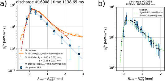
Figure 6. The left plot, (a), shows a profile of parallel plasma heat flux  measured at the LFS divertor target using the divertor probes, in blue, and the IR camera, in orange. Different variants of λq
fit are plotted in solid and dashed lines. The solid lines mark variants that were chosen for the primary analysis. The right plot, (b), shows a
measured at the LFS divertor target using the divertor probes, in blue, and the IR camera, in orange. Different variants of λq
fit are plotted in solid and dashed lines. The solid lines mark variants that were chosen for the primary analysis. The right plot, (b), shows a  profile measured by divertor probes and aggregated over several adjacent ELM cycles. This more complex approach, which was applied to a few selected discharges, enabled a stable Eich function fit.
Download figure:
Standard image High-resolution imageUnrelated to the main dataset analysis, it is also prudent to address the fit method for the IR camera data that were used solely for the validation of the probe measurements as previously described in section 2. In this case, the Eich model did not produce issues with estimating the S parameter. However, it failed to capture the experimental points in the far SOL and systematically yielded 10%–20% longer λq
values. As seen in figure 6, the  profile from the IR camera consists of two distinct exponential trends, near-SOL and far-SOL. The far-SOL data points are in strong disagreement with the divertor probes, which indicates a possible instrumental deformation due to the limited dynamic range of the camera. Since the main focus lies in the near SOL, where the bulk of the heat energy is deposited, we have used the double-lambda exponential function (double-exp) as a fit model that decouples the
  (near-SOL) and
  (far-SOL) decay lengths:
where we focus on the near-SOL decay length  . A similar approach of combining multiple exponentials with different λ parameters was previously used at Alcator C-Mod,Brunner2018. The results of the validations were presented earlier in figure 4.
3.2. Fitting methods to estimate the λq from upstream data
The upstream profiles of electron temperature  and density
  were fitted using exponential models analogous to (5)


The results can be seen in figure 7. A similar approach was used in [1, 4]. Due to the uncertainty in separatrix location and in order to increase the number of data points for the fits, we have utilised measurements outside the pedestal top, thus including some data points lying inside the separatrix. This is justified by recent observations at the ASDEX Upgrade, where it was confirmed that the density and temperature decay lengths measured inside separatrix and in near SOL are equal [21].

Figure 7. Profiles of the electron temperature  and density
  in the edge plasma measured by the Thomson scattering diagnostics. A two-point model (upstream
  ) estimate of the separatrix position is shown as a wide dashed line, its width representing the standard deviation of a 400 ms average. The solid line shows the fit of the systematically selected portion of the pedestal profile close to the separatrix. Functions (7) and (8) were used for the fit. Note that the data error bars in this figure mainly characterise the precision of the fitting routine.
Download figure:
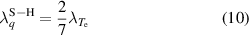
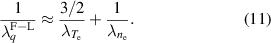
Standard image High-resolution imageAccording to Stangeby et al [19], it is possible to relate the decay lengths of radial plasma profiles (temperature  , density
  ) observed in the upstream region to the magnitude of the upstream power decay length λq
. Two different relations are formulated in [19], depending on the collisionality of the SOL electrons
) observed in the upstream region to the magnitude of the upstream power decay length λq
. Two different relations are formulated in [19], depending on the collisionality of the SOL electrons  , which can be estimated as
where  and
and  correspond to the upstream separatrix density and temperature respectively and
  is the connection length. The SOL parallel heat transport is dominated by the thermal conductivity of electrons. In the ideal collisional SOL, where
  is large, the Spitzer–Härm (S–H) conductivity is a good model for
  and provides the following relation between the decay lengths
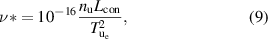
In case of weak collisionality, where  , the S–H conductivity expression fails to accurately describe the heat conduction in a quantitative sense. A more accurate description can be achieved by applying a correction (limitation) on the
  using the so called flux limiter (F-L) expression. With decreasing
  , the
, the  converges to a flux-limited description of the conduction, which yields the second relation
The divertor probe measurements allow us to calculate the upstream  using the two point model as
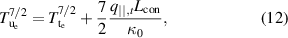
where  is the downstream electron temperature,
  is the downstream parallel peak heat flux and κ0 is the S–H electron heat conduction constant (
 eV
eV W m−1) [22]. A further analysis of the dataset showed
  eV at the outer divertor target (note that these high values were recently confirmed by analysis of swept LP [23]). As a consequence, the first term in the r.h.s. in (12) was always dominant, leading to ratio
  , thus effectively
  , which is typical of SOL in the sheath-limited regime and weak collisionality. The calculation of
  using (9) further confirmed this fact, typical values were in the range of 0.5–2 as shown in figure 8. This lead us to the decision to use formula (11), the flux-limited model.

Figure 8. Comparison of the upstream λq
analyses as calculated using the models (11) (flux-limited) and (10) (Spitzer–Härm). The colormap indicates weak collisionality in SOL, typical values of  are 0.5–2.
Download figure:
Standard image High-resolution imageIndependently of the arguments presented in the previous paragraph, figure 8 clearly shows that  is systematically shorter by 40% at maximum (30% on average), which is a smaller difference than the upstream-downstream discrepancy presented later in section 4 (factor of 2–3x, i.e. difference of 100%–200%). Thus, there is no basis for a qualitative impact on the conclusions of this work, only a limited quantitative change.
4. Results and comparison with published scaling models
A set of relevant empirical scaling models was aggregated and used for comparison with the results of this analysis, they are listed in table 1 together with references and their parameters. The complete dataset is plotted for several selected models in figure 9 to illustrate the distribution of the data points. It shows a varying amount of discrepancy between the experimental data and the models, as well as a strong discrepancy between the experimental data from upstream and downstream measurements. Since there was no strong correlation observed, the comparison with the remaining models is quantified using an average ratio of  to
to  in table 2.

Figure 9. Results of λq measured in the upstream (flux-limited assumption, see (11)) and the downstream SOL using the TS and the divertor probes, respectively, compared to selected empirical scaling models. Complete list of analysed models is in table 2. In several discharges, the probe data were additionally analysed with a more complex approach by aggregating profiles over several ELM cycles and utilizing the Eich function for the fit.
Download figure:
Standard image High-resolution imageTable 1. List of empirical scaling models for inter-ELM H-mode λq investigated in this work.
| Model | const.(mm) |
 (T) (T)
| Bφ (T) | q95[–] |
 [–] [–]
|
 (MW) (MW)
| R0(m) |
 (atm) (atm)
|
 (kPa) (kPa)
|
 [–] [–]
|
 [–] [–]
| β[–] |
|---|---|---|---|---|---|---|---|---|---|---|---|---|
| Eich #1 [2] | 0.68 | −1.07 | ||||||||||
| Eich #3 [2] | 0.65 | −1.11 | ||||||||||
| Eich #5 [2] | 0.52 | −0.92 | 0.25 | 0.10 | ||||||||
| Eich #9 [2] | 0.70 | −0.77 | 1.05 | 0.09 | 0.00 | |||||||
| Eich #11 [2] | 0.52 | −0.63 | 0.95 | 0.05 | 0.21 | −0.48 | ||||||
| Eich #14 [2] | 0.63 | −1.19 | ||||||||||
| Eich #15 [2] | 1.35 | −0.92 | –0.02 | 0.04 | −0.42 | |||||||
Brunner  [3] [3] | 0.91 | −0.48 | ||||||||||
Horacek  [6] [6] | 0.02 | −0.44 | −1.96 | −0.27 | ||||||||
| Silvagni p95 [4] | 2.45 | −0.34 | ||||||||||
| Goldston HD [24] | see equation (5) in [24] | |||||||||||
| Eich HD [2] | 0.86 | −0.80 | 1.11 | 0.11 | −0.13 | |||||||
Table 2. Comparison of λq
observed in COMPASS (upstream and downstream) and the previously published empirical scaling models, quantified by the ratio of  to
to  . The values in the table represent a mean ratio over the whole dataset ± standard deviation, model Eich #9 is marked as the best match. Full datasets are plotted in figure 9 for selected models, model definitions are in table 1.
Ratio 
| ||
|---|---|---|
| Model | upstream | downstream |
| Eich #1 [2] |

|

|
| Eich #3 [2] |

|

|
| Eich #5 [2] |

|

|
| Eich #9 [2] |

|

|
| Eich #11 [2] |

|

|
| Eich #14 [2] |

|

|
| Eich #15 [2] |

|

|
Brunner  [3] [3] |

|

|
Horacek  [6] [6] |

|

|
| Silvagni p95 [4] |

|

|
| Goldston HD [24] |

|

|
| Eich HD [2] |

|

|
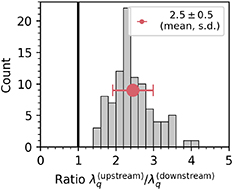
The difference between the upstream and downstream observations was further explored in a histogram in figure 10, indicating that the downstream λq is on average 2.5 times narrower. As discussed later in section 5, this effect could be explained as a result of a strong anomalous radial transport that mitigates the expansion of the heat flux profile as the SOL plasma flows towards the divertor target. Thus, for the purpose of this section, the upstream data are considered as a basis for comparison with the λq model predictions.
Figure 10. Histogram of upstream vs. downstream λq ratio. The mean ratio is close to 2.5 with standard deviation of 0.5, indicating that the discrepancy is not a result of statistical error.
Download figure:
Standard image High-resolution image
In the case of all inspected scaling models, the comparison between observations and predictions indicated a general trend of very narrow decay lengths both in the upstream and in the downstream SOL of the H-mode discharges in the COMPASS tokamak. On average, the models predicted roughly two times wider decay lengths when compared to the upstream data. Table 2 shows that the best agreement is achieved for 'Eich #9' ( ) and 'Eich #11' (
 ), the latter being the only model predicting shorter λq
, although with a large variance. Both models are based on parameters
), the latter being the only model predicting shorter λq
, although with a large variance. Both models are based on parameters  , while '#11' includes also the major radius R0 and the Greenwald fraction
  , which seems to cause it to predict shorter decay lengths for COMPASS. The other scalings based on average pressure
  by Brunner et al [3] (universal for L-mode and H-mode), later modified by Horacek et al [6] using L-mode COMPASS data, and models based on pressure at the pedestal top p0.95 by Silvagni et al [4], as well as the remaining models by Eich et al [2], all show a consistent overestimation of the λq
by a factor of
by Brunner et al [3] (universal for L-mode and H-mode), later modified by Horacek et al [6] using L-mode COMPASS data, and models based on pressure at the pedestal top p0.95 by Silvagni et al [4], as well as the remaining models by Eich et al [2], all show a consistent overestimation of the λq
by a factor of  . Of these, the closest one is the p0.95-based model, while the largest discrepancy is attributed to 'Eich #1' (single-parametric
  scaling) and 'Eich #15' (based on a dataset with spherical tokamaks). Lastly, the table lists a heuristic drift-based (HD) model published by Goldston [24] and a related model by Eich et al [2] that uses the same set of parameters, but the coefficients are a result of regression on the multi-machine database. The combination of drift theory and the large experimental database in the modified 'Eich HD' model interestingly results in the third best agreement, overestimating the COMPASS data only by a factor of
  .
.
At the beginning of this report, it was stated that the TCV tokamak and its published upstream λq
measurements by Maurizio et al [1] provide a unique opportunity for a more direct comparison due to the similar parameters of TCV and COMPASS, including a magnetic field lower than any conventional tokamak from the multi-machine database [2]. Focusing on the 'Eich' models presented in the TCV paper, we can observe fairly similar conclusions for both machines, with TCV reporting slightly (20%) better overall agreement with the models. The best match for both machines is acquired for 'Eich #9' and 'Eich #11', almost perfect agreement in the case of TCV. Similarly, the single-parameter scalings 'Eich #3', 'Eich #14' largely overestimate TCV λq
by a factor of 2, and the COMPASS data show a factor of 2.5. The only major difference seems to be in the 'Eich #15' regression (includes spherical tokamaks, aspect ratio parameter), where TCV reports better agreement than single-parameter  scalings, whereas the COMPASS data reports strong discrepancy comparable to the
  models.
5. Summary and conclusions
We were able to collect a database of  inter-ELM heat flux profiles in H-mode discharges in the COMPASS tokamak, the process was described in section 3. The database covered nearly the full range of the main discharge parameters (
 , Bφ
,
, Bφ
,  , ...) achievable in the machine. Despite this, the parameter space was not sufficient for independent single-machine power decay length scaling analysis. Instead, this work was focused on comparing the COMPASS observations with previously published scaling models such as models based on the multi-machine database from [2] and others [3, 4, 6, 24] and on comparing the results of the downstream and upstream λq
measurements.
, ...) achievable in the machine. Despite this, the parameter space was not sufficient for independent single-machine power decay length scaling analysis. Instead, this work was focused on comparing the COMPASS observations with previously published scaling models such as models based on the multi-machine database from [2] and others [3, 4, 6, 24] and on comparing the results of the downstream and upstream λq
measurements.
As stated in section 2, the λq was measured in the upstream SOL using the T) diagnostics as well as in the downstream at the outer divertor target using an array of probes. Various fit-based methods of measuring λq of the downstream heat flux profiles were investigated with the intent to select the most reliable and accurate approach. For example, in the case of probe diagnostics, the frequent absence of data points in the private flux region combined with a relatively small spreading factor S (as defined in [5]) resulted in the lack of good convergence when the Eich function was utilized. Partial success was achieved in some cases with a more complex approach of fitting several profiles aggregated over adjacent ELM events. Nonetheless, more reliable results were achieved by utilizing a more direct approach using the single- and the multi-lambda exponential functions (as used in [3]). It should also be noted that there was no significant systematic difference between the fit variants, when considering the well-converged fit results, and that the effect on the final results was minimal. The results of the analysis were presented in section 4 and provided us with two notable observations:
- a)The COMPASS tokamak features an anomalously short inter-ELM λq when measured by upstream diagnostics, in many cases by a factor of 2 shorter than the predictions
- b)The observations based on upstream and downstream diagnostics differ significantly by a factor of 2–3.
The first point, (a), is mostly analogous to the observations in the TCV tokamak [1], where the upstream λq were also overestimated with most of the empirical scaling models. In the case of TCV, the overall reported discrepancy is roughly 20% lower. Comparing these two machines with the tokamaks from the multi-machine database, one can observe that they have smaller dimensions and smaller strength of the magnetic field than the conventional tokamaks (AUG, DIII-D, C-Mod, JET), while also featuring much higher aspect ratio than the similarly sized spherical tokamaks (NSTX, MAST). In other words, together they comprise a different class of machines that was not represented in the original database and the resulting difference in the SOL physics possibly renders the model predictions imprecise in their case.
Moving forward to the second point, (b), the difference between the upstream λq
and the downstream λq
(at the divertor target) currently appears specific to the COMPASS tokamak itself. The analysis was based on the EFIT equilibrium reconstruction and its accuracy. An investigation of COMPASS data previously reported that there is a significant uncertainty in the estimate of separatrix position [25] and an improved EFIT variant was implemented. In our datasets, the difference between the EFIT variants was minimal and it resulted in a minor change in λq
results ( % on average). Thus, it was verified that a discrepancy of this magnitude is not explainable by EFIT inaccuracy, shifting the focus towards physics-based explanations. The results indicate the presence of strong anomalous transport processes in the downstream regions that effectively constrain the expansion of the heat flux profile as the SOL plasma flows towards the divertor target. The influence of magnetic drifts was proposed as a possible candidate for such processes, providing motivation to explore this topic further in future work.
In conclusion, anomalously short inter-ELM power decay lengths were observed in both the upstream and downstream SOL regions of the COMPASS tokamak, as well as a difference in λq
between these two regions. Due to the limited range of discharge parameters achievable in a single machine, it was not possible to deduce new λq
scaling models solely based on the COMPASS database. Instead, the database could be used to extend the existing multi-machine database and improve the existing scaling models through an increased range of key machine parameters, including R0, a,  . Further research is required to address the observed difference between upstream and downstream λq
.
. Further research is required to address the observed difference between upstream and downstream λq
.
An attempt to map the observed divertor power decay lengths to the upstream reveals that the values of λq are in fact shorter than the local ion Larmor radius (∼1 mm). This suggests that the heat flux in the SOL is dominantly transported by electrons, which flow freely in the absence of collisions, towards the divertor targets. This is enabled by relatively hot plasma in the SOL (∼50 eV) in combination with a short connection length. This hypothesis is difficult to confirm experimentally (especially since COMPASS is now retired), however it could be investigated using 2D fluid modelling in SOLPS-ITER, which is our plan for future work.
Acknowledgment
This work was supported by MYES projects #LM2018117 and CZ.02.1.01/0.0/0.0/16_013/0001551, by the Czech Science Foundation (GA CR) Grant No. 19-15229S, and by a student grant of the Czech Technical University in Prague, Grant No. SGS22/175/OHK4/3 T/14. This work has been carried out within the framework of the EUROfusion Consortium, funded by the European Union via the Euratom Research and Training Programme (Grant Agreement No 101052200 - EUROfusion). Views and opinions expressed are however those of the author(s) only and do not necessarily reflect those of the European Union or the European Commission. Neither the European Union nor the European Commission can be held responsible for them.
Data availability statement
The data cannot be made publicly available upon publication because no suitable repository exists for hosting data in this field of study. The data that support the findings of this study are available upon reasonable request from the authors.