


Abstract
KAPPA is a database and software for the calculation of the optically thin spectra for the non-Maxwellian κ-distributions that were recently diagnosed in the plasma of solar coronal loops, flares, as well as in the transition region. KAPPA is based on the widely used CHIANTI database and reproduces many of its capabilities for κ-distributions. Here we perform a major update of the KAPPA database, including a near-complete recalculation of the ionization, recombination, excitation, and deexcitation rates for all ions in the database, as well as an implementation of the two-ion model for calculations of relative-level populations (and intensities) if these are modified by ionization and recombination from or to excited levels. As an example of KAPPA usage, we explore novel diagnostics of κ, and show that O iii lines near 500 and 700 Å provide a strong sensitivity to κ, with some line intensity ratios changing by a factor of up to 2–4 compared to Maxwellian. This is much larger than previously employed diagnostics of κ.
Export citation and abstract BibTeX RIS
1. Introduction
In the absence of direct measurements, an accurate determination of the physical parameters in the solar corona, transition region, and flares relies on an analysis of remote-sensing observations. The spectra emitted by these regions of the solar atmosphere contain a multitude of emission lines from various ionization stages of different species (e.g., Del Zanna & Mason 2018). The analysis of the emission line spectra requires spectroscopic modeling capabilities, which in turn depend on the availability of huge data sets for atomic data, chiefly various cross sections or rate coefficients for processes such as excitation, deexcitation, ionization, and recombination.
The rate coefficient R of a particular collisional process is an integral over the respective cross section σ(v) and the particle distribution function f(v), written in terms of velocity v as

The above equation means that the knowledge of the distribution function f(v)dv is of paramount importance if the physical conditions in the plasma in the solar atmosphere, such as temperature T and electron density Ne, are to be correctly derived.
In the solar corona, the departure of the electron distribution from the equilibrium (Maxwellian) distribution comes primarily from the fact that the Coulomb collisions become less probable with increasing electron energy E. The corresponding cross section scales as E−2 and the collision frequency subsequently scales as E−3/2, meaning that once they are accelerated, the progressively higher-energy electrons are more difficult to equilibrate. This leads to the occurrence of high-energy tails (Scudder & Olbert 1979), which subsequently impact the emitted spectra through Equation (1). Electron (and also ion) acceleration can occur via a variety of processes, including magnetic reconnection (e.g., Burge et al. 2012; Gontikakis et al. 2013; Gordovskyy et al. 2013, 2014; Ripperda et al. 2017; Threlfall et al. 2018; Arnold et al. 2021), nanoflares (Bakke et al. 2018; Che 2018), wave-particle interactions (Vocks et al. 2008, 2016), temperature or density gradients in the transition region (hereafter, TR; Roussel-Dupré 1980; Shoub 1983; Ljepojevic & MacNeice 1988), or turbulence (Hasegawa et al. 1985; Laming & Lepri 2007; Bian et al. 2014). In addition, departures from Maxwellian can arise naturally in any location in which the electron Knudsen number (the ratio of the electron mean-free path to the pressure scale-length) is smaller than about 0.01, a condition that is met in the solar corona above about 1.05 R⊙ (Scudder & Karimabadi 2013; Scudder 2019).
From the point of view of spectroscopic modeling, it is of enormous advantage if the high-energy electron tail can be represented by only one additional parameter, rather than by a multitude of parameters, compared to the equilibrium Maxwellian case. This is the case for the κ-distributions, which are a class of analytical distributions characterized by one additional parameter, κ (see Section 2.1), while exhibiting a power-law high-energy tail. The physical background of the κ-distributions is well established (see, e.g., the monographs of Livadiotis 2017; Lazar & Fichtner 2021), as they are connected to nonextensive statistical mechanics (Tsallis 1988, 2009). In particular, such distributions were derived analytically in case of turbulence, where the turbulent diffusion coefficient is inversely proportional to the velocity (Hasegawa et al. 1985; Laming & Lepri 2007; Bian et al. 2014). They have also recently been shown to arise in magnetic reconnection involving merging of magnetic islands (Arnold et al. 2021).
The κ-distributions have been spectroscopically detected in the plasma of the solar corona, TR, or flares, using a variety of techniques including an analysis of emission line ratios that are sensitive to κ (Dudík et al. 2015; Dzifčáková et al. 2018; Lörinčík et al. 2020), fitting of emission line profiles (Jeffrey et al. 2016, 2017; Dudík et al. 2017a; Polito et al. 2018), or, in the case of flares, fitting the electron bremsstrahlung spectra observed in X-rays (Kašparová & Karlický 2009; Oka et al. 2013, 2015; Battaglia et al. 2015). Although the line profiles and bremsstrahlung provide opportunities for direct fitting, the analysis of emission line ratios first requires the identification of lines sensitive to κ. These are relatively rare, and most line intensity ratios do not change with κ (Dudík et al. 2014b). The sensitive line ratios include lines formed either at widely different wavelengths (and thus with different excitation energies), from different energy levels, or they involve a combination of allowed and forbidden or intercombination lines, whose excitation cross sections behave differently with E (e.g., Dzifčáková & Kulinová 2010; Dudík et al. 2014b, 2014a, 2019; Dzifčáková et al. 2018). Therefore the identification of the signatures of κ-distributions in the emission line spectra and the subsequent diagnostics alongside parameters such as T and Ne requires modeling a multitude of emission lines.
To facilitate this modeling, the KAPPA 3 database and software was created (Dzifčáková et al. 2015, hereafter, Paper I), and until the advent of recent updates to PyAtomDB (Foster & Heuer 2020), it represented the only publicly available tool for non-Maxwellian spectral synthesis. KAPPA was based on the freely available CHIANTI 4 database and software, version 7.1 at the time (Dere et al. 1997; Landi et al. 2013). The widely used CHIANTI allows modeling Maxwellian spectra for the optically thin solar corona, TR, and flares. The purpose of KAPPA was to do the same, but for the κ-distributions. However, the CHIANTI (now in version 10; Del Zanna et al. 2021) underwent numerous and significant improvements over time, both in terms of the updated rate coefficients for ionization, recombination, and especially excitation, but also in terms of departing from the coronal approximation, which is insufficient if ionization and recombination from/to excited levels modify the level population. For these reasons, we carried out appropriate major updates and modifications of the KAPPA database as well as software, which are described here. Section 2 gives an overview of the non-Maxwellian κ-distributions and the basic equations for synthesis of optically thin emission line spectra. Section 3 describes the current version of the KAPPA database, the updates and modifications we performed, as well as their validity where applicable. Examples of applications focusing on plasma diagnostics under non-Maxwellian conditions are given in Section 4. Finally, a summary is presented in Section 5.
2. κ-distributions and the Synthetic Spectra
2.1. The Non-Maxwellian κ-distributions
In the spectroscopy of the outer solar atmosphere, the non-Maxwellian electron κ-distributions (Olbert 1968; Vasyliunas 1968a, 1968b; Lazar et al. 2016; Livadiotis 2017; Lazar & Fichtner 2021) are defined in terms of electron kinetic energy E = mv2/2 (Dzifčáková 1992; Dzifčáková et al. 2015; Dudík et al. 2017b) as
where kB is the Boltzmann constant, T is the temperature (Livadiotis & McComas 2009), related to the mean energy as  , and κ ∈(3/2,+ ∞) is a free parameter of the distribution. Note that T is not a function of κ, and both are necessary to describe the κ-distribution. Aκ
is a normalization constant given by
, and κ ∈(3/2,+ ∞) is a free parameter of the distribution. Note that T is not a function of κ, and both are necessary to describe the κ-distribution. Aκ
is a normalization constant given by

The κ-distributions defined by Equation (2) are shown in Figure 1, which illustrates the changes in the distribution with κ for a constant T. Note that the Maxwellian distribution is recovered for κ → ∞ , while the distribution becomes extremely non-Maxwellian if κ approaches its asymptotic lower limit of 3/2. Compared to the Maxwellian, the κ-distributions are characterized by a power-law high-energy tail with a slope of κ + 1/2 (see Equation (2)). We note that the κ parameter is related to the thin-target power-law indices, which are used in the interpretation of X-ray flare spectra, as δ = κ, or γthin = κ + 1 (see Section 4.1.4 of Dudík et al. 2017b).

Figure 1. The κ-distributions (Equation (2)), plotted for a constant coronal temperature of log(T [K]) = 6.25. The values of κ are indicated by colors.
Download figure:
Standard image High-resolution imageIn the opposite extreme, at E → 0, both the κ-distributions and the Maxwellian also behave like a power law (see Equation (2) and Figure 1) due to the E1/2 term. The peaks of the κ-distributions are higher and located at lower temperatures compared to the Maxwellian. Oka et al. (2013) and Lazar et al. (2016) noted that near the peak, a κ-distribution can be approximated by a Maxwellian with a temperature of TC = T(κ − 3/2)/κ. The low-energy limit E → 0 can be approximated by a Maxwellian with TM = T(κ − 3/2)/(κ + 1); see Meyer-Vernet et al. (1995) and Livadiotis & McComas (2009). Such approximations of a κ-distribution are also discussed and shown in Paper I and Figure 1 therein.
We note that the definition of a κ-distribution used here (Equation (2)) with a constant T corresponds to "Kappa A" of Lazar et al. (2016). This definition is used regardless of the physics of the system (see the discussion in Lazar et al. 2015, 2016). An alternative is to use the "Kappa B" definition, where it is the thermal velocity θ (but not T) that is constant and independent of κ (see the Equations (5)–(7) of Lazar et al. 2016). The two quantities are related by

We note that Kappa B distributions, where T is a function of κ, were detected in the solar wind based on fitting the velocity distributions measured by the Ulysses spacecraft (Lazar et al.2017).
However, in the solar corona, the diagnostics of departures from Maxwellian are indirect and involve an analysis of the ratios of emission lines (see Dzifčáková & Kulinová 2010; Dudík et al. 2015; Lörinčík et al. 2020), with the number of emission lines sensitive to κ-distributions being low (Dudík et al. 2014b). Unlike in the solar wind, this does not permit us to disambiguate between the Kappa A and Kappa B distributions. We chose the Kappa A distribution (Equation (2)), where T is independent of κ, as the prototype of a distribution with an extended suprathermal tail. This choice allows determining whether the departures from Maxwellian occur, as well as measuring the temperature T (without suffering from additional uncertainties in the κ parameter). We note that T is an important parameter of the plasma of the solar corona and flares, and is intimately tied to both its energetics as well as the kinetic pressure. It is frequently measured under the assumption of a Maxwellian either from ratios of emission lines or ratios of imaging filter channels (see, e.g., Phillips et al. 2008; Del Zanna & Mason 2018). A choice of T explicitly dependent on κ would greatly complicate spectroscopic measurements for non-Maxwellians. This is because the parameter κ has so far been measured only with relatively large uncertainties (see Dudík et al. 2015; Dzifčáková et al. 2018; Lörinčík et al. 2020) that arise mainly due to ≈20% calibration uncertainties in the measurements of line intensities as well as the relatively low sensitivity of line ratios to κ employed in the diagnostics. Should future instrumentation achieve higher calibration precision, and should it become possible to distinguish between the Kappa A and Kappa B distributions in the solar corona or flares, the KAPPA package will be modified to reflect the physics of the emitting medium.
We also note that the κ-distributions are a type of heavy-tailed distributions, and could be related to the double Pareto-lognormal distributions (dPLNDs; see, e.g., Reed & Jorgensen 2004; Fang et al. 2012). However, to our knowledge, the relationship was not studied yet. Both classes of distributions exhibit a power-law behavior at both limits of E → 0 and E → ∞. The dPLNDs arise in a number of different fields, including computer science, economics, and geography (see, e.g., the essay of Mitzenmacher 2003, and references therein) as a result of multiplicative generative or "killed" stochastic processes. The κ-distributions were also derived as a result of stochastic processes (see Collier 1993). However, a general formulation of a dPLND has several parameters and may be identical to a κ-distribution only in some special cases. Even if dPLNDs and κ-distributions are not identical, the spectroscopic analyses developed so far do not allow diagnosing small differences in the shape of the distribution. This is because the processes leading to the creation of emission line spectra involve rate coefficients, which are integral quantities over the entire distribution (see Sections 2.2 and 3). Since the precise electron distribution is not known either in the solar corona or in flaring conditions, the κ-distribution is used as a prototype of distributions with an extended suprathermal tail.
2.2. Synthetic Spectra
The KAPPA database allows calculating both emission line and continuum spectra for discrete values of κ = 2, 3, 4, 5, 7, 10, 15, 25, and 33 (see Paper I). While the calculation of the continuum is described there and remains unchanged, the calculations of the line spectra underwent several modifications that are described in Section 3.
The intensity Iji of an emission line arising as a downward j → i transition is given by an integral of individual optically thin contributions along the line of sight l (see Mason & Monsignori Fossi 1994; Phillips et al. 2008; Del Zanna & Mason 2018),
where the second expression is rewritten as an integral through T using the differential emission measure (DEM) κ (T) = Ne NH dl/dT (see Mackovjak et al. 2014, and references therein). The quantities NH and Ne represent the hydrogen and electron number density, respectively. In Equation (5), AX is the abundance of element X relative to hydrogen, and GX,ji (T, Ne, κ) is the line contribution function,

where the emission line at wavelength λji
occurs as a transition from the upper level j of an ion X+m
. The probability of this transition is expressed by the Einstein coefficient Aji
for spontaneous emission. The relative population of level j is expressed by the quantity  , while the quantity N(X+m
)/N(X) denotes the relative abundance of this ion.
, while the quantity N(X+m
)/N(X) denotes the relative abundance of this ion.
The contribution function GX,ji (T, Ne, κ) is a function of T and κ because all ionization, recombination, excitation, and deexcitation rate coefficients are integrals over the distribution function. In addition, it depends on Ne through the relative-level population. The behavior of ionization and recombination rates with κ is described by Dzifčáková & Dudík (2013), while the behavior of the excitation and deexcitation is discussed by Dzifčáková & Mason (2008), as well as by Dudík et al. (2014a, 2014b) and Paper I, as well as references therein.
3. Updates and Improvements
The CHIANTI atomic database and software, on which KAPPA is based, underwent significant improvements in versions 8–10 (Del Zanna et al. 2015; Dere et al. 2019; Del Zanna et al. 2021). The current version of KAPPA reflects these improvements, which we now describe.
3.1. Ionization Equilibrium
The calculations of the relative ion abundances in ionization equilibrium have been updated to the latest atomic data available in CHIANTI version 10. The main improvements in CHIANTI in terms of total ionization and recombination rates were the update of the dielectronic recombination rates for Fe viii–Fe xi in CHIANTI version 9 (Dere et al. 2019) as well as rates for Si-like to P-like ions in CHIANTI v10 (Del Zanna et al. 2021).
The new calculations of ionization and recombination rates for each of the H to Zn ions in the database, and for each of the values of κ, namely κ = 2, 3, 4, 5, 7, 10, 15, 25, and 33, as well as for the Maxwellian distribution, are stored in the KAPPA database in the form of machine-readable .tionizr and .trecombr files, which follow the format of the respective files in CHIANTI itself.
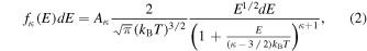
Examples of the relative ion abundances obtained from these ionization and recombination rates (assuming ionization equilibrium) are shown in Figure 2. Three examples are shown: the transition region O iv, the coronal Fe xiii, as well as the flare Fe xxi ion. The relative ion abundance is a function of κ through the dependence of both the ionization and recombination rate coefficients on κ (Dzifčáková & Dudík 2013), with the peaks of the relative ion abundances being lower and broader for low κ, as well as typically shifted to lower T for TR ions, and higher T for coronal and flare ions (see Dzifčáková & Dudík 2013, for details).
Figure 2. Behavior of the relative ion abundances with κ. Three examples are shown: O iv belonging to the transition region (left), Fe xiii, a coronal ion, and Fe xxi, which occurs during solar flares. Different colors denote different values of κ. Full lines correspond to the current version of KAPPA (and CHIANTI version 10), while the dashed lines show calculations from the previous version of KAPPA, corresponding to CHIANTI version 7.1.
Download figure:
Standard image High-resolution imageWe note that the majority of the ions are unaffected by the updated rates, but some minor changes can still occur for low values of κ with respect to the previous version of KAPPA (dashed lines in the left and right panel of Figure 2 for O iv and Fe xxi, respectively). We note, however, that these are typically within the precision of the ionization equilibrium calculations (cf. Heuer et al. 2021).
The update of the rates for Fe ions mostly affect the relative ion abundances of Fe viii and Fe ix (Section 4 of Dere et al. 2019). However, because at temperatures of around log(T [K]) ≈ 6, many overlapping Fe ions exist at similar temperatures, changes in the relative ion abundance of one Fe ion have knock-off effects on other ions. This is the case for Fe xiii (middle panel of Figure 2), where the peaks of the relative ion abundance for all κ are higher. Other subtle changes for low values of κ are also present, such as a change in the position of the peak for κ = 2 on the order of 10−2 of dex in log(T [K]).
3.2. Electron Excitation Rates
CHIANTI contains an extensive compilation of a huge number of atomic transitions, including Einstein coefficients Aji , Maxwellian-averaged collision strengths ϒij (nondimensionalized excitation rate coefficients; see, e.g., Phillips et al. 2008; Dudík et al. 2014b; Del Zanna & Mason 2018), as well as other quantities, such as wavelengths, energies of excited levels, proton excitation rates, and oscillator strengths. These values are being continuously updated, checked, rechecked (e.g., Dere et al. 2019; Del Zanna et al. 2015, 2021), as well as benchmarked against one another and also against spectroscopic observations (see, e.g., Del Zanna 2012a, 2012b). Since the publication of Paper I, there have been extensive changes to the atomic data contained in CHIANTI, requiring an almost complete recalculation of the excitation and deexcitation rates for κ-distributions in the KAPPA database. Note that for some ions the number of energy levels in CHIANTI increased by almost a half order of magnitude (e.g., Fe ix), accompanied by the requisite increase of level-to-level transitions. These updates of the KAPPA database represented a huge task, and we endeavored to complete it accordingly. We note, however, that this is an ongoing task due to the ongoing updates of the atomic data in CHIANTI itself. To avoid a possible mismatch between the Maxwellian calculations using the latest CHIANTI and the corresponding non-Maxwellian calculations for κ-distributions using KAPPA, a separate branch for the Maxwellian calculations was created in the KAPPA database and software (see Section 3.5).
For the non-Maxwellian κ-distributions, the cross sections σij or the nondimensionalized collision strengths Ωji are required to calculate the distribution-averaged collision strengths ϒij (T, κ) and ϒji (T, κ), see Dudík et al. (2014b) and references therein. Ωji is given by

where gi,j are the relative weights of levels i and j, whose excitation energies are Ei,j , a0 is the Bohr radius, σ are the excitation and deexcitation cross sections, and IH is the hydrogen ionization potential.
Because the calculations for Ωji are not usually publicly available and only the Maxwellian-averaged ϒji (T) are available in CHIANTI, Dzifčáková (2006) developed an approximate reverse-engineering method to obtain Ωji . The approximate method assumes a functional form for Ωji (see Section 3.3 of Dzifčáková et al. 2015),

where Cn and D are coefficients determined by the approximate method. The above equation needs to be supplemented with conditions for the behavior of Ω in the high-energy limit, which depend on the type of transition (for details, see Section 3.3 of Dzifčáková et al. 2015, and references therein).
The approximate method was tested with respect to calculations of ϒij (T, κ) using direct integration from Ω by Dzifčáková & Mason (2008) as well as Dzifčáková et al. (2015), where it was shown that the accuracy of ϒij (T, κ) obtained by the approximate method is excellent, typically within 5–10%. We note that this precision is comparable with the precision of the atomic data calculations themselves; see, e.g., Section 3 of Yu et al. (2018) as well as Heuer et al. (2021).
In the KAPPA database, ϒij
(T, κ) for each value of κ, including Maxwellian, are scaled using a factor  , while ϒji
(T, κ) are not scaled. Both are saved as IDL save files and also as machine-readable .ups and .dwns files, with separate files for each value of κ.
, while ϒji
(T, κ) are not scaled. Both are saved as IDL save files and also as machine-readable .ups and .dwns files, with separate files for each value of κ.
3.3. Two-ion Model
CHIANTI version 9 (Dere et al. 2019) introduced the two-ion model for calculating the level populations and satellite line intensities. Doubly excited states are mainly formed by the inner-shell excitation of ions in lower ionization states as well as by dielectronic capture of free electrons by ions in the higher-ionization states. These ions in the exitation-autoionization state can autoionize to produce an ion in the higher-ionization state, or are stabilized by a radiative transition to some excited level of an ion in a lower ionization state (see, e.g., Phillips et al. 2008; Del Zanna & Mason 2018). To calculate the population of the autoionizing state, it is necessary to solve the level populations for both ions simultaneously. In addition to the exception of transitions between bound levels for each of the ions, the rates for the autoionization levels also need to be included. This also allows including density effects on the satellite line intensities.
The autoionization rates Aauto are calculated in a similar way as for the bound levels. The effective collision strengths for κ-distributions are stored in .ups and .dwns files, together with the distribution-averaged collision strengths ϒji (T, κ) and ϒji (T, κ) for the bound levels.
The rate coefficients for dielectronic capture  from an ion in a higher-ionization state with an excited level k to a doubly excited state s of an ion in a lower ionization state for κ-distributions is given by Dzifčáková (1992),
where Ek and Es are the energies of states k and s, and gk and gs are their statistical weights.
The dielectronic satellite lines formed by radiative decays following dielectronic capture of free electrons into autoionizing levels are calculated using the level populations from the two-ion model. The calculation of satellite line intensities for κ-distributions follows the current CHIANTI implementation (see Dere et al. 2019) and the same method as in Paper I (see Section 3.5 therein).
3.4. Level-resolved Ionization and Recombination Rates
The current CHIANTI version 10 also contains level-resolved ionization and radiative recombination rates, i.e., ionization from and recombination to upper excited levels. These processes influence the relative-level populations and thus the line intensities. We included the level-resolved radiative recombination rates using the approximation of a power-law cross section, which is the same as for the total radiative recombination rate (see Section 3.3 of Dzifčáková and Dudík 2013). An alternative option is to use the Maxwellian decomposition method of Hahn & Savin (2015), where the sum of Maxwellians is first used to approximate κ-distributions (fκ (T) = ∑(ai fMaxw(bi T)), and a corresponding linear combination of Maxwellian rate coefficients is in turn used to calculate the rate coefficient for the κ-distribution.
Comparisons of level-resolved radiative recombination rates calculated using both methods are shown in Figure 3. The differences between these methods are small, as they reach about 2.5% for κ = 2, and are below 1% for κ ≥ 3.
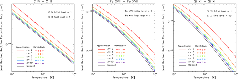
Figure 3. Comparison of the level-resolved radiative recombination rate calculated using our approximations (full lines) with the approximation of Hahn & Savin (2015; diamonds) for the transition from ground-level 1s2 2s2 S0.5 of C iv to ground-level 2s2 1 S0 of C iii (left), from the initial-level 2p5 2 P0.5 of Fe xviii to ground-level 2p6 1 S0 of Fe xvii, and from ground-level 1s2 2s2 2 S0.5 of Si xii to level 2p 3d3 D3 of Si xi. Individual colors represent different values of κ.
Download figure:
Standard image High-resolution imageSince version 9 of CHIANTI, level-resolved ionization rates are available for the Fe xvii–Fe xxii ions. However, no corresponding ionization cross sections are available (tabulated) for these ions. Therefore we used the method of Hahn & Savin (2015) to calculate the level-resolved ionization rates for κ-distributions. However, the Maxwellian level-resolved ionization rates are available in CHIANTI only for a relatively narrow temperature range, spanning only about one order. The method of Hahn & Savin (2015) requires ionization rates that cover at least about three orders of magnitude in temperature. Therefore extrapolations to both lower and higher temperatures had to be employed. We assumed that for the lower temperatures, the ionization rate Cioniz behaves like Cioniz ∼aebT , similarly to the extrapolation done by CHIANTI. For higher temperatures, we assumed that the Cioniz behaves as T−1/2 E1(EI/kB T), where EI is the ionization potential and E1 is the exponential integral of the first order. This type of behavior of the ionization rates with temperature can be expected; see, for example, Arnaud & Rothenflug (1985). Of course, different types of the extrapolations of ionization rates can lead to different extrapolated rates. Therefore we compared the Maxwellian ionization rates calculated by these extrapolations with the rates calculated by the extrapolation used in CHIANTI for lower temperatures (see Figure 4). The differences in the high-temperature ionization rates can be about a factor of 2 for the highest temperatures required by the Hahn & Savin (2015) method. However, due to relatively small multiplication factors ai in the Hahn & Savin (2015) approximations for high temperatures, these differences of the rate for κ-distributions decrease to about 25% at the highest temperature required. For the temperature corresponding to the maximum relative ion abundance, the differences can be on the order of 10%. Finally, the level-resolved ionization rates calculated by our extrapolation are shown in Figure 5 for different values of κ.
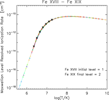
Figure 4. Extrapolation of the level-resolved ionization rate from the ground level of Fe xviii to level 2s2 2p4 3 P0 of Fe xix. Black points correspond to the rates tabulated in CHIANTI, while colored points denote temperatures for which Maxwellian rates are required to calculate the rates for κ-distributions using the Hahn & Savin (2015) approximation.
Download figure:
Standard image High-resolution image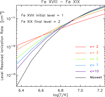
Figure 5. Ionization rates from the ground level of Fe xviii to level 2s2 2p4 3 P0 of Fe xix for different κ-distributions calculated by Hahn & Savin (2015). Individual colors represent the value of κ.
Download figure:
Standard image High-resolution image3.5. List of Routines in the KAPPA Software. Calculations for the Maxwellian and κ-distributions
As the CHIANTI database is being continuously updated, the possibility exists that the latest data available in CHIANTI will not be immediately translated into the data sets within the KAPPA database. For this reason, the users are advised to check whether the data sets are the same. To avoid possible problems and to facilitate consistent calculations once the data in the KAPPA database are updated, we created a separate Maxwellian branch within the KAPPA database, with the files containing the requisite atomic data for Maxwellian calculations being also retained in the databse. The Maxwellian branch of the software is characterized by the suffix _m.pro of the individual IDL routines, while the suffix _k.pro is used for κ-distributions. The latter always requires a value of κ as the first input. For example, the emiss_calc_m.pro and emiss_calc_k.pro routines are the equivalents of the CHIANTI emiss_calc.pro routine, which calculates the synthetic  (see Equation (6)) quantities for a particular ion.
A list of routines within the current version of the KAPPA database, together with the description of their function, is given in Table 1.
Table 1. List of Routines within the KAPPA Package Together with the Description of their Purpose
| Routine Name | Function |
|---|---|
| kappa.pro | interactive widget for calculating synthetic spectra, based on ch_ss.pro |
| ch_synthetic_k.pro | calculates line intensities as a function of κ, Ne, and T |
| ch_synthetic_m.pro | calculates line intensities as a function Ne and T for Maxwellian distributions and for the same atomic data |
| as for κ-distributions | |
| ch_load_ion_rates_k.pro | returns rates of a single ion for κ-distributions |
| ch_load_ion_rates_m.pro | returns Maxwellian rates of a single ion from the KAPPA database |
| ch_load_ion_2rates_k.pro | combines Kappa rates for two neighboring ions if the ion1 model has autoionization rates |
| ch_load_ion_2rates_m.pro | combines Maxwellian rates for two neighboring ions if the ion1 model has autoionization rates |
| ch_setup_ion_k.pro | reads the atomic parameters for κ-distributions into a structure that can be directly sent to the pop_solver_k |
| ch_setup_ion_m.pro | reads the atomic parameters from the KAPPA database into a structure that can be directly sent to the pop_solver_m |
| emiss_calc_k.pro | calculates hc/λ
 for the κ-distribution for the κ-distribution |
| emiss_calc_m.pro | calculates hc/λ
 for the Maxwellian distribution for the Maxwellian distribution |
| freebound_ion_k.pro | calculates the free-bound continuum arising from a single ion |
| freebound_k.pro | calculates the free-bound continuum |
| free–free_k.pro | free-free continuum interpolated from precalculated data |
| free–free_k_integral.pro | calculates the free-free continuum directly |
| get_contribution_k.pro | calculates contributions for κ-distributions |
| ion2filename_k.pro | converts the ion name into the name with a complete path to the KAPPA database |
| ion2filename_m.pro | converts the ion name into name with a complete path to the KAPPA database |
| ioniz_rate_k.pro | calculates the Kappa ionization rate for data from the KAPPA database |
| ioniz_rate_m.pro | calculates the Maxwellian ionization rate for data from the KAPPA database |
| isothermal_k.pro | calculates isothermal spectra for κ-distribution as a function of λ |
| isothermal_k.pro | calculates Maxwellian isothermal spectra for data from the KAPPA database as a function of of λ |
| kappa_dem.pro | calculates DEM for κ-distributions |
| k_diel_recomb.pro | calculates dielectronic recombination rates for κ-distributions |
| k_rad_recomb.pro | calculates radiative recombination rates for κ-distributions |
| k_tot_recomb.pro | calculates total recombination rates for κ-distributions |
| make_kappa_spec_k.pro | routine for calculating the synthetic spectra |
| plot_populations_k.pro | calculates and plots relative-level populations |
| pop_solver_k.pro | calculates the relative-level population for κ-distributions |
| pop_solver_m.pro | calculates the relative-level population for Maxwellian distributions |
| read_ff_k.pro | reads the precalculated free-free continuum as a function of Z and T |
| read_ioneq_k.pro | reads a CHIANTI format ionization equilibrium (ioneq) file for κ-distributions |
| read_ionrec_k.pro | reads ionization and recombination total population rates |
| read_kappa_ups.pro | reads Kappa upsilons and downsilons from the KAPPA database |
| read_mxw_ups.pro | reads Maxwellian upsilons and downsilons from the KAPPA database |
| read_rrlvl_k.pro | reads level-resolved recombination population rates for the κ-distribution |
| read_trans.pro | reads transition parameters for the κ-distribution |
| read_rate_ioniz_k.pro | reads the total ionization rates |
| read_rate_recomb_k.pro | reads the total recombination rates |
| ups_kappa.pro | converts the nuclear charge and charge state of an ion into the Kappa file name with the full path to the KAPPA database |
| ups_kappa_interp_str.pro | interpolates the ϒij (T, κ) and ϒji (T, κ) for the required temperature(s) |
| ups_mxw.pro | returns ϒij (T) for the Maxwellian distribution and temperature(s) |
| ups_mxw_interp_str.pro | interpolates Maxwellian upsilons for the required temperature(s) |
| zion2filename_k.pro | converts the nuclear charge and charge state of the ion into the file name with the full path to the KAPPA database |
| zion2filename_m.pro | converts the nuclear charge and charge state of the ion into the file name with the full path to the KAPPA database |
Download table as: ASCIITypeset image
4. Examples of Applications: Diagnostics of Plasma Properties
We now proceed to show examples of applications of the calculations using the KAPPA database. In doing so, we focus on the diagnostics of plasma parameters, such as Ne, T, and κ. Many of these methods were developed previously by Dzifčáková & Kulinová (2010), Mackovjak et al. (2013), Dudík et al. (2014b, 2015), Polito et al. (2016), Dzifčáková et al. (2018), and Lörinčík et al. (2020). In addition, the influence of κ on the DEM κ (T) was studied by Mackovjak et al. (2014), Dudík et al. (2015), and Lörinčík et al. (2020), who found that the peaks of the DEM κ (T) are typically shifted to higher T, although changes in the slope of the DEM can also occur with κ.
4.1. Electron Densities
The measurement of electron densities is often a prerequisite of diagnostics of κ (Dzifčáková & Kulinová 2010; Dudík et al. 2015; Lörinčík et al. 2020). The electron density can be determined using the ratio of two lines, involving at least one transition from a metastable level (Phillips et al. 2008; Del Zanna & Mason 2018). Here, we show four different line ratios used with current or previous instruments to measure Ne across the solar corona, TR, and flares. The TR O iv lines near 1400 Å (Dudík et al. 2014a) are observed by the Interface Region Imaging Spectrometer (IRIS; De Pontieu et al. 2014). Here, we present the O iv 1401.16/1404.81 Å line intensity ratio, which is sensitive to Ne in the range of ![$\mathrm{log}({N}_{{\rm{e}}}[{\mathrm{cm}}^{-3}])$](https://content.cld.iop.org/journals/0067-0049/257/2/62/revision1/apjsac2aa7ieqn8.gif) ≈ 9–12 (Figure 6, top right). The density-sensitive ratio is plotted for the Maxwellian distribution as well as for κ = 5 and 2 using black, green, and red colors, respectively. Because the O iv ion is formed in a range of temperatures depending on κ (see the left panel of Figure 2), we plot the ratio at the peak of the relative ion abundance (full lines) as well as the location in which the relative ion abundance drops down to 1% of its maximum (dotted and dashed lines for low and high T, respectively) in the same manner as used by Dudík et al. (2014b). It is seen that for κ = 2, the density-sensitive ratio is shifted to the left by about 0.3 dex in
≈ 9–12 (Figure 6, top right). The density-sensitive ratio is plotted for the Maxwellian distribution as well as for κ = 5 and 2 using black, green, and red colors, respectively. Because the O iv ion is formed in a range of temperatures depending on κ (see the left panel of Figure 2), we plot the ratio at the peak of the relative ion abundance (full lines) as well as the location in which the relative ion abundance drops down to 1% of its maximum (dotted and dashed lines for low and high T, respectively) in the same manner as used by Dudík et al. (2014b). It is seen that for κ = 2, the density-sensitive ratio is shifted to the left by about 0.3 dex in ![$\mathrm{log}({N}_{{\rm{e}}}[{\mathrm{cm}}^{-3}])$](https://content.cld.iop.org/journals/0067-0049/257/2/62/revision1/apjsac2aa7ieqn9.gif) (Figure 2) as a consequence of the behavior of the relative ion abundance (see Figure 2).
(Figure 2) as a consequence of the behavior of the relative ion abundance (see Figure 2).

Figure 6. Examples of line intensity ratios sensitive to the electron density. The black lines correspond to a Maxwellian, while the green and red lines stand for κ = 5 and 2, respectively. For each distribution, three curves are shown, those corresponding to the peak of the relative ion abundance (full lines), as well as where the ion has 1% of its peak (dotted and dashed lines). The line intensities are in units of phot cm−2 s−1 sr−1. These plots can be directly compared with those of Figures 6–7 of Dudík et al. (2014b) as well as Figure C.1 of Polito et al. (2016).
Download figure:
Standard image High-resolution imageFor the coronal ions, the changes in the density-sensitive line ratios with κ are much smaller, with κ = 2 yielding electron densities lower by only about 0.1 dex compared to the Maxwellian. Two examples of density-sensitive ratios are presented in Figure 6: that of the well-known and widely used Fe xii 186.89/192.39 Å and Fe xiii 203.83/202.04 Å (see, e.g., Young et al. 2009; Watanabe et al. 2009; Del Zanna 2011; Del Zanna et al. 2012; Del Zanna & Mason 2018; Dudík et al. 2014b, 2021). We note that our calculations for Fe xiii included the effect of photoexcitation by a 6000 K blackbody 0.01 R⊙ above the photosphere, which affects the Fe xiii line intensity ratio (see Young et al. 2009; Dudík et al. 2021). In addition, the Fe xii ratio is shown using the Fe xii 192.39 Å line rather than the 195.12 Å self-blend because the latter can be affected by opacity (Del Zanna et al. 2019).
The last example is the Fe xxi 145.73/128.75 Å ratio, which is used for measurements of electron densities in solar flares (Mason et al. 1979, 1984; Milligan et al. 2012; Del Zanna & Woods 2013; Dzifčáková et al. 2018). This ratio is sensitive to electron densities at ![$\mathrm{log}({N}_{{\rm{e}}}[{\mathrm{cm}}^{-3}])$](https://content.cld.iop.org/journals/0067-0049/257/2/62/revision1/apjsac2aa7ieqn10.gif) ≳ 11 (last panel of Figure 6). It is seen that for a given measured ratio, the electron densities are lower by about 0.15 dex if the electron distribution is κ = 2, compared to the Maxwellian.
≳ 11 (last panel of Figure 6). It is seen that for a given measured ratio, the electron densities are lower by about 0.15 dex if the electron distribution is κ = 2, compared to the Maxwellian.
4.2. Diagnostic Methods for κ
Another example of the usability of the KAPPA database is the calculation of synthetic spectra to search for emission lines that are sensitive to κ, and subsequently, to propose a new diagnostic method for κ-distributions. Figure 7 shows an example of a newly identified diagnostic ratio-ratio diagram. A ratio–ratio diagram consists of the dependence of one emission line ratio upon another emission line ratio, requiring use of at least three different emission lines (Dzifčáková & Kulinová 2010; Dudík et al. 2014b). Individual colored curves correspond to different values of κ. For our example, we considered a portion of the UV spectral range near 500 Å as well as 700 Å. This spectral range is currently observable by the SPICE instrument on board Solar Orbiter (Spice Consortium et al. 2020), with wavelengths near 500 Å observable in second order. At these wavelengths, O iii emission lines are found, whose ratios are sensitive to κ. For κ-distributions, these ratios change by a large factor compared to the Maxwellian. Depending on the temperature, the changes for κ = 2 can reach a factor of 2–4, with differences from the Maxwellian increasing for decreasing T (see Figure 7).

Figure 7. Example of a ratio-ratio diagram (involving two line intensity ratios) sensitive to both T and κ, involving the O iii lines together with their blends. The gray lines denote isotherms, with the values of log(T [K]) indicated.
Download figure:
Standard image High-resolution imageThe principal lines used here are the O iii 508.18 Å, 525.79 Å, and 702.90 Å. These lines are self-blends of several transitions, and in addition, they can be blended by O iii–O v transitions, whose importance changes depending on temperature, in some cases, creating a complex of oxygen lines consisting of many transitions. For instance, the O iii line at 508.18 Å contains five O iii transitions, with those at 507.39, 507.68, and 508.18 being important. In addition to this, there are four O iv and five O v blending transitions whose importance increases at higher temperatures. At log(T [K]) = 5, the dominant transition is already the O v 508.09 Å, with intensities of the 507.66, and 507.81, and 508.18 Å transitions being from a few tens up to 50% of the main transition. The other blending O iv transitions include the 508.11, 508.14, 507.18, and 508.02 Å ones, with each contributing a non-negligible amount.
The O iii line at 525.79 Å does have one self-blend at 525.80 Å. The O iii line at 702.84 Å is self-blended by two transitions at 702.90 and one at 702.34 Å, with an additional weak blend of O iv 702.34 Å. There are O v blends here as well, but their contribution at log(T [K]) = 5 is negligible. We note, however, that in the solar transition region, especially in case of constant pressure along a loop, the contribution of the O iii lines will dominate that of the higher-ionization stages of oxygen. This is because the electron density is higher at the lower formation temperature of O iii.
We note that at the low-T end of the ratio-ratio diagrams in Figure 7, the sensitivity to the κ-distributions is highest, reaching a factor of ≈4 for log(T [K]) = 4.5 (Figure 7). This sensitivity is much higher than the sensitivities obtained from coronal Fe lines in the extreme-UV (EUV; cf. Dudík et al. 2015; Lörinčík et al. 2020), which is at best a few dozen percent. This ratio-ratio diagram thus represents excellent previously unseen diagnostics opportunities for κ-distributions.
4.3. Coronal Forbidden Lines
As a final example, we show the full spectrum of Fe xiv in the range of 100–10,000 Å containing both the strong EUV lines longward of 200 Å as well as the green coronal forbidden line at 5303 Å (wavelength in air; see Del Zanna & DeLuca 2018). Previously, Dudík et al. (2014b) studied the signatures of κ-distributions in the Fe ix–Fe xiii spectra including their forbidden lines, and found that with decreasing κ, the intensities of the forbidden lines increase relative to the allowed EUV lines, sometimes by a factor of two, and in the case of the red Fe x 6376 Å line, by a factor of four. This could be a potential explanation for the relatively intense coronal forbidden lines, which are reported to extend up to about 2R⊙ by Habbal et al. (2013), as well as serve as a powerful diagnostics of κ-distributions if the forbidden lines are observed simultaneously together with the EUV lines.
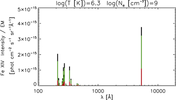
We now supplement the results of Dudík et al. (2014b) with the calculations for Fe xiv (Figure 8). The Fe xiv spectrum, calculated for a constant temperature of log(T [K]) = 6.3 and a constant coronal density of ![$\mathrm{log}({N}_{{\rm{e}}}[{\mathrm{cm}}^{-3}])$](https://content.cld.iop.org/journals/0067-0049/257/2/62/revision1/apjsac2aa7ieqn11.gif) = 9.0, is shown in Figure 8. With decreasing κ, the intensities of all lines decrease with respect to the Maxwellian. However, the forbidden 5303 Å line decreases less slowly than the allowed EUV lines, causing the Fe xiv 5304 Å/211.32 Å ratio to be enhanced by 73% for κ = 2 compared to the Maxwellian.
= 9.0, is shown in Figure 8. With decreasing κ, the intensities of all lines decrease with respect to the Maxwellian. However, the forbidden 5303 Å line decreases less slowly than the allowed EUV lines, causing the Fe xiv 5304 Å/211.32 Å ratio to be enhanced by 73% for κ = 2 compared to the Maxwellian.
Figure 8. Synthetic Fe xiv spectrum (photon units) from the EUV to the infrared portion of the spectrum. Individual colors represent the value of κ. The spectra are plotted for a constant log(T [K]) = 6.3 and constant ![$\mathrm{log}({N}_{{\rm{e}}}[{\mathrm{cm}}^{-3}])$](https://content.cld.iop.org/journals/0067-0049/257/2/62/revision1/apjsac2aa7ieqn12.gif) = 9.0. An emission measure of unity is assumed.
= 9.0. An emission measure of unity is assumed.
Download figure:
Standard image High-resolution image
We note that the above calculations are valid only for a constant log(T [K]) = 6.3 regardless of κ, which does not take into account the behavior of the relative ion abundances. Considering that the formation of Fe xiv is shifted to a higher temperature for κ = 2, one could calculate the κ = 2 spectrum instead for the temperature at which the relative ion abundance reaches its maximum for this value of κ; log  [K]) = 6.45. Comparing then this spectrum with the Maxwellian one calculated at log
  [K]) = 6.3, the Fe xiv 5304 Å / 211.3 Å ratio would still be enhanced by about 47% for κ = 2 compared to Maxwellian.
5. Summary
We have carried out an extensive update of the KAPPA database and software in order for it to be compatible with the latest version of CHIANTI, version 10. KAPPA was originally based on the CHIANTI database and software package. Since the publication of Paper I (Dzifčáková et al. 2015), CHIANTI underwent updates and upgrades through versions 8–10, including changes to the total ionization and recombination rates, extensive updates to the excitation rates, as well as the introduction of the two-ion models required for calculating the relative-level populations if the relative-level population is modified by ionization from and recombination to the excited levels. All of these changes are now reflected in the updated KAPPA database, 5 which makes it the state-of-art tool for calculating the synthetic optically thin spectra for the non-Maxwellian κ-distributions.
In addition, level-resolved ionization and recombination rates were obtained for when the ionization rates employ extrapolations based on assumptions of the behavior of the respective cross sections and the Maxwellian decomposition method of Hahn & Savin (2015). The accuracy of this method was tested with respect to the Maxwellian. We found a good precision, on the order of 10%, at temperatures at which the ion is formed. At temperatures higher by about one order of magnitude, the precision decreases to about 25%, which is still comparable to the uncertainties of the atomic calculations themselves, however.
Although we aim to keep the KAPPA database current, CHIANTI itself undergoes frequent updates to the atomic data stored therein. To avoid a future mismatch with the Maxwellian calculations done with the most recent CHIANTI, we created a separate branch for Maxwellian calculations in KAPPA itself, so that the calculations for the Maxwellian and κ-distributions can be done using the same atomic data sets. Should the need arise in the future, we encourage the users to request an update of the atomic data in the database.
Finally, we also provided examples of applications of the calculations of non-Maxwellian spectra with KAPPA, focusing on diagnostics of plasma parameters, including the search for novel observables and telltale signatures of κ-distributions. We found that the O iii lines that form at around 500 and 700 Å provide excellent diagnostics of κ. Some line intensity ratios change by a factor of up to 2–4 compared to Maxwellian, providing a sensitivity that is much higher than previously employed diagnostic methods based on iron lines. This illustrates that the KAPPA database is a powerful tool for calculations of the non-Maxwellian optically thin synthetic spectra.
The authors thank the referee for comments that helped improve the manuscript and for discussions regarding the nature of κ-distributions. The authors acknowledge support from the Grant Agency of the Czech Republic, grant Nos. 18-09072S and 20-07908S, as well as institutional support RVO:67985815 from the Czech Academy of Sciences. This work was partly supported by the project SOLARNET, which has received funding from the European Union Horizon 2020 research and innovation program under grant agreement No. 82413. CHIANTI is a collaborative project involving George Mason University, the University of Michigan (USA), the University of Cambridge (UK), and NASA Goddard Space Flight Center (USA). It is an unparalleled spectroscopic database, and the authors are very grateful for its existence and continued development.