


Abstract
We present the analysis of simultaneous Nuclear Spectroscopic Telescope Array (NuSTAR) and XMM-Newton data of eight Compton-thick active galactic nuclei (CT-AGN) candidates selected in the Swift-BAT 100 month catalog. This work is part of an ongoing effort to find and characterize all CT-AGN in the Local (z ≤ 0.05) Universe. We used two physically motivated models, MYTorus and borus02, to characterize the sources in the sample, finding five of them to be confirmed CT-AGN. These results represent an increase of ∼19% over the previous NuSTAR-confirmed, BAT-selected CT-AGN at z ≤ 0.05, bringing the total number to 32. This corresponds to an observed fraction of ∼8% of all AGN within this volume-limited sample, although it increases to 20% ± 5% when limiting the sample to z ≤ 0.01. Out of a sample of 48 CT-AGN candidates, selected using BAT and soft (0.3−10 keV) X-ray data, only 24 are confirmed as CT-AGN with the addition of the NuSTAR data. This highlights the importance of NuSTAR when classifying local obscured AGN. We also note that most of the sources in our full sample of 48 Seyfert 2 galaxies with NuSTAR data have significantly different lines of sight and average torus column densities, favoring a patchy torus scenario.
Export citation and abstract BibTeX RIS
1. Introduction
Active galactic nuclei (AGN) are accreting supermassive black holes in the central regions of galaxies. AGN are mainly believed to be responsible for the cosmic X-ray background (CXB): the diffuse X-ray emission from a few keV to a few hundred keV (e.g., Marshall et al. 1980; Comastri et al. 1995; Alexander et al. 2003; Gilli et al. 2007; Ueda et al. 2014). In particular, at the peak of the CXB (20−30 keV; Ajello et al. 2008), a significant fraction of the emission (∼15%–20%; Gilli et al. 2007; Ananna et al. 2019) is attributed to a large population of Compton-thick AGN (CT-AGN; sources with obscuring hydrogen column densities NH ≥ 1024 cm−2).
Nonetheless, in the nearby universe (z ≤ 0.1) the observed fraction of X-ray selected CT-AGN with respect to the total population is between 5% and 10% (e.g., Vasudevan et al. 2013; Ricci et al. 2015). This is much lower than the fractions predicted by most AGN population synthesis models, which require, to properly explain the CXB, values between 20% (Ueda et al. 2014) and 50% (Ananna et al. 2019). CT-AGN are difficult to detect in X-rays due to the large obscuration in their line of sight, which significantly suppress their intrinsic emission, particularly at energies below 10 keV. Taking this into account, observational bias estimates recover a fraction of CT-AGN in the Local Universe of at least ∼20% (e.g., Brightman & Nandra (2011); Ricci et al. (2015); and refer to Section 4.2 of Burlon et al. (2011) for details on underlying model assumptions).
Infrared surveys obtain high fractions of CT-AGN, based on X-ray non-detections of infrared-selected objects (e.g., Stern et al. 2014; Del Moro et al. 2016; Asmus et al. 2020). Without an X-ray characterization, however, it is difficult to estimate their contribution to the CXB. The same is true for any large optically or infrared-selected samples, which generally recover larger CT-AGN fractions, compared to X-ray studies. It is thus still necessary to reconcile the observed X-ray-selected CT-AGN fraction with CXB model predictions.
In order to successfully detect and characterize these heavily obscured sources, it is necessary to use hard (>10 keV) X-ray observatories, particularly in the Local Universe. 10 The Burst Alert Telescope (BAT) on board the Neil Gehrels Swift (hereafter Swift) observatory is an instrument designed to provide critical gamma-ray burst triggers as it surveys the whole sky (Barthelmy et al. 2005). The BAT is sensitive in the 15–150 keV range and, while searching for bursts and monitoring hard X-ray transients, it performs an all-sky hard X-ray survey. The Swift-BAT 105 month catalog (Oh et al. 2018) reports the results of this survey, including 1632 hard X-ray sources, ∼60% of which are non-beamed AGN in nearby (z < 0.2) galaxies. The BAT energy range is least biased against Compton-thick source detection, making the BAT catalog the ideal tool to perform a complete survey of CT-AGN.
The Clemson Compton-thick AGN (CCTAGN) 11 project has been targeting CT-AGN candidates within the BAT catalog, with the objective to find and characterize all obscured AGN in the Local (z < 0.05) Universe. In order to determine the true CT-AGN fraction, a volume-limited sample is needed, to overcome the bias against detection of the faintest sources. Indeed, almost 90% of CT-AGN in the BAT catalog have been discovered at z ≤ 0.05 (within ∼200 Mpc). In comparison, 90% of the population of unabsorbed and Compton-thin AGN falls within z ≤ 0.12 (Ricci et al. 2017), a factor 2.4 (in distance) higher.
The BAT catalog lists 417 AGN within z ≤ 0.05 (BAT 100 month catalog; A. Segreto et al. 2021 in preparation). In order to estimate their obscuring column densities, a soft X-ray follow-up (by i.e., Swift-XRT, Chandra, XMM-Newton, or Suzaku) is necessary. Using observations in the 0.3–10 keV range, previous works have classified 63 BAT sources within this volume as candidate CT-AGN (e.g., Ricci et al. 2015; Marchesi et al. 2017a, 2017b; R. Silver et al. 2021 in preparation). However, the uncertainties associated with most NH values are fairly large, due to the lack of high-quality data in the range bridging soft X-rays and BAT data (i.e., ≈7−15 keV).
The Nuclear Spectroscopic Telescope Array (hereafter NuSTAR; Harrison et al. 2013), observing in the range of 3–78 keV, provides a two orders of magnitude better sensitivity than previous telescopes at energies ≥ 10 keV. This allows one to characterize the properties of the AGN torus (i.e., average NH, inclination angle, covering factor), which mainly affect the reflected emission of the AGN; the so-called Compton hump, at energies ∼20–40 keV. The addition of NuSTAR data allows to break degeneracies between parameters, such as the photon index, the line-of-sight NH, and the reflected emission, thus improving our classification of the sources.
This work is a follow-up on that performed by Marchesi et al. (2018), which presented the analysis of the 38 candidate CT-AGN in the BAT 100 month catalog for which an archival NuSTAR observation existed (the largest sample of heavily obscured AGN analyzed with NuSTAR so far). The largest study before that contained 11 objects (Masini et al. 2016), and those before focused on single or few sources (e.g., Baloković et al. 2014; Puccetti et al. 2014; Annuar et al. 2015; Bauer et al.2015; Brightman et al. 2015; Koss et al. 2015; Rivers et al. 2015; Puccetti et al. 2016). This remains true for studies performed since (e.g., Zhao et al. 2019a, 2019b; Turner et al. 2020; Iwasawa et al. 2020). Such studies allow confirming or ruling out the Compton-thick nature of a candidate, bringing us closer to deriving the true fraction of CT-AGN in the local Universe.
In this work, we analyze eight additional CT-AGN candidates selected from the BAT catalog, for which we were awarded simultaneous NuSTAR and XMM-Newton data. These are part of the last 10 sources in the 63 CT-AGN candidate sample that were still missing NuSTAR data, bringing us closer to completing the classification of the full sample. In this work, we decouple the column density in the line-of-sight NH,los from the average column density of the torus, NH,av, as previous works have shown this strategy provides a better fit to the data (e.g., Marchesi et al. 2019). Furthermore, there is evidence suggesting the AGN torus is a clumpy medium (e.g., Risaliti et al. 2002; Elvis et al. 2004; Markowitz et al. 2014), in which these two values are not necessarily the same. Given this fact, we clarify that we refer to a CT-AGN as one that is Compton thick in the line of sight.
This work is organized as follows: In Section 2, we describe the sample selection and data reduction. In Section 3, we describe the X-ray analysis and the models used. In Section 4, we present our results and comment on the properties of our sources. Finally, in Sections 5 and 6, we present our discussion and conclusions, respectively.
2. Sample Selection and Data Reduction
The sample in this work is selected from CT-AGN candidates in the Palermo Swift-BAT 100 month catalog (A. Segreto et al. 2021, in preparation), detected in the Local (z < 0.05, D ≲ 200 Mpc) Universe. All sources in the sample have been previously analyzed using a combination of Swift-BAT and 2–10 keV data, with the results of best-fit models for their X-ray emission classifying them as CT-AGN candidates. However, their column density determination is compatible with NH < 1024 cm−2 within errors.
The classification of most sources as CT-AGN candidates was reported in Ricci et al. (2015), who fitted the sources using the physical torus model of Brightman & Nandra (2011). ESO 112-G006 is the only source in the sample that was instead analyzed by our group and the results of the preliminary analysis are unreported. In order to confirm (or rule out) their Compton-thick nature, we were awarded simultaneous NuSTAR and XMM-Newton observation time in Cycles 18 and 5, respectively, as part of a NuSTAR Large Program (NuSTAR proposal ID: 5197; PI: Marchesi). The details of these observations can be found in Table 1: overall, we were granted ∼500 ks of observations with NuSTAR and ∼200 ks with XMM-Newton (pre-data cleaning). We were also granted time to observe two other sources (NGC 3081 and ESO 565-G019), selected in the same way. These objects also have archival Chandra data and are analyzed in a companion paper (Traina et al. 2021).
Table 1. Source Observation Details
| Swift-BAT ID | Source Name | R.A. | Decl. | z | Telescope | Obs ID | Exp. Time | Obs Date |
|---|---|---|---|---|---|---|---|---|
| [deg (J2000)] | [deg (J2000)] | [ks] | ||||||
| (1) | (2) | (3) | (4) | (5) | (6) | (7) | (8) | (9) |
| J0030.9-5901 | ESO 112-G006 | 00 30 43.83 | −59 00 25.87 | 0.02885 | NuSTAR | 60561038002 | 56.0 | 2019 Nov 6 |
| XMM-Newton | 0852180101 | 19.1 | 2019 Nov 6 | |||||
| J0105.4-4211 | MCG 07-03-007 | 01 05 26.81 | −42 12 58.3 | 0.02988 | NuSTAR | 60561039002 | 54.7 | 2019 Nov 28 |
| XMM-Newton | 0852180201 | 18.4 | 2019 Nov 28 | |||||
| J0623.7-3213 | ESO 426-G002 | 06 23 46.42 | −32 12 59.51 | 0.02243 | NuSTAR | 60561040002 | 52.5 | 2019 Oct 9 |
| XMM-Newton | 0852180301 | 21.1 | 2019 Oct 9 | |||||
| J0656.2-4919 | LEDA 478026 | 06 56 11.95 | −49 19 50.0 | 0.04100 | NuSTAR | 60561041002 | 55.5 | 2020 Feb 23 |
| XMM-Newton | 0852180401 | 21.2 | 2020 Feb 23 | |||||
| J0807.9+3859 a | MRK 622 | 08 07 40.99 | +39 00 15.26 | 0.02335 | NuSTAR | 60561042002 | 54.2 | 2019 Sep 28 |
| XMM-Newton | 0138951401 | 6.9 | 2003 May 5 | |||||
| XMM-Newton | 0852180501 | 8.4 | 2019 Sep 28 | |||||
| J1800.0+6636 | NGC 6552 | 18 00 07.25 | +66 36 54.35 | 0.02656 | NuSTAR | 60561046002 | 48.6 | 2019 Aug 20 |
| XMM-Newton | 0112310801 | 7.4 | 2002 Oct 18 | |||||
| XMM-Newton | 0852180901 | 11.0 | 2019 Aug 20 | |||||
| J1253.3-4138 | ESO 323-G032 | 12 53 20.31 | −41 38 08.3 | 0.01600 | NuSTAR | 60561045004 | 50.2 | 2020 Feb 2 |
| XMM-Newton | 0852181201 | 18.3 | 2020 Feb 2 | |||||
| J2307.8+2242 | CGCG 475-040 | 23 07 48.86 | +22 42 37.0 | 0.03473 | NuSTAR | 60561047002 | 55.8 | 2019 Nov 29 |
| XMM-Newton | 0852181001 | 21.7 | 2019 Nov 30 |
Notes. (1) ID from the Palermo BAT 100 month Catalog (Marchesi et al. 2019). (2) Source name. (3) and (4) R.A. and decl. (J2000 Epoch). (5) Redshift. (6) Telescope used in the analysis. (7) Observation ID. (8) Exposure time, in kiloseconds. XMM-Newton values are reported for EPIC-PN, after cleaning for flares. (9) Observation date.
a ID from the 105 month catalog of Oh et al. (2018), as the source is not detected in the Palermo BAT catalog.Download table as: ASCIITypeset image
Table 1 also lists previous XMM-Newton observations taken from the archive for NGC 6552 and MRK 662, which we used to constrain variability either in the flux or the column density of the sources. Both sources had one additional observation, which we did not use due to high percentage of flaring time, which resulted in poor statistics. All sources have additional Swift-XRT observations, which due to low count statistics, do not allow constraining any possible NH variability.
The data retrieved for both NuSTAR focal plane modules (FPMA and FPMB; Harrison et al. 2013) were processed using the NuSTAR Data Analysis Software (NUSTARDAS) v1.8.0. The event data files were calibrated running the nupipeline task using the response file from the Calibration Database (CALDB) v20200612. With the nuproducts script, we generated both the source and background spectra, and the ancillary and response matrix files. For both focal planes, we used a circular source extraction region with a 75'' diameter (corresponding to ∼80% encircled energy fraction) centered on the target source (except for NGC 6552, for which a 50'' region was used due to high background counts). For the background, we used an annular extraction region (inner radius 100'', outer radius 160'') surrounding the source, excluding any resolved sources. The NuSTAR spectra have then been grouped with at least 20 counts per bin.
We reduced the XMM-Newton data using the SAS v18.0.0, cleaning for flaring periods and adopting standard procedures. The source spectra were extracted from a 30'' circular region (corresponding to ∼85% encircled energy fraction for EPIC-PN), while the background spectra were obtained from a circle that has a radius 45'' located near the source and is not contaminated by nearby objects. Each spectrum has been binned with at least 15 counts per bin.
We fitted our spectra using the XSPEC software (Arnaud 1996, in HEASOFT v6.26.1), taking into account the Galactic absorption measured by Kalberla et al. (2005). We used Anders & Grevesse (1989) cosmic abundances, fixed to the solar value, and the Verner et al. (1996) photoelectric absorption cross section. The luminosity distances are computed assuming a cosmology with H0 = 70 km s−1 Mpc−1, and ΩΛ = 0.73. We used χ2 as the fitting statistic.
3. X-Ray Spectral Analysis
In this section, we describe the different torus models used to fit the X-ray data of each galaxy. Results of the X-ray spectral analysis of each source can be found in Section 4. All sources have been fit in the range from 0.6 keV to 25−55 keV, with the higher energy limit depending on the point in which NuSTAR data is overtaken by the background. For every source, all models have been consistently applied to the same energy range.
We add a thermal emission component, mekal (Mewe et al.1985; Kaastra 1992; Liedahl et al. 1995), to all torus models, which is necessary to account for the soft excess below ∼1 keV. We report the best-fit parameters of this model in Section 4, but we note that the gaseous material surrounding the AGN and within the galaxy is likely to be multiphase and complex (see, e.g., Torres-Albà et al. 2018), and therefore the derived temperature values, kT, should not be taken as accurate estimates of the physical properties of the galaxy.
We also add an additional scattered component, to characterize the intrinsic power-law emission of the AGN that either leaks through the torus without interacting with it, or interacts with the material via elastic collisions. This component is set equal to the intrinsic power law, multiplied by a constant, Fs, that represents the fraction of scattered emission (typically of the order of few percent, or less).
Finally, we take into account the Galactic absorption via the inclusion of a photoelectric absorption (phabs) component to the models.
3.1. MYTorus in Coupled Configuration
The MYTorus model of Murphy & Yaqoob (2009) assumes an isotropic X-ray emission within a uniform, neutral (cold) torus. The half-opening angle of the torus is fixed to 60°.
The MYTorus model is decomposed into three different components: an absorbed line-of-sight emission, a reflected continuum, and a fluorescent line emission. These components are linked to each other with the same normalization, absorbing column density (the model yields the equatorial column density of the torus, NH,eq) and inclination angle θi. The inclination angle is measured from the axis of the torus, so that θi = 0° represents a face-on AGN, and θi = 90° an edge-on one.
The line-of-sight column density of the torus can be obtained from the equatorial value as

and the average torus column density is determined by the given configuration as NH,av = π/4 × NH,eq, and cannot be decoupled (i.e., fit separately) from the line-of-sight value.
Both the reflected continuum and line emission can be weighted via two additional constants, AS and AL, respectively. When left free to vary, these can account for differences in the actual geometry (compared to the specific model assumptions used in the original calculations) and time delays between direct, scattered, and fluorescent line photons.
In XSPEC, this model configuration is as follows:
where C is a cross-calibration constant between different instruments, or a cross-normalization constant between different observations.
3.2. MYTorus in Decoupled Configuration
The MYTorus model can also be used in decoupled configuration (Yaqoob 2012), so as to better represent the emission from a clumpy torus. While the model has the exact same assumptions, a better description of the data is possible when decoupling the line-of-sight emission from the reflection component. That is, NH,los and NH,av are not fixed to the same value, allowing the flexibility of having a particularly dense line of sight in a (still uniform) Compton-thin torus, or vice versa.
In this configuration, the line-of-sight inclination angle is always fixed to θi = 90°, and two reflection and line components are included, one with θi = 90° (forward scattering) and weighted with AS,L90 and one with θi = 0° (backward scattering) and weighted with AS,L0. Note that in this configuration θi is no longer a variable, although the ratio between AS,L0/AS,L90 can give a qualitative idea of which direction reflection predominantly comes from, and therefore of the relative orientation of the AGN. 12
In XSPEC this model configuration is as follows:
We fix AS,90 = AL,90 and AS,0 = AL,0. In the default MYTorus decoupled scenario, we freeze all these constants to unity. However, we also include the results of thawing them both, which in some cases improves fit quality. We call this third model MYTorus decoupled free.
3.3. BORUS02
The other model used in this work is borus02 (Baloković et al. 2018). This model also assumes a uniform torus, but the opening angle is not fixed, and different geometries can be considered through the covering factor, CF parameter (CF ∈ [0.1, 1]). The model only includes a reflection component, which contains both the continuum and lines, meaning that an absorbed line-of-sight component must be added.
By default, we use this model in a decoupled configuration, with NH,los and NH,av set to vary independently. An advantage of this model, aside from including a variable covering factor, is that θi (with θi ∈ [18°–87°]) can still be fitted in a decoupled configuration. borus02 also includes a high-energy cutoff and iron abundance as free parameters, although we freeze them to 500 keV (consistent with the default setting in MYTorus) and 1, respectively, due to our inability to constrain them. We note that some works estimate lower (∼200 keV) high-energy cutoffs (e.g., Ricci et al. 2017; Ananna et al. 2020). However, the most recent work of Baloković et al. (2020) focuses on the local obscured AGN population (i.e., more similar to our sample properties) and places the average cutoff at ∼300 keV. They also show that systematic uncertainties allow for a relatively wide range, which marginally includes 500 keV. Note, also, that with NuSTAR data reaching up to 25–55 keV energies, the different high-energy cutoff values do not impact our results. CGCG 475-040 is the exception to this rule, as it required a very low high-energy cutoff to adequately fit the data.
In XSPEC this model configuration is as follows:
where zphabs and cabs are the photoelectric absorption and Compton scattering, respectively, applied to the line-of-sight component.
4. Results
In this section we describe the results obtained via X-ray spectral fitting, using simultaneous XMM-Newton and NuSTAR data, and compare them to previous determinations (when available). We note that the MYTorus coupled fits to the data are generally worse, statistically speaking, and often in disagreement with the results of other models (with the two exceptions justified in the text). This is a result of not allowing the NH,los and NH,av to vary independently, which may yield an averaged-out value. Due to this fact, the discussion of the fitting results for each source does not take the MYTorus coupled model into consideration. We will further discuss the validity of this model in Section 5.
An example table showing the best-fit parameters for ESO 112-G006, Table 2, is presented in the text. Tables for the rest of sources can be found in Appendix A. The tables also give our estimation of flux (observed) and luminosity (intrinsic) derived using each best-fit model and the cflux and clumin XSPEC convolution components. The equivalent width of the iron Kα line (EW) is computed as described in Marchesi et al. (2018). All errors reported are at a 90% confidence level unless otherwise stated.
Table 2. X-Ray Fitting Results of ESO 112-G006
| Model | MYTorus | MYTorus | MYTorus | borus |
|---|---|---|---|---|
| (Coupled) | (Decoupled) | (Decoupled Free) | ||
| red χ2 | 1.08 | 1.27 | 1.08 | 1.02 |
| χ2/dof | 276.61/256 | 325.42/256 | 274.29/254 | 260.37/254 |
| kT |

|

|

|

|
| Γ |

|

|

|

|
| NH,los |

|

|

|

|
| NH,eq |

| ⋯ | ⋯ | ⋯ |
| NH,av | ⋯ |

|

|

|
| AS90 | ⋯ | 1 a |

| ⋯ |
| AS0 | ⋯ | 1 a | 0 a | ⋯ |
| CF | ⋯ | ⋯ | ⋯ |

|
| cos(θi ) |

| ⋯ | ⋯ |

|
| Fs (10−3) |

| 0 a |

|

|
| Norm (10−4) |

|

|

|

|
| EW [keV] |

|

|

| ⋯ |
| Flux (2−10 keV) [10−13] |

|

|

|

|
| Flux (10−40 keV) [10−12] |

|

|

|

|
| Lintr (2–10 keV) [1042] |

|

|

|

|
| Lintr (15–55 keV) [1043] |

|

|

|

|
| Counts | 7053 | |||
Notes.
red χ2: reduced χ2.
χ2/dof: χ2 over degrees of freedom.
kT: mekal model temperature, in units of keV.
Γ: power-law photon index. NH,los: line-of-sight torus hydrogen column density, in units of 1024 cm−2.
NH,av: equatorial torus hydrogen column density, in units of 1024 cm−2.
NH,av: average torus hydrogen column density, in units of 1024 cm−2.
AS90: constant associated with the reflection component, edge-on. AS0: constant associated with the reflection component, face-on.
CF: covering factor of the torus, ∈[0.1–1].
cos(θi ): cosine of the inclination angle. cos(θi ) = 1 represents a face-on scenario.
Fs : fraction of scattered continuum. Norm: normalization of the AGN emission. EW: equivalent width of the neutral iron K-alpha line.
Fluxes (observed) are given in units of erg s−1 cm−2.
Luminosities (intrinsic) are given in units of erg s−1.
Total net counts used for fitting: XMM-Newton in the 0.6−9 keV band, and NuSTAR from 3 to 25–55 keV (depending on the source. See the full range for each source in the plots shown in the Appendix).
a Variable fixed to the respective value. Unreported upper/lower limits for any variable represent the inability of the model to provide them (i.e., the parameter is compatible within a 90% error with the model hard limits).Download table as: ASCIITypeset image
Likewise, we show plots of the MYTorus decoupled free and borus02 fits to the data for ESO 112-G006 in Figure 1, and the rest of figures (Figures 5–13) can be found in Appendix B.

Figure 1. X-ray spectral fitting (unfolded) of ESO 112-G006 using MYTorus the in decoupled free configuration (left) and borus02 (right). In both plots, XMM-Newton and NuSTAR data are plotted in red and blue crosses, respectively. The best-fit convolution model is shown as a solid, green line. The different components are shown as black lines: line-of-sight emission (solid), reflected emission (dashed in borus02. For MYTorus, the 90° reflection is shown as a dashed line, and the 0° reflection as a dotted line), scattered emission (dashed–dotted-dot–dot) and soft thermal emission (dashed dotted). Note that this particular source does not show any 0° reflection in the MYTorus model.
Download figure:
Standard image High-resolution image4.1. ESO 112-G006
This source was first reported as a CT-AGN candidate by Ricci et al. (2015), who obtained a value of log  based on XMM-Newton and Swift-BAT observations. There are no optical classifications on its activity type, but its optical spectrum (Jones et al. 2009) does not present any broad emission lines. Results of the fitting can be found in Table 2.
This source is well fitted by all models except for MYTorus decoupled. Note that, generally, MYTorus decoupled provides a better fit than the coupled version. This is likely because, for this particular source, there is no contribution coming from face-on reflection, and the mentioned model assumes AS0 = AS90 = 1. Indeed, MYTorus decoupled free is a better fit, showing a clear predominance of forward reflection, which agrees with the borus02 inclination angle being large (cos(θi ) <0.3).
All models are in agreement that this source is observed through a Compton-thin line-of-sight (NH,los = 0.47−0.67 ×1024 cm−2), while the average torus material is denser, and even Compton -thick (NH,av = 0.71–2.42 × 1024 cm−2). According to the borus02 best-fit model, this Compton-thick torus would be geometrically thin, with a relatively small covering factor ( ). The photon index lies in the range Γ =1.40–1.83, when considering all the different models.
4.2. MCG 07-03-007
MCG 07-03-007
13
was first reported as a CT-AGN candidate by Ricci et al. (2015), who obtained a value of log  based on Swift-XRT and Swift-BAT observations. The source is optically classified as an Sy2 (Baumgartner et al. 2013). Results of the fitting can be found in Table 5.
All models are in good agreement for the description of the source. It is marginally Compton thin in the line-of-sight (NH,los = 0.73–0.97 × 1024 cm−2), with Γ ∼ 1.8 and a Compton-thick torus. The results of MYTorus decoupled free have larger uncertainties, likely due to the fact that the addition of two more parameters is not required by the fit. borus02 gives a best fit with a covering factor of 0.6, just barely intercepted by the line of sight.
4.3. ESO 426-G002
This source was selected as a candidate CT-AGN based on our own Swift-XRT and Swift-BAT analyses, which is unreported in any previous publications. Optically, it is classified as an Sy2 (Baumgartner et al. 2013). Results of the fitting can be found in Table 6.
This source is clearly best fit by MYTorus decoupled free and borus02, with remarkably similar results, which (except for the photon index) do not differ significantly from the MYTorus decoupled best-fit model. According to our analysis, this source is borderline Compton thick in the line of sight, and Compton thick in the average torus material (NH,los = 0.92–1.09 × 1024 cm−2, NH,av = 2.86–4.64 × 1024 cm−2). borus02 can constrain the covering factor and inclination angle with high accuracy thanks to the clear dominance of the reflection component. For this source, the dominance of forward reflection (according to MYTorus decoupled free) would lead us to believe that the source has a large inclination angle, but borus02 results place it at θi ∼ 30°. It could be that, given the large covering factor ( ), most of the reflection comes through the torus, which MYTorus interprets as 90° reflection, regardless of the actual direction.
4.4. LEDA 478026
This source was first reported as a CT-AGN candidate by Ricci et al. (2015), who obtained a value of log  based on Swift-XRT and Swift-BAT observations. Optically, it is classified as an Sy2 (Baumgartner et al. 2013). Results of the fitting can be found in Table 7.
For this source, MYTorus decoupled free and borus02 are in strong agreement, fitting it as Compton thick in the line-of-sight (NH,los ∼ 1.45 × 1024 cm−2), with a lower average torus column density (NH,av ∼ 0.33 × 1024 cm−2). With an estimated covering factor of only CF = 0.15, this source is likely to have a very patchy torus. In this scenario, the low covering factor should not be interpreted geometrically (i.e., like in a thin disk-like torus) but rather physically, meaning that the surrounding clouds obscure only a small fraction of the available volume.
Contrary to this, MYTorus decoupled gives a different estimation for all the significant parameters, with a harder photon index, Compton-thin line of sight and Compton-thick torus. However, the fit is statistically worse, and the MYTorus decoupled free results point toward a strong dominance of only forward reflection (agreeing with the borus02 edge-on viewing angle). This leads us to favor the former scenario, given how MYTorus decoupled is limited by forcing AS,L90 = AS,L0 = 1.
4.5. MRK 622
This source was first reported as a CT-AGN candidate by Ricci et al. (2015), who obtained a value of log  14
based on XMM-Newton and Swift-BAT observations. Optically, it is classified as an Sy2 (Véron-Cetty & Véron 2006). Results of the fitting can be found in Tables 8 and 9, the latter of which includes the second XMM-Newton observation, taken from the archive.
14
based on XMM-Newton and Swift-BAT observations. Optically, it is classified as an Sy2 (Véron-Cetty & Véron 2006). Results of the fitting can be found in Tables 8 and 9, the latter of which includes the second XMM-Newton observation, taken from the archive.
In the case of MRK 622, the MYTorus model does not show a statistical improvement when adding additional free parameters. All models place this source as having a Compton-thick torus (NH,av = 0.63–3.11 × 1024 cm−2), while having a much lower line-of-sight column density (NH,los = 0.15–0.29 ×1024 cm−2). There is a disagreement between the best-fit photon index value between the MYTorus model and the borus02 model, with the first set at  , and the second at
  . The determination of torus properties, such as covering factor and opening angle, is made difficult by the fact that the reflection component is subdominant with respect to the line of sight (hence, the unconstrained values). This is also likely to be the reason for MYTorus decoupled free to not show a statistical improvement of fit, as the added parameters model reflected emission.
When adding the archived data, we introduce a cross-normalization constant, C, and a different line-of-sight hydrogen column density, NH,los2, and leave both free to vary. The addition does not result in significant changes or incremented agreement between the different models. However, leaving NH,los2 free to vary results in a best-fit value of NH,los2 = 0.39–0.69 × 1024 cm−2, which is incompatible within the errors with the best-fit value for NH,los, for all models (see Figure 2). Therefore, we conclude that this source presents line-of-sight NH variability at different epochs.
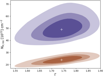
Figure 2. Confidence contours at 68%, 90%, and 95% levels, of photon index and line-of-sight hydrogen column density determinations, for the two XMM-Newton observations of MRK 622 (in blue, 2003 May 5, and in brown, 2019 September 28).
Download figure:
Standard image High-resolution image4.6. NGC 6552
This source was first reported as a CT-AGN candidate by Ricci et al. (2015), who obtained a value of log  based on XMM-Newton and Swift-BAT observations. Optically, it is classified as an Sy2 (Lin et al. 2012). Results of the fitting can be found in Tables 10 and 11, the latter of which includes the second XMM-Newton observation, taken from the archive.
All models are in agreement that this source has a Compton-thick line-of-sight (NH,los = 1.42–3.16 × 1024 cm−2) within a Compton-thin torus (NH,av = 0.30–0.55 × 1024 cm−2). The range of photon index values is relatively large (Γ = 1.53–2.11), although both MYTorus decoupled and decoupled free are compatible with the borus02 results within errors. The ratio between AS,90 and AS,0 suggests a predominance of forward reflection, which is compatible with the observation angle derived by borus02 , θi ∼ 75°.
When adding the archived observation, the data quality did not allow constraining NH,los2, and its value was compatible with that of NH,los. Therefore, the results presented in Table 11 have them fixed to be the same value. Both this and the fact that C is compatible with 1 makes us conclude that this source does not present variability between the two analyzed observations.
The addition of this second set of XMM-Newton data improves the overall agreement between the three models with good fitting statistics, and in particular between MYTorus decoupled free and borus02 . The qualitative description of the results would remain the same, with reduced uncertainty; NH,los = 1.42−2.56 ×1024 cm−2, NH,av = 0.34−0.63 × 1024 cm−2, and Γ = 1.57−1.84.
4.7. ESO 323-G023
This source was first reported as a CT-AGN candidate by Ricci et al. (2015), who obtained a value of log  based on Swift-XRT and Swift-BAT observations. It is optically classified as an Sy2 in Bird et al. (2007). This source has an additional XMM-Newton+NuSTAR joint observation (PI: Marchesi, Obs IDs: 0852180801 and 60561045002) that we do not use due to an error in the data taking. Results of the fitting can be found in Table 12.
All models fit this source with a slightly soft photon index (Γ ∼ 2.0) and a Compton-thick line-of-sight, NH,los = 1.12–3.21 ×1024 cm−2 (ignoring the MyTorus unconstrained result, as the statistics do not justify the addition of two extra free parameters). Also in agreement, they place the average torus column density to be slightly lower, NH,av = 0.49–1.79 × 1024 cm−2. Again, borus02 gives a best fit with a covering factor of 0.6, just barely intercepted by the line of sight.
4.8. CGCG 475-040
This source was first reported as a CT-AGN candidate by Ricci et al. (2015), who obtained a value of log  based on Swift-XRT and Swift-BAT observations. It is optically classified as an Sy2 in Parisi et al. (2014). Results of the fitting can be found in Table 13.
This source is best fit with a rather soft photon index, Γ = 1.9–2.60, and a large value of the average hydrogen column density when using the MYTorus model. The borus02 best fit of the NuSTAR+XMM-Newton data has two possible configurations fitting the data equally well: (1) a soft photon index, with a dense torus that has a large (∼90%) covering factor, and is viewed at a small inclination angle; (2) a photon index frozen to 1.8, with a very patchy torus (low average column density and covering factor, yet Compton thick in the line of sight). As both options have the same reduced χ2 we cannot say which model is superior.
To try and disentangle this degeneracy, we added Swift-BAT data to the spectrum,
15
as shown in Figure 13. We used borus02 to fit the data, as it is the only model providing an estimate for the torus covering factor, which we are interested in constraining within the two possible options mentioned above. With the addition of the BAT data, the best-fit model favors a scenario with a very dense torus of large covering factor, through which we observe the AGN through an underdense region (since  cm−2). Although the average torus density is capped at the maximum possible value (log NH,av = 25.5), we note that it is compatible with being only a factor ∼1.5 larger than that of the line of sight.
Interestingly, the BAT data can be adequately fit only when considering a cross-normalization factor between the NuSTAR+XMM-Newton data and the BAT data ( ). This implies our joint observation took place in a low-flux state of the source. It is also necessary to leave the high-energy cutoff free to vary, for which we obtain
  keV. This value, while being low, is not unprecedented (see the cutoff energy distribution of Swift-BAT sources; Ricci et al. 2017; Ananna et al. 2019). However, we caution that such a low high-energy cutoff can be spurious when NH is high and data quality is not exceptional (see the discussion in, e.g., Baloković et al.2020).
All models classify the source as Compton thick, with NH,los > 1024 cm−2. MYTorus decoupled free, despite having a Compton-thick best-fit value, is also compatible with a Compton-thin scenario within errors. However, we note that this model is statistically worse than MYTorus decoupled despite having two additional free parameters. This likely means MYTorus decoupled free has too many free parameters, which increases degeneracy and results in less reliable results.
5. Discussion
We classify a source as CT-AGN when its best-fit value for the line-of-sight hydrogen column density is NH,los ≥1024 cm−2. This corresponds to five out of the eight sources analyzed in this work (NGC 6552, ESO 426-G002, CGCG 475-040, ESO 323-G023, and LEDA 478026). Note that one of them, ESO 426-G002 is still compatible with having NH slightly below this threshold at 90% uncertainty. The other sources, although Compton thin, are still heavily obscured. Table 3 summarizes the best-fit borus02 parameters for the sample analyzed in this work.
Table 3. Best-fit borus02 Parameters for the Whole Sample
| Source | Γ | NH,los | NH,av | CF | cos θi |
|---|---|---|---|---|---|
| (1024 cm−2) | (1024 cm−2) | ||||
| ESO 112-G006 |

|

|

|

|

|
| MCG 07-03-007 |

|

|

|

|

|
| ESO 426-G002 |

|

|

|

|

|
| LEDA 478026 |

|

|

|

|

|
| MRK 622 |

|

|

|

|

|
| NGC 6552 |

|

|

|

|

|
| ESO 323-G032 |

|

|

|

|

|
| CGCG 475-040 |

|

|

|

|

|
Note. Parameters are as defined in Table 2. For sources with multiple observations, the best-fit values are taken from fitting them together. For MRK 622, which shows variable NH,los, the value listed is that of the joint NuSTAR and XMM-Newton observation, which has higher count statistics.
Download table as: ASCIITypeset image
5.1. Compton-thick Sources in the Local Universe
Ricci et al. (2015) provided a list of CT-AGN candidates in the 70 month BAT catalog, based on joint BAT and soft X-rays analysis (the best available data out of XMM-Newton, Chandra, Suzaku, Swift-XRT, and Advanced Satellitle for Cosmology and Astrophysics; ASCA). Out of a total of 55, 50 fall within z < 0.05. Based on the Palermo 100 catalog (Cusumano et al. 2015; A. Segreto et al. 2021, in preparation), other works (Marchesi et al. 2017a, 2017b; R. Silver et al. 2021 in preparation) have added to the list of possible CT-AGN within the BAT catalog. This comes to a total of 63 CT-AGN candidates at z ≤ 0.05.
Marchesi et al. (2018) analyzed 38 of these sources using NuSTAR data, which is key to disentangling the degeneracy between the photon index, Γ, the line-of-sight column density, NH,los, and the reflection component (which depends on the average column density, NH,av, inclination angle, and torus covering factor), and confirmed the Compton-thick nature of 17 them (originally 20 in Marchesi et al. (2018), but the reanalysis performed by Zhao et al. (2021) detailed in Section 5.2 reclassified three of them into Compton thin). Further works have brought the number of BAT-selected, confirmed CT-AGN at z ≤ 0.05, to a total of 29 (Koss et al. 2016; Oda et al. 2017; Georgantopoulos & Akylas 2019; Tanimoto et al. 2019; Kammoun et al. 2020; Zhao et al. 2020, 2021; Traina et al. 2021).
In this work, we report five additional NuSTAR-confirmed Compton-thick sources, bringing the current number to 32. This work thus represents an ∼19% increase of confirmed CT-AGN over the previous sample. The full list of NuSTAR-confirmed CT-AGN in the BAT catalog at z ≤ 0.05, along with the references to their analysis, can be found at our website. 16
According to the latest version of the Palermo BAT catalog (100 month catalog, A. Segreto et al. 2021, in preparation), there is a total of 414 BAT-detected AGN within z ≤ 0.05. We note that we are including galaxies lacking an optical classification as AGN (i.e., galaxy, galaxy in pair, galaxy in group, emission-line galaxy, and infrared galaxy), given how their bright emission at >15 keV is difficult to explain through other means. This implies that the number of confirmed CT-AGN within the volume-limited sample is still ∼8%, far from model predictions. The most recent estimate, that of Ananna et al. (2019), predicts, based on population synthesis models, a fraction of CT-AGN of ∼50%. Note, however, that this prediction is dependent on the flux of the sample considered. Our BAT sample is flux limited, and after applying the pertinent correction, should have a CT-AGN fraction between 27% and 38%, according to the model of Ananna et al. (2019)
We also note that our z < 0.05 is not necessarily complete. Indeed, we observe a significant trend with redshift of the CT-AGN fraction, which is higher (i.e., closer to predicted values) at lower redshifts. Figure 3 and Table 4 show the evolution of the observed CT-AGN fraction as a function of redshift, proving that indeed we can recover an ∼20% of CT-AGN in the lowest redshift bin. This value lies just below (when taking errors into account) the lower limit of the Ananna et al. (2019) estimations.
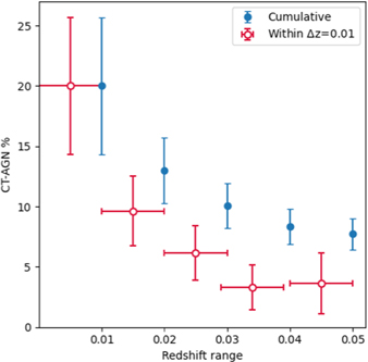
Figure 3. CT-AGN fraction within the BAT 100 month catalog (A. Segreto et al. 2021, in preparation) as a function of redshift. The red data represents the fraction within a a given redshift bin of 0.01, while the blue data points correspond to the cumulative value within <z. The computed fractions and total number of sources can be found in Table 4.
Download figure:
Standard image High-resolution imageTable 4. CT-AGN Fraction in the Local Universe
| Redshift | CT-AGN | Total AGN | CT-AGN% |
|---|---|---|---|
| z ≤ 0.01 | 10 | 50 | 20.0 ± 5.7 |
| z ≤ 0.02 | 20 | 154 | 13.0 ± 2.7 |
| z ≤ 0.03 | 27 | 268 | 10.1 ± 1.8 |
| z ≤ 0.04 | 30 | 359 | 8.4 ± 1.5 |
| z ≤ 0.05 | 32 | 414 | 7.7 ± 1.3 |
Note. Observed CT-AGN fraction in the Local Universe as a function of redshift. Total AGN include those in the BAT 100 month catalog within a given redshift bin. CT-AGN include those within the mentioned catalog, confirmed by NuSTAR as Compton thick. Errors are binomial.
Download table as: ASCIITypeset image
These results point to the sample being incomplete even at the lowest possible redshift, likely a result of the BAT flux limit. CT-AGN at higher redshift are likely too faint to be detected by BAT in the first place. We note that the errors listed in Table 4 and shown in Figure 3 are purely statistical, and do not account for any bias or incompleteness/obscuration corrections. Such predictions are nontrivial and are left for a future study.
In Figure 4, we show the sources with NuSTAR data targeted by our group as part of the CCTAGN project, our effort to characterize CT-AGN in the Local Universe. Out of the 48 objects analyzed by our group, 24 are found to be CT-AGN, which represents a success rate of ∼50%. This result showcases the need for NuSTAR data to confirm CT-AGN candidates, as all sources shown in the figure were compatible with being Compton thick based on soft X-rays and BAT data. It is possible that, without NuSTAR data and using simpler, phenomenological models, the selection based on BAT + soft X-ray data cannot properly distinguish between NH,los and NH,av, resulting in misclassifications (all Compton-thin sources in this work have a Compton-thick torus). We note that using the phenomenological models on the high-quality data we present here would result in the same effect. However, one can only apply the self-consistent, complex models (that allow disentanglement between NH,los and NH,av) in a meaningful way if NuSTAR data is available. That is because the reflection component dominates at ∼20 keV, a range in which no other satellite is sensitive enough.
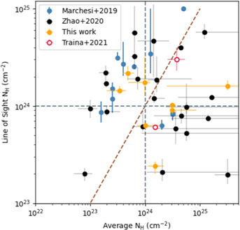
Figure 4. Line-of-sight hydrogen column density as a function of the average torus column density for the sources analyzed in this work (orange), in Marchesi et al. (2019) (blue), in Zhao et al. (2021) (black) and in Traina et al. (2021) (open symbols). All plotted results correspond to the best-fit borus02 model. The dashed vertical and horizontal lines mark the Compton-thick limit, while the diagonal line is a one-to one relation between NH,los and NH,av.
Download figure:
Standard image High-resolution imageThe mentioned, phenomenological models, which do not take into account the decoupling between NH,los and NH,av, are typically used in population synthesis models. The spectral shape of a source that is Compton thin in the line of sight but has a large NH,av might have a spectrum not so dissimilar from a source with a homogeneous Compton-thick torus, in which reflection is not taken into account in a self-consistent way. These sources, while not CT-AGN in the line of sight, might still contribute to the CXB in a relevant way. Therefore, we caution that our observed 20% ± 5% fraction of CT-AGN at z < 0.01 should be compared with the predictions of population synthesis models in a careful way.
5.2. Clumpy Torus Scenario
Based on our results, all eight sources except for ESO 323-G023 are incompatible, at 90% significance, with having the same line of sight and average torus column densities. Even for ESO 323-G023, the two values are compatible only at the very limits of their error range.
In Figure 4, we plot the sources analyzed by our group, comparing their line of sight and average torus column densities. Originally, Marchesi et al. (2018) analyzed the 38 sources in their sample using borus02 with the inclination angle frozen to θi = 90° to obtain an estimate of NH,av without leaving the parameter free to vary. Zhao et al. (2021) reanalyzed most of the sample (i.e., those sources with good-enough data quality) using the same methodology as described in this work. In Figure 4, we plot the sources as reanalyzed by Zhao et al. (2021) when available. 17 For those with insufficient data quality, we note that the determination of NH,av should be taken as a rough estimate. On the other hand, a comparison of NH,los for both analyses has shown little difference for most sources 18 Five additional sources are not included in the plot, due to having NH < 1023 cm−2 (2MASXJ10523297+1036205, RBS 1037, MCG-01-30-041, B2 1204+34, and ESO 244-30, Marchesi et al. 2019). These sources, all originally CT-AGN candidates, highlight even further the importance of using NuSTAR to estimate NH,los.
Figure 4 shows no strong correlation between one quantity and the other, and in fact, tend to fall far from the one-to-one relation. This is confirmed by our statistical analysis, which yields a Pearson correlation coefficient of ρ ≈ −0.02. 19 This means that sources that are Compton thick in the line of sight are no more likely to have a thicker torus than other sources. This result is in agreement with that found by Zhao et al. (2021), who analyzed a sample of ∼100 Compton-thin AGN in the Local Universe, which have high-quality NuSTAR and soft X-ray data, finding that NH,av is similar at different NH,los.
Furthermore, Figure 4 shows how most of the analyzed sources have significant differences between their estimated NH,los and NH,av values, which is a strong argument in favor of a patchy torus scenario. Observations both in the X-ray and in the near-IR band have already suggested that the structure of the obscuring material surrounding the supermassive black hole is, not surprisingly, more complex than a simple, homogeneous torus. Soft X-ray monitoring of AGN has shown variability in NH,los (e.g., Risaliti et al. 2002; Elvis et al. 2004; Markowitz et al. 2014). Infrared observations of AGN torus emission also support this scenario (Ramos Almeida et al. 2014). Despite this vision being largely accepted, there is still a small sample of sources for which NH variability has been confirmed, and other studies challenge this scenario after finding no variability in large samples (e.g., Laha et al. 2020, found no significant NH variability in 13/21 analyzed Sy2's).
In this work we also find NH,los variability for MRK 622 (in observations taken 16 yr apart), and we found none for NGC 6552 (in observations taken 17 yr apart). However, a complete analysis of column density variability and torus cloud distribution is beyond the scope of this work, and will be reported elsewhere. In order to draw stronger conclusions, we plan on targeting promising candidates in our sample (i.e., those with large NH,los/NH,av differences, or those with multiple observations), and analyze them with models based on clumpy torus distributions (e.g., UXClumpy; Buchner et al. 2019). A similar idea was proposed by Yaqoob et al. (2015). We leave this analysis for future work.
5.3. Agreement between Models
Generally, MYTorus and borus02 are in good agreement in their parameter estimation, particularly on their qualitative description of the source. That is, the models agree on Compton-thin versus Compton-thick classifications, both for NH,los and NH,av. They are also generally compatible in their photon index estimation (except for MRK 622 and ESO 112-G006), agreeing within errors for most of the sources.
This is not true when using MYTorus in a coupled configuration, as it tends to present strong disagreements with the photon index estimation, as well as systematically worse fits. Note, however, that the line-of-sight column density estimation is generally in agreement with that of the other models.
MYTorus decoupled and borus02 also agree in their qualitative description of the relative inclination of the source, with the ratio between AS,90 and AS,0 (showing predominance for forward or backward scattering) being consistent with the inclination angle and covering factor as estimated by borus02.
A detailed comparison of the MYTorus and borus02 performances can be found in Marchesi et al. (2019).
6. Conclusions
In this work we have analyzed eight CT-AGN candidates with simultaneous XMM-Newton and NuSTAR data, using the torus models MYTorus and borus02. For all of them, this is the first time their NuSTAR data is published. Our main conclusions are as follows:
- 1.Out of the eight analyzed sources, five are confirmed to be CT-AGN based on their XMM-Newton and NuSTAR data. This brings the total number of NuSTAR-confirmed CT-AGN in the BAT catalog at z ≤ 0.05 to 34.
- 2.Out of the 48 CT-AGN candidates analyzed as part of our project, 24 (∼50%) are confirmed CT-AGN with the addition of the NuSTAR data. This confirms the need for NuSTAR in order to fully ascertain the Compton-thick nature of obscured sources.
- 3.The percentage of confirmed CT-AGN within the BAT sample at z ≤ 0.05 is estimated to be ∼8% (34/417). Seven additional candidates remain to be analyzed, which were not included in this work due to the fact their NuSTAR data was not publicly available. If all sources turn out to be Compton thick, the total fraction of ∼10% will still be much lower than the Compton-thick fraction predicted by population synthesis models. This is likely a result of the suppression of the intrinsic CT-AGN emission even in the >15 keV band, as suggested by recent infrared studies (e.g., Yan et al. 2019; Carroll et al. 2021). It is also supported by the fact that we recover a CT-AGN fraction of 20% ± 5% within z < 0.01.
- 4.Most of the sources analyzed as part of our project are best fit with a line-of-sight column density, NH,los that differs, at ∼90% confidence, from their average torus column density, NH,av. This supports a patchy torus hypothesis.
- 5.We find no significant correlation between the average torus column density and the line-of-sight column density of our sample. This suggests that sources that are Compton thick in the line of sight are no more likely to have a thicker torus, on average, than those that are Compton thin.
- 6.We find that MRK 622 presented NH,los variability between observations at different epochs (17 yr apart) between NH,los ≈ 24 × 1022 cm−2 and NH,los ≈ 49 × 1022 cm−2.
N.T.A., M.A., R.S., and X.Z. acknowledge funding from NASA under contracts 80NSSC19K0531, 80NSSC20K0045 and, 80NSSC20K834. P.B. acknowledges financial support from the Czech Science Foundation project No. 19-05599Y. S.M. acknowledges funding from the INAF Progetti di Ricerca di Rilevante Interesse Nazionale (PRIN), Bando 2019 (project: "Piercing through the clouds: a multiwavelength study of obscured accretion in nearby supermassive black holes"). M.B. acknowledges support from the YCAA Prize Postdoctoral Fellowship. We thank Poshak Gandhi and Valentina La Parola for their helpful advice. The scientific results reported in this article are based on observations made by the X-ray observatories NuSTAR and XMM-Newton, and has made use of the NASA/IPAC Extragalactic Database (NED), which is operated by the Jet Propulsion Laboratory, California Institute of Technology under contract with NASA. We acknowledge the use of the software packages XMM-SAS and HEASoft.
Appendix A: X-Ray Fitting Results
Best fits results of all models used, for all sources in the sample.
Table 5. X-Ray Fitting Results of MCG 07-03-007
| Model | MYTorus | MYTorus | MYTorus | borus |
|---|---|---|---|---|
| (Coupled) | (Decoupled) | (Decoupled free) | ||
| red χ2 | 1.06 | 1.04 | 1.05 | 1.05 |
| χ2/dof | 239.45/227 | 237.17/227 | 236.25/225 | 236.98/225 |
| kT |

|

|

|

|
| Γ |

|

|

|

|
| NH,los |

|

|

|

|
| NH,eq |

| ⋯ | ⋯ | ⋯ |
| NH,av | ⋯ |

|

|

|
| A S90 | ⋯ | 1* |

| ⋯ |
| A S0 | ⋯ | 1* |

| ⋯ |
| CF (tor) | ⋯ | ⋯ | ⋯ |

|
| cos(obs) |

| ⋯ | ⋯ |

|
| Fs (10−3) |

|

|

|

|
| Norm (10−4) |

|

|

|

|
| EW [keV] |

|

|

| ⋯ |
| Flux (2−10 keV) [10−13] |

|

|

|

|
| Flux (10−40 keV) [10−12] |

|

|

|

|
| Lintr (2−10 keV) [1043] |

|

|

|

|
| Lintr (15−55 keV) [1043] |

|

|

|

|
| Counts | 5235 | |||
Note. Same as Table 2.
Download table as: ASCIITypeset image
Table 6. X-Ray Fitting Results of ESO 426-G002
| Model | MYTorus | MYTorus | MYTorus | borus02 |
|---|---|---|---|---|
| (Coupled) | (Decoupled) | (Decoupled Free) | ||
| red χ2 | 1.20 | 1.22 | 1.11 | 1.12 |
| χ2/dof | 409.12/341 | 414.95/341 | 366.53/339 | 380.25/339 |
| kT |

|

|

|

|
| Γ |

|

|

|

|
| NH,los |

|

|

|

|
| NH,eq |

| ⋯ | ⋯ | ⋯ |
| NH,av | ⋯ |

|

|

|
| AS90 | ⋯ | 1* |

| ⋯ |
| AS0 | ⋯ | 1* |

| ⋯ |
| CF | ⋯ | ⋯ | ⋯ |

|
| cos(θi ) |

| ⋯ | ⋯ |

|
| Fs (10−3) |

|

|

|

|
| Norm (10−3) |

|

|

|

|
| EW [keV] |

|

|

| ⋯ |
| Flux (2−10 keV) [10−13] |

|

|

|

|
| Flux (10−40 keV) [10−12] |

|

|

|

|
| Lintr(2-10 keV) [1043] |

|

|

|

|
| Lintr (15-55 keV) [1043] |

|

|

|

|
| Counts | 9492 | |||
Note. Same as Table 2.
Download table as: ASCIITypeset image
Table 7. X-Ray Fitting Results of LEDA 478026
| Model | MYTorus | MYTorus | MYTorus | borus |
|---|---|---|---|---|
| (Coupled) | (Decoupled) | (Decoupled free) | ||
| red χ2 | 0.90 | 0.98 | 0.89 | 0.90 |
| χ2/dof | 134.35/150 | 146.69/150 | 131.00/148 | 133.19/148 |
| kT |

|

|

|

|
| Γ |

|

|

|

|
| NH,los |

|

|

|

|
| NH,eq |

| ⋯ | ⋯ | ⋯ |
| NH,av | − |

|

|

|
| A S90 | ⋯ | 1* |

| ⋯ |
| A S0 | ⋯ | 1* |

| ⋯ |
| CF (tor) | ⋯ | ⋯ | ⋯ |

|
| cos(obs) |

| ⋯ | ⋯ |

|
| Fs (10−3) |

|

|

|

|
| Norm (10−3) |

|

|

|

|
| EW [keV] |

|

|

| ⋯ |
| Flux (2−10 keV) [10−13] |

|

|

|

|
| Flux (10−40 keV) [10−12] |

|

|

|

|
| Lintr (2-10 keV) [1043] |

|

|

|

|
| Lintr (15-55 keV) [1043] |

|

|

|

|
| Counts | 3761 | |||
Note. Same as Table 2.
Download table as: ASCIITypeset image
Table 8. X-Ray Fitting Results of MRK 622
| Model | MYTorus | MYTorus | MYTorus | borus02 |
|---|---|---|---|---|
| (Coupled) | (Decoupled) | (Decoupled free) | ||
| red χ2 | 1.26 | 1.25 | 1.26 | 1.22 |
| χ2/dof | 232.20/184 | 231.60/185 | 231.43/183 | 224.14/183 |
| kT |

|

|

|

|
| Γ |

|

|

|

|
| NH,los |

|

|

|

|
| NH,eq |

| ⋯ | ⋯ | ⋯ |
| NH,av | ⋯ |

|

|

|
| AS90 | ⋯ | 1* |

| ⋯ |
| AS0 | ⋯ | 1* |

| ⋯ |
| CF | ⋯ | − | ⋯ |

|
| cos(θi ) |

| − | ⋯ |

|
| Fs (10−2) |

|

|

|

|
| Norm (10−4) |

|

|

|

|
| EW [keV] |

|

|

| ... |
| Flux (2−10 keV) [10−13] |

|

|

|

|
| Flux (10−40 keV) [10−12] |

|

|

|

|
| Lintr (2−10 keV) [1042] |

|

|

|

|
| Lintr (15−55 keV) [1042] |

|

|

|

|
| Counts | 4938 | |||
Note. Same as Table 2.
Download table as: ASCIITypeset image
Table 9. X-Ray Fitting Results of Mrk 622—with Archival Data
| Model | MYTorus | MYTorus | MYTorus | borus02 |
|---|---|---|---|---|
| (Coupled) | (Decoupled) | (Decoupled free) | ||
| red χ2 | 1.38 | 1.23 | 1.25 | 1.20 |
| χ2/dof | 279.01/200 | 245.62/200 | 245.48/198 | 237.24/198 |
| kT |

|

|

|

|
| Γ |

|

|

| 1.74 
|
| NH,los |

|

|

| 0.24 
|
| NH,eq |

| ⋯ | ⋯ | ⋯ |
| NH,av | ⋯ |

| 1.99 
|

|
| AS90 | ⋯ | 1* |

| ⋯ |
| AS0 | ⋯ | 1* | 1.07 
| ⋯ |
| CF | ⋯ | ⋯ | ⋯ | 1.00 
|
| cos(θi ) |

| ⋯ | ⋯ | 0.84 
|
| Fs (10−2) | 2.19 
|

| 2.29 
|

|
| norm (10−4) |

|

|

|

|
| C |

|

|

|

|
| NH,los,2 | =NH,los |

|

|

|
| Counts | 6849 | |||
Note. Same as Table 2, with C: cross-normalization constant between observations and NH,los,2: line-of-sight torus hydrogen column density of the archived observation, in units of 1024 cm−2.
Download table as: ASCIITypeset image
Table 10. X-Ray Fitting Results of NGC 6552
| Model | MYTorus | MYTorus | MYTorus | borus02 |
|---|---|---|---|---|
| (Coupled) | (Decoupled) | (Decoupled free) | ||
| red χ2 | 1.47 | 1.12 | 1.10 | 1.12 |
| χ2/dof | 250.20/170 | 190.19/170 | 183.78/168 | 187.24/168 |
| kT |

|

|

|

|
| Γ |

|

|

|

|
| NH,los |

|

|

|

|
| NH,eq |

| ⋯ | ⋯ | ⋯ |
| NH,av | ⋯ |

|

|

|
| AS90 | ⋯ | 1* |

| ⋯ |
| AS0 | ⋯ | 1* |

| ⋯ |
| CF (tor) | ⋯ | ⋯ | ⋯ |

|
| cos(θi ) |

| ⋯ | ⋯ |

|
| F (10−4) | 0* |

|

|

|
| Norm (10−2) |

|

|

|

|
| EW [keV] |

|

|

| ⋯ |
| Flux (2−10 keV) [10−13] |

|

|

|

|
| Flux (10−40 keV) [10−12] |

|

|

|

|
| Lintr (2–10 keV) [1043] |

|

|

|

|
| Lintr (15–55 keV) [1043] |

|

|

|

|
| Counts | 6305 | |||
Note. Same as Table 2.
Download table as: ASCIITypeset image
Table 11. X-Ray Fitting Results of NGC 6552—with Archival Data
| Model | MYTorus | MYTorus | MYTorus | borus02 |
|---|---|---|---|---|
| (Coupled) | (Decoupled) | (Decoupled free) | ||
| red χ2 | 1.49 | 1.16 | 1.17 | 1.17 |
| χ2/dof | 288.66/194 | 225.69/194 | 223.85/192 | 225.31/192 |
| kT |

|

|

|

|
| Γ |

|

|

| 1.76 
|
| NH,los |

|

|

| 2.18 
|
| NH,eq |

| ⋯ | ⋯ | ⋯ |
| NH,av | ⋯ |

| 0.46 
|

|
| AS90 | ⋯ | 1* |

| ⋯ |
| AS0 | ⋯ | 1* | 0.43 
| ⋯ |
| CF | ⋯ | ⋯ | ⋯ | 0.40 
|
| cos(θi ) |

| ⋯ | ⋯ | 0.34 
|
| Fs (10−3) |

|

| 2.73 
|

|
| Norm (10−3) |

|

|

|

|
| C |

|

|

|

|
| NH,los,2 | =NH,los | =NH,los | =NH,los | =NH,los |
| Counts | 6849 | |||
Note. Same as Table 9.
Download table as: ASCIITypeset image
Table 12. X-Ray Fitting Results of ESO 323-G023
| Model | MYTorus | MYTorus | MYTorus | borus |
|---|---|---|---|---|
| (Coupled) | (Decoupled) | (Decoupled free) | ||
| red χ2 | 1.10 | 0.97 | 0.98 | 0.97 |
| χ2/dof | 132.21/122 | 118.58/122 | 117.09/120 | 116.9/120 |
| kT |

|

|

|

|
| Γ |

|

|

|

|
| NH,los |

|

|

|

|
| NH,eq |

| ⋯ | ⋯ | ⋯ |
| NH,av | − |

|

|

|
| A S90 | ⋯ | 1* |

| ⋯ |
| A S0 | ⋯ | 1* |

| ⋯ |
| CF (tor) | ⋯ | ⋯ | ⋯ |

|
| cos(obs) |

| ⋯ | ⋯ |

|
| Fs (10−4) |

|

|

|

|
| Norm (10−3) |

|

|

|

|
| EW [keV] |

|

|

| ⋯ |
| Flux (2−10 keV) [10−13] |

|

|

|

|
| Flux (10−40 keV) [10−12] |

|

|

|

|
| Lintr (2–10 keV) [1042] |

|

|

|

|
| Lintr (15–55 keV) [1042] |

| 1.56 
|

|

|
| Counts | 2566 | |||
Note. Same as Table 2.
Download table as: ASCIITypeset image
Table 13. X-Ray Fitting Results of CGCG 475-040
| Model | MYTorus | MYTorus | MYTorus | borus |
|---|---|---|---|---|
| (Coupled) | (Decoupled) | (Decoupled Free) | (with BAT) | |
| red χ2 | 1.18 | 1.12 | 1.13 | 1.07 |
| χ2/dof | 135.05/114 | 128.24/114 | 126.14/112 | 124.87/116 |
| kT |

|

|

|

|
| Γ |

|

|

|

|
| NH,los |

|

|

|

|
| NH,eq |

| ⋯ | ⋯ | ⋯ |
| NH,av | − |

|

|

|
| A S90 | ⋯ | 1* |

| ⋯ |
| A S0 | ⋯ | 1* |

| ⋯ |
| CF (tor) | ⋯ | ⋯ | ⋯ |

|
| cos(obs) |

| ⋯ | ⋯ |

|
| Fs (10−4) | 0* |

| 0* |

|
| Norm (10−3) |

|

|

|

|
| C | ⋯ | ⋯ | ⋯ |

|
| Ecut [keV] | ⋯ | ⋯ | ⋯ |

|
| EW [keV] |

|

|

| ⋯ |
| Flux (2−10 keV) [10−13] |

|

|

|

|
| Flux (10−40 keV) [10−12] |

|

|

|

|
| Lintr (2–10 keV) [1043] |

|

|

|

|
| Lintr (15–55 keV) [1043] |

|

|

|

|
| Counts | 2878 | |||
Note. Same as Table 2, with C: cross-normalization constant with BAT observation. Ecut: cutoff energy of the intrinsic power law.
Download table as: ASCIITypeset image
Appendix B: Figures
Best fits to the XMM and NuSTAR data of the MYTorus decoupled free and the borus02 models, for all sources in the sample.
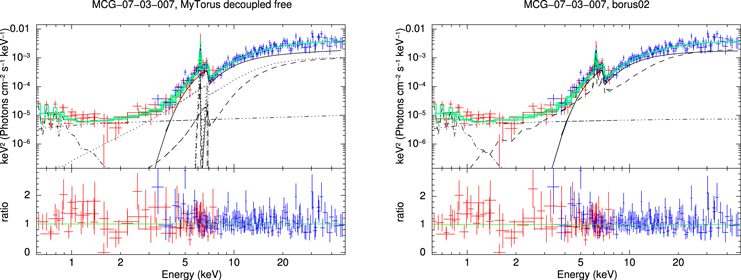
Figure 5. Same as Figure 1, for MCG 07-03-007.
Download figure:
Standard image High-resolution image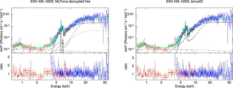
Figure 6. Same as Figure 1, for ESO 426-G002.
Download figure:
Standard image High-resolution image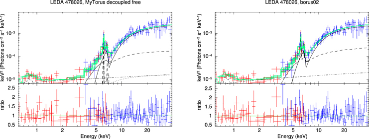
Figure 7. Same as Figure 1, for LEDA 478026.
Download figure:
Standard image High-resolution image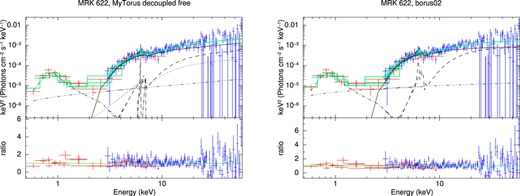
Figure 8. Same as Figure 1, for MRK 622.
Download figure:
Standard image High-resolution image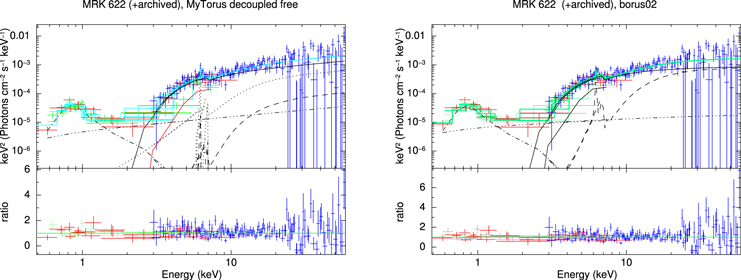
Figure 9. Same as Figure 1, for MRK 622, with the inclusion of a second XMM-Newton observation taken from the archive, plotted in gray crosses. For this source the two XMM-Newton observations were fitted with different NH,los, so we add the line-of-sight component for the second observation as a solid, red curve.
Download figure:
Standard image High-resolution image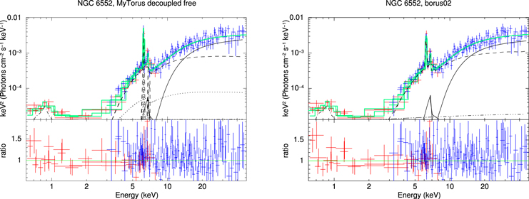
Figure 10. Same as Figure 1, for NGC 6552.
Download figure:
Standard image High-resolution image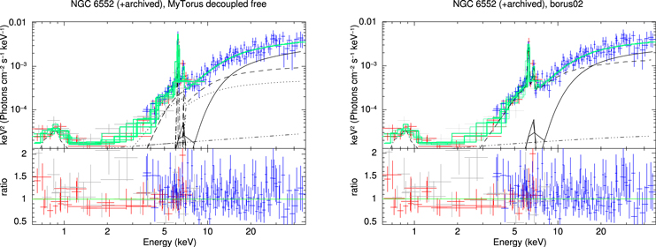
Figure 11. Same as Figure 1, for NGC 6552, with the inclusion of a second XMM-Newton observation taken from the archive, plotted in gray crosses.
Download figure:
Standard image High-resolution image
Figure 12. Same as Figure 10, for ESO 323-G032.
Download figure:
Standard image High-resolution image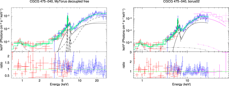
Figure 13. Same as Figure 10, for CGCG 475-040.
Download figure:
Standard image High-resolution image
Footnotes
- 10
- 11
- 12
We note that the normalization of both 0° and 90° scattering components is linked to that of the intrinsic continuum, and therefore it is necessary to leave both AS,0 and AS,90 free to vary.
- 13
We note that this source can be easily confused with UGC 0058, as it is mistakenly named MCG 07-03-007 or MGC 07-03-007 on occasion (without the minus sign in front), which in SIMBAD or NED redirects to the mentioned source. The correct position and redshift of the analyzed source can be found in Table 1.
- 14
No upper error available. Likewise, unreported upper/lower limits for any variable represent the inability of the used model to provide them (i.e., parameter is compatible within 90% error with the model hard limits).
- 15
We note that for no other source the addition of Swift-BAT data represented an improvement to the joint XMM-Newton+NuSTAR fit. Cutoff energy estimations for other sources in this work can be found in Ricci et al. (2017), who could not estimate Ecut for CGCG 475-040, possibly due to the mentioned parameter degeneracies.
- 16
https://science.clemson.edu/ctagn/. We encourage authors to contact us regarding any sources that might be missing.
- 17
- 18
Three sources were reclassified from Compton thick to Compton thin, and one from Compton thin to Compton thick. They had NH,los estimates close to the Compton-thick threshold.
- 19
ρ ≈ 1 or ρ ≈ −1 indicate strong linear correlation, or anticorrelation, respectively.