


Abstract
Several active galactic nuclei show correlated variations in the UV/optical range, with time delays increasing at longer wavelengths. Thermal reprocessing of the X-rays illuminating the accretion disk has been proposed as a viable explanation. In this scenario, the variable X-ray flux irradiating the accretion disk is partially reflected in X-rays and partially absorbed, thermalized, and reemitted with some delay by the accretion disk at longer wavelengths. We investigate this scenario assuming an X-ray pointlike source illuminating a standard Novikov–Thorne accretion disk around a rotating black hole. We consider all special and general relativistic effects to determine the incident X-ray flux on the disk and in propagating light from the source to the disk and to the observer. We also compute the disk reflection flux, taking into consideration the disk ionization. We investigate the dependence of the disk response function and time lags on various physical parameters, such as the black hole mass and spin; X-ray corona height, luminosity, and photon index; accretion rate; inclination; and inner/outer disk radii. We find it is important to consider relativistic effects and the disk ionization in estimating the disk response. We also find a strong nonlinearity between the X-ray luminosity and the disk response. We present an analytic function for the time-lag dependence on wavelength, which can be used to fit observed time-lag spectra. We also estimate the fraction of the reverberation signal with respect to the total flux, and we suggest possible explanations for the lack of X-ray–UV/optical correlated variations in a few sources.
Export citation and abstract BibTeX RIS
1. Introduction
According to the current paradigm, active galactic nuclei (AGN) are powered by the accretion of matter, in the form of a geometrically thin and optically thick disk, onto a central supermassive black hole (BH) of a mass MBH ∼ 106−9 M⊙. The viscous accretion disk (Pringle & Rees 1972; Novikov & Thorne 1973; Shakura & Sunyaev 1973) emits the bulk of its light in the UV/optical range and is responsible for most of the observed bolometric luminosity. AGN are known to be strong X-ray emitters as well. The X-rays are thought to be produced in the close vicinity of the BH, by hot electrons (∼109 K), located in a region known as the "X-ray corona." Thermal UV photons arising from the accretion disk will be Compton-upscattered off the energetic electrons in the X-ray corona, giving rise to the "primary emission" (e.g., Lightman & White 1988; Haardt 1993). The primary-emission spectrum is well described by a power law with a high-energy cutoff.
Part of the primary emission will be detected by the observer, and the other part will shine on the accretion disk. In the latter case, a fraction of the light will be reprocessed and emitted by the disk in X-rays (e.g., George & Fabian 1991; Matt et al. 1993). The other fraction will be absorbed by the disk, increasing its temperature, and be reemitted in the form of thermal UV/optical radiation. This will increase the UV/optical flux of the disk. In the event of a variable X-ray flux, the additional thermalized UV/optical flux will also be variable, with a time lag (with respect to the X-rays) increasing with wavelength. This mechanism is known as disk thermal reverberation (e.g., Cackett et al. 2007).
Various high-cadence monitoring campaigns, across the X-ray, UV, and optical bands, have been performed in the last few years, using space and ground-based telescopes (e.g., McHardy et al. 2014, 2018; Shappee et al. 2014; Cackett et al. 2018, 2020; Edelson et al. 2019; Hernández Santisteban et al. 2020). In general, the UV/optical variations are well correlated, with the optical variations being delayed with respect to the UV. This is in agreement with the hypothesis of disk thermal reverberation.
Recently we studied disk thermal reverberation in the case of NGC 5548 (Kammoun et al. 2019; hereafter KPD19). We computed the disk response to X-rays and the corresponding time lags, assuming a standard Novikov–Thorne (NT) accretion disk (Novikov & Thorne 1973) illuminated by a pointlike X-ray source located above the BH (known as a "lamp-post" geometry), as a simplified representation of an on-axis compact corona. The model took into account relativistic effects, and we computed the disk reflection, accounting for its ionization profile. We investigated the effects of the accretion rate and the height of the X-ray corona on the time lags between X-rays and the UV/optical band. We were able to fit the "lag versus wavelength" plot (this is known as a "time-lag spectrum") that Fausnaugh et al. (2016) previously estimated in NGC 5548, and we showed that the time-lag spectrum is in agreement with an NT disk accreting at a low rate, as long as the X-ray source is at a distance larger than 40 gravitational radii (Rg = GMBH/c2) above the BH.
In this work, we present the results from an extended study of disk thermal reverberation in the case of a lamp-post geometry. We compute the general relativity (GR) effects on the intrinsic X-ray spectrum of the corona, on the incident X-ray spectrum on the disk, and on the resulting X-ray reflection spectrum in more detail than KPD19 did. We show that there are significant differences in the disk response functions when we consider all the GR and disk ionization effects and when we use the approximations that have been usually assumed in the past. We compute and study the disk response for a wide range of values of model parameters—BH mass, accretion rate, corona height, energy spectral photon index, inclination angle, incident X-ray luminosity, and disk inner and outer radii. We compute time lags as a function of wavelength for the full parameter space, and we determine an analytic function for the time lags between X-rays and the UV/optical light curves that can be used to fit the observed time lags at least up to 5000 Å. We also compute the ratio of the thermally reverberating UV/optical disk flux to the underlying NT disk flux in various energy bands (the "reverberation fraction" hereafter). This ratio can be used to explain the nondetection of the variable UV/optical reverberating component in AGN, which is highly variable in X-rays. The paper is organized as follows.
In Section 2 we present the model setup, and we compare the model disk responses with the responses when using the approximations that have been frequently adopted in the past. In Section 3 we present the disk responses for a wide range of model parameter values. In Section 4 we discuss possible implications of our results, and in particular, we compute the time-lag spectra and we derive the analytic expression for the time lags as a function of wavelength. We also discuss the reverberation fraction for the parameter space that we consider. We conclude with a short summary of our results.
2. Model Setup
Similar to KPD19, we consider a Keplerian geometrically thin and optically thick accretion disk around a BH of mass MBH and accretion rate  in the Kerr metric.5
The disk temperature profile follows the NT prescription, with a color temperature correction factor of 2.4 (Ross et al. 1992). As a model for the corona, we assume a lamp-post geometry: the X-ray source is pointlike and is located at a height h above the BH, on its rotational axis.
in the Kerr metric.5
The disk temperature profile follows the NT prescription, with a color temperature correction factor of 2.4 (Ross et al. 1992). As a model for the corona, we assume a lamp-post geometry: the X-ray source is pointlike and is located at a height h above the BH, on its rotational axis.
In order to study disk thermal reverberation when the disk is illuminated by variable X-rays, we need to determine the disk response to an X-ray flash. We assume that the X-ray corona emits isotropically (in its rest frame) a power-law spectrum of the form  , where Γ is the spectral photon index (assumed to be constant). The flash lasts for Δt = 10 Tg (where Tg is the light travel time of the gravitational radius, Rg), and it has a top-hat shape (i.e., N(t) has a constant, nonzero value for 0 ≤ t ≤ 10 Tg, and then N(t) = 0 for t > 10 Tg). Since we use numerical computations, we cannot assume an ideal δ-function, but we approximate the X-ray flash with the top-hat function instead with a carefully chosen width. This width is small enough to avoid inaccuracies in our computations of the responses (especially for the response duration and average response time), and at the same time it is large enough to achieve reasonable computing times to get response functions that are smooth enough (i.e., without numerically caused oscillations). The flash duration of 10 Tg amounts to 5.7 × 10⁻³ days for a BH mass of 107 M⊙, thus being much shorter than the average response duration, which is usually measured in the order of days (i.e., shorter by more than two orders of magnitude). It is even shorter than the start time of the response (with the exception of low heights below ∼10 Rg and high inclinations above ∼60°). For more details we refer the reader to Figures 8, 10, and 12 in Appendix B.
Let us consider the total flux received by the disk, at radius R from the center, at time t after the start of the flash, Finc(R, t). Part of this flux will be reflected and reemitted in X-rays (this is the "disk reflection component"), and part of it will be absorbed, as follows:

where Fref(R, t) is the (total) reflected flux. The absorbed X-rays will thermalize in the disk and will act as an extra source of heating. Consequently, the local disk temperature will increase. We can use the sum of Fabs(R, t) and the original, total NT flux emitted by the disk at radius R, FNT(R) (which we assume is constant), to estimate the new disk temperature as follows:

where σ is the Stefan–Boltzmann constant.
The disk response function in a wave band,6
Ψ(λc, tobs), is defined in such a way that it is equal to the flux that the disk emits due to X-ray heating at time tobs (as measured by a distant observer). This flux varies with time because the X-ray flash first illuminates the inner disk and then propagates to the outer parts. To determine the disk thermal response, (i) we identify all disk elements that brighten up at tobs, thus correspondent to the observed flash reflection image on the disk ![${[R,\phi ]}_{{t}_{\mathrm{obs}}}$](https://content.cld.iop.org/journals/0004-637X/907/1/20/revision1/apjabcb93ieqn4.gif) , (ii) we compute the sum of their thermal fluxes,
, (ii) we compute the sum of their thermal fluxes,  ,7
and (iii) we subtract the sum of their intrinsic disk fluxes,
,7
and (iii) we subtract the sum of their intrinsic disk fluxes,  ,8
so that
,8
so that
where Δt is the duration and  is the observed 2–10 keV luminosity of the X-ray flash (in Eddington units). The disk response is normalized to the X-ray luminosity so that the observed flux (in the UV/optical bands), when the disk is constantly being illuminated by variable X-rays, will be given by
Here, FNT(λc) is the NT emission from the whole disk in the wave band with centroid wavelength λc, LXobs,Edd(t) is the observed 2–10 keV luminosity of the corona, and the convolution in the right-hand side of the equation above gives the variable, thermally reprocessed disk flux.
In Section 3 we present the model disk responses for various model parameter values, using Equation (3). But first, we discuss modifications to the model with respect to KPD19.
2.1. The Low-energy Cutoff in the X-Ray Spectrum
The X-ray spectrum depends on four parameters: (i) normalization (which is defined by  ), (ii) the power-law index, Γ, (iii) the exponential cutoff at high energy (Ecut), and (iv) the low-energy rollover, E0, which is determined by the typical energy of the seed photons, as seen by the corona. All four parameters should be known to determine the total luminosity of the corona and thus the incident X-ray flux, Finc(R, t), at each disk radius.
  , Γ, and Ecut are "independent" parameters, in the sense that their values depend on the assumed corona internal properties (e.g., corona size, optical depth, electron temperature). However, this is not the case for E0, since it depends on the accretion rate and on the corona height, h (for a given BH mass). KPD19 assumed E0 = 0.1 keV. However, in this paper we compute its exact value for the spectrum emitted by the corona and also for the spectrum seen by each disk element.
We follow the same approach as in Dovčiak & Done (2016), and we compute the disk thermal spectrum at the location of the corona, integrated over all directions. This is a multicolor blackbody (BB) spectrum (with color factor correction included), yet it can be well approximated with a single BB except for the fading tail toward higher energies. This is due to the fact that the disk inner parts, with the highest temperature, contribute the most to the disk emission arriving at the corona, while the outer, colder disk regions illuminate the corona with much smaller solid angles. We use the temperature of this single BB approximation, TBB, and we compute the typical seed photon energy as E0 = kTBB. Therefore, E0 depends on MBH and  , as these parameters determine the disk effective temperature in the first place—hence TBB as well. In the case of an NT disk that extends to the innermost stable circular orbit (RISCO), E0 scales as

where M6 is the BH mass in units of 106 M⊙ and  is the Eddington accretion rate. The normalization in this equation depends on the height of the corona and the BH spin parameter. The dependence on height is mainly due to gravitational redshift, since the energy of the emitted disk photons decreases as they escape the BH. It also depends on the transverse Doppler shift since the corona is at rest while matter in the innermost regions of the disk is orbiting very fast (with velocities that can be close to the speed of light). In general, E0 should decrease with increasing h. The dependence on the spin is due to the different energy of the seed photons emitted by the disk since the disk inner edge and the physical value of
  (in M⊙ yr−1) change with the BH spin.9
The top panel of Figure 1 shows the plot of E0 at the corona as a function of h for  , MBH = 106 M⊙, and a* = 0 and 1 (solid and dashed curves, respectively). The E0 values plotted in the figure set the normalization in Equation (5). The plot shows that, for this combination of BH mass and accretion rate, E0 is lower than 0.1 keV (the value KPD19 assumed) at all heights (except for h ≲ 1.5 Rg, when a* = 1).
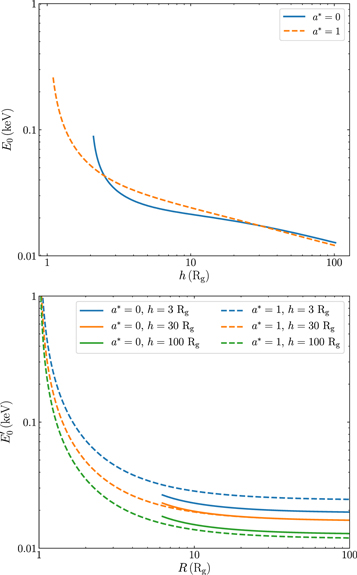
Figure 1. Upper panel: Dependence of the intrinsic rollover energy, E0, on the X-ray corona height. Bottom panel: Plot of the rollover energy,  , as seen by the disk, as a function of radius for several heights. The solid and dashed lines correspond to a* = 0 and 1, respectively. The energies are estimated for a 106 M⊙ BH and an accretion rate of 0.01
  .
.
Download figure:
Standard image High-resolution imageThe rollover energy seen by the disk,  , will be further modified due to the photons' energy shift as they travel from the corona to the disk elements. The bottom panel of Figure 1 shows
  as a function of the disk radius for several corona heights. One can see that its value is below 0.1 keV for the assumed BH mass and accretion rate, except very close to the BH (R ≲ 2 Rg) in the case of a high BH spin, where it can reach ∼0.1 keV (but close to the horizon even up to ∼1 keV).
2.2. The High-energy Cutoff in the X-Ray Spectrum
KPD19 used the xillverD tables (García et al. 2016), which allow the use of different disk densities, but the high-energy cutoff (Ecut) is fixed at 300 keV. In reality, the intrinsic high-energy cutoff can be lower or higher than 300 keV. Even if it is 300 keV,  in the rest frame of a disk ring can be shifted to very high energies for rings close to the event horizon in the case of large heights. It can also be shifted to much lower energies for rings far from the BH in the case of very low heights. Hence, if Ecut is fixed, the incident flux can be over- or underestimated, especially for hard energy spectra (i.e., Γ < 2). Therefore, an alternative possibility is to consider the xillver-a-Ec5 (García et al. 2013, 2014) tables, which are computed for a single disk density of 1015 cm−3 and various Ecut values.
To investigate the significance of  we use the fiducial parameter values listed in Table 1, and we compute the disk response function in the first wave band listed in Table 2 for
  and 0.1. The results are plotted in Figure 2. The solid and dashed lines show the response when we use the xillverD and xillver-a-Ec5 tables, respectively (n = 1015 cm−3 in both cases; the amplitude of the response function is not the same for the two X-ray flash luminosities for reasons we explain in Section 3.6).
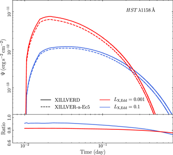
Figure 2. Response functions in the HST λ1158 band, using the xillverD and xillver-a-Ec5 tables with nH = 1015 cm−3 (solid and dashed lines, respectively), in the case of a* = 1. We assume LXobs,Edd = 0.001 and 0.1 (red and blue lines, respectively). The lower panel shows the ratio of the response functions.
Download figure:
Standard image High-resolution imageTable 1. The Parameter Values We Use to Compute the Response Functions
| Parameter | Range | |
|---|---|---|
| BH spin | a* | 0, 1 |
| BH mass | MBH (108 M⊙) | 0.01, 0.05, 0.1, 0.5, 1 |
| Accretion rate |

|
0.005, 0.01, 0.02, 0.05, |
| 0.1, 0.2, 0.5 | ||
| Corona height | h (Rg) | 2.5, 5, 10, 20, 40, 60, |
| 80, 100 | ||
| Photon index | Γ | 1.5, 1.75, 2, 2.25, 2.5 |
| Inclination anglea | θ (deg) | 5, 20, 40, 60, 80 |
| Inner radius | Rin (Rg) | RISCO, 20, 100 |
| Outer radius | Rout (Rg) | 5 × 10², 103, 5 × 10³, 104 |
| X-ray luminosity |

|
0.001, 0.0025, 0.005, 0.01, |
| 0.025, 0.05, 0.1, 0.25, 0.5 |
Note. The numbers in bold font are the fiducial values.
aThe angle between the normal to the disk and the line of sight.Download table as: ASCIITypeset image
Table 2. The Central Wavelengths and Widths for the Different Wave Bands Considered in This Work
| Band | λc (Å) | Δλ (Å) |
|---|---|---|
| HST 1158 | 1158 | 5 |
| HST 1367 | 1367 | 5 |
| HST 1746 | 1746 | 5 |
| UV W2 | 1950 | 600 |
| UV W1 | 2600 | 700 |

|
3580 | 339 |

|
4754 | 1387 |

|
6204 | 1240 |

|
7698 | 1303 |

|
9665 | 2558 |
Download table as: ASCIITypeset image
The amplitude of the response is larger when we use the xillverD tables, at all times, for both the high and the low X-ray illuminating flux. This is because the fiducial (observed) cutoff energy is 150 keV, which implies an intrinsic cutoff of ∼180 keV for a corona located at h = 10 Rg (see Tamborra et al. 2018). This is much lower than the default intrinsic cutoff of 300 keV in the case of the xillverD tables, so we consistently overestimate the incident and the absorbed flux when using these tables.
The difference between the two responses is of the order of 10%–20%, but it will increase for harder spectra (i.e., Γ < 2) or cutoff energies lower than 150 keV. The difference in the amplitude of the response function will reverse when the intrinsic cutoff energy is higher than 300 keV. In this case, using the xillverD tables, we will underestimate the intrinsic and absorbed fluxes, and the response amplitude will be smaller than what it should be. For these reasons, we compute the disk responses with the xillver-a-Ec5 tables (and fix the disk density at 1015 cm−3).
2.3. The Disk Reflection Spectrum
In addition to Finc(R, t), we need to know the disk reflection flux, Fref(R, t), to accurately compute the absorbed X-ray flux. To compute Fref(R, t) we determine the disk ionization (which depends on Finc(R, t) and the disk density, n), and then we use the appropriate xillver tables.
The xillver tables provide the X-ray reflection spectrum at energies above 0.1 keV. If the low-energy cutoff in the rest frame of each disk ring,  , is lower than 0.1 keV, we assume that the incident flux below 0.1 keV is fully absorbed, and we compute Fref(R, t) by integrating the xillver tables above 0.1 keV (as in KPD19). In some rings though,
  is higher than 0.1 keV. This can happen close to the BH (depending on
  , and h; see Equation (5) and Figure 1). We consider two options to address this issue: (1) use the xillver tables with their original cutoff at 0.1 keV or (2) integrate the xillver tables above
  . In the first case we risk overestimating the reflection flux, while in the second approach we could underestimate it. We test several cases with both approaches and we find that the differences in the resulting response functions are negligible. In the rest of the analysis, we estimate the response functions by integrating the xillver tables above
  whenever it is higher than 0.1 keV.
2.4. Comparison with Past Studies
Before presenting our results, we investigate whether our approach in computing Finc(R, t) and Fref(R, t) results in response functions that are significantly different when compared to response functions computed with various approximations that have been commonly assumed in the past.
2.4.1. Constant Albedo versus Self-consistent Reflection from Ionized Disk
In most cases, the disk reflection flux in the past was calculated by assuming a constant disk albedo. To test the importance of computing the disk reflection flux taking into account the disk ionization, as opposed to assuming a constant disk albedo, we consider model parameters in such a way that E0, as seen by the corona and disk, is as high as possible. In this case, we can compute accurately the disk reflection flux and hence the amount of thermalization, as the incident flux below 0.1 keV (the lowest value for the reflection tables) will be minimal.
Thus, we choose a rather extreme case with MBH = 105 M⊙ and  , where the disk temperature and consequently the seed photon energy will be high. To see the effects for different disk ionization states we further set LXobs,Edd = 0.001 and 0.1. For the rest of the parameters we choose Γ = 2 for the primary power-law photon index, h = 10 Rg for the corona position, a* = 1 for the BH spin, and θ = 40° for the system inclination. We consider the case where the reflection flux is computed in a self-consistent way and the case where we fix the thermalized flux to 70% of the X-ray incident flux (equivalent to considering a constant disk albedo of 0.3). All GR effects are taken into consideration in correctly computing the incident X-ray flux in both cases (i.e.,
  ,
,  , and hence Finc(R, t) are computed in the same way in both cases). The results are shown in Figure 3 for four different wave bands.
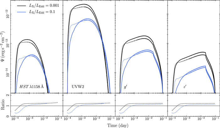
Figure 3. Top panels: Response functions for LXobs,Edd = 0.001 and 0.1 (black and blue, respectively) when the disk reflection spectrum is taken into account including the disk ionization (solid lines) and when assuming an albedo of 0.3 (dotted lines). Bottom panels: The ratio of the response functions for each luminosity (see Section 2.4.1 for details).
Download figure:
Standard image High-resolution imageThis plot shows that computing the reflection spectrum by assuming an albedo of 0.3 overestimates Ψ at early times when Ψ rises, and underestimates it later. This effect is more important when LXobs,Edd is high, as the gradient in the ionization profile of the disk is more important compared to lower X-ray luminosity. It is worth noting that a smaller albedo (i.e., a larger thermalization fraction) will increase the difference seen at early times as it will predict a larger Ψ. The difference in the response function in the two cases will be important in the prediction of the reverberation signal in the various UV/optical wave bands, as the case of a constant albedo will overestimate the predicted flux, especially when the incident X-ray flux is large.
2.4.2. X-Ray Incident Spectrum versus Fixed X-Ray Incident Flux
In most cases in the past, a fixed flux for the X-ray corona was assumed. However, as we mention in Section 2.1, the low- and high-energy cutoffs in the spectrum of the X-ray corona also play a role in determining the X-ray flux that will be absorbed by the disk. In order to highlight the importance of the spectral shape of the primary emission in accurately determining the response functions, we perform the following test.
We consider a BH with a mass of 105 M⊙, LXobs,Edd = 0.001, and the other model parameters set to the fiducial values listed in Table 1. We consider two illuminating X-ray spectra having the same photon index and the same Ecut. In the first case we set E0 (in the intrinsic corona energy spectrum that shines the disk) to the correctly estimated value (as described in Section 2.1). In the second case we fix E0 at 0.5 keV. The normalization of the two energy spectra is set to ensure the total X-ray luminosity (between E0 and 1 MeV) is 0.001 (in Eddington units) in both cases.
The response functions for HST λ1158 Å are shown in Figure 4. The correct E0 for the model parameters we choose is lower than 0.5 keV. As a result, the amplitude of the response function is smaller when E0 is fixed at 0.5 keV, because less soft X-rays are absorbed and thermalized than in reality. This effect is more pronounced in the case of steep photon indices, where the amplitude of the response functions can differ by a factor of 10 or more. Consequently, a fixed X-ray luminosity, without considering all the parameters of the X-ray spectrum, may lead to the calculation of the wrong disk response.
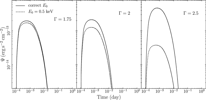
Figure 4. The response functions in the HST λ1158 Å band, estimated by fixing E0 at 0.5 keV (dashed lines) and by estimating E0 correctly. The power-law normalization is set in a way that the total X-ray luminosity is the same in both cases. We show the response functions for different values of Γ (increasing from left to right).
Download figure:
Standard image High-resolution image2.4.3. The Significance of GR Effects
Finally, we investigate the effects of accounting for GR when estimating the photon trajectory from the X-ray source to the disk and also when computing E0 and  . We consider the fiducial model parameters (see Table 1) and two cases for the corona height: h = 2.5 Rg and 100 Rg. We compute the response functions following the same steps, but in the first case we use full GR computations, while in the second case we take a Newtonian approach with photons moving along straight lines and not shifting their energy. In the second case we still assume E0 to be equal to the temperature of the disk spectrum approximation described in Section 2.1 and the intrinsic Ecut to be the same as the observed one. We also take into account the disk ionization effects in both cases.
The response functions are presented in Figure 5. The figure shows that the difference between the two approximations is minimal for the large height. However, for h = 2.5 Rg, the response functions are smaller in amplitude in the Newtonian approximation. This implies that the Newtonian approximation underestimates the reverberating signal in the UV/optical bands. In addition, the Newtonian transfer functions rise (slightly) earlier than those in the case where we consider GR.
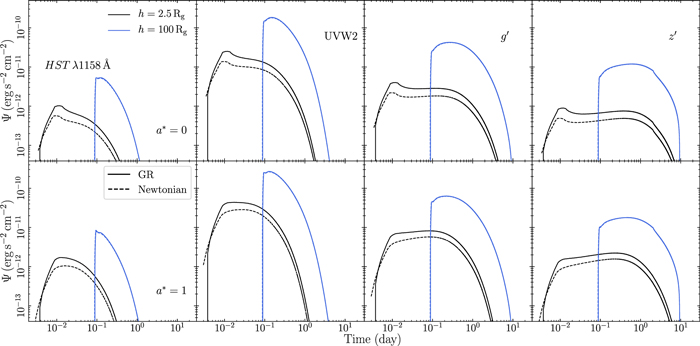
Figure 5. Response functions assuming fiducial parameters and h = 2.5 Rg and 100 Rg (black and blue, respectively) and assuming GR (solid lines) and the Newtonian approximation (dashed lines) for a* = 0 and 1 (top and bottom panels, respectively).
Download figure:
Standard image High-resolution image3. The Disk Response Functions
Table 1 lists all the physical parameters that influence the disk response to an illuminating X-ray source. Our aim is to investigate how these parameters affect the disk response. We use Equation (3) and we compute the disk response for a broad range of values for each parameter, which are listed in the right column of Table 1. The numbers in bold indicate the fiducial parameter values: we keep the parameter values fixed to these numbers when we vary another parameter. For each combination of parameter values, we compute the response for a nonrotating and a maximally spinning BH (a* = 0 and 1, respectively).
We compute the response function in 10 wave bands, as listed in Table 2. The first three are the bands where the far-UV continuum was measured in NGC 5548, using the HST data taken during the Space Telescope and Optical Reverberation Mapping Project (De Rosa et al. 2015; Edelson et al. 2015; Fausnaugh et al. 2016). The next two bands are the Swift/UVOT W1 and W2 bands, and the remaining five bands are representative of the Sloan Digital Sky Survey  filters. The exact central wavelength, λc, and width of the bands are not important at the moment. What is important is that the λc are roughly equidistant from the far-UV to the near-IR. Consequently, the respective responses are representative of the disk response over the full UV/optical spectral band. We plot the response functions for all parameter values in the appendix (Figures 8–15 in Appendix B). For reasons of clarity, we show the response in four bands only (HST λ1158, UVOT/W2,
  , and
, and  ), which are representative of the disk response in the far-UV, UV, optical, and near-IR.
In the following subsections we investigate the dependence of the main properties of the response function, its start time, its width, and its amplitude on the basic parameters of the system.
3.1. The Response Start Time
The response start time, tstart, is the same in all bands because we first detect inner parts of the disk emitting BB radiation with a temperature that corresponds to  Å. This temperature is high enough to contribute even in the shortest wavelengths we consider. The flux in the optical bands is significant even at early times, despite the fact that the disk area we observe at the beginning is small. This is due to the fact that the temperature of the inner disk is quite high (and the flux is proportional to T4).
The disk responds to the X-ray flash at the same time, at all bands, when the geometry is fixed, i.e., for a given BH mass, corona height, and inclination. The response start time, measured in days (and not in Tg = Rg/c), increases linearly with increasing MBH (see also Figure 8 in Appendix B). This is because all the geometries studied and thus all distances and corresponding light travel times are scaled with Rg and Tg, respectively, both of which scale with the BH mass. The response start time also increases with the corona height, h, because the light travel time between the corona and the disk increases accordingly. However, the relation between tstart and h is not exactly linear (Figure 10 in Appendix B). This is due to the fact that photons do not travel along straight lines, especially when h is small, and so the light travel time does not depend linearly on h.
The observer sees the disk responding to the X-ray flash much faster if the inclination is high (Figure 12 in Appendix B). The observed tstart does not change significantly, as long as θ < 40°. But at higher inclinations, tstart decreases fast as θ increases. Although GR contributes to this effect, it arises purely from the same geometrical reasons as in flat spacetime. For higher inclinations, the region that the observer sees responding the earliest moves outward from the center. The difference between the lengths of the light paths for photons coming to the observer directly from the source and for those that are emitted by the disk in this region is much smaller for high inclinations.
It is interesting that the response start time does not depend on the BH spin. For all the parameter values we consider, tstart is identical in the a* = 0 and a* = 1 cases. This implies that we first detect disk elements that are located at distances larger than 6 Rg, even for the lowest corona height we consider (h = 2.5 Rg) for the fiducial inclination of 40°.
3.2. The Width of the Response
The width of the response increases at longer wavelengths. This effect was already noticed by KPD19. The response function in a particular band, λc, starts decreasing when the temperature of the reverberating disk elements is such that the peak wavelength of their BB emission is longer than λc. When this happens, it is the Wien part of the BB spectrum that contributes to the observed flux in this wave band, and it therefore significantly decreases. As time passes, we detect emission from the outer, and thus colder, parts of the disk. They can still contribute significantly in the optical bands, but not in the far-UV bands. Consequently, the width of the response is larger at longer wavelengths. In general, when the overall temperature of the disk is low, the disk response at a given wave band is shifted closer to the BH, and thus the response starts decreasing at earlier times, becoming narrower. Therefore, any change in the system parameters that decreases the disk temperature causes the response width to be shorter.
The discussion above explains the dependence of the response's width on the BH mass and the accretion rate. The width increases with increasing BH mass, but the rate of the increase in response width with BH mass is smaller than the respective linear increase in tstart. This is because as MBH increases, the disk temperature decreases. The same reason also explains the narrowing of the response function as the accretion rate decreases and the overall disk temperature drops (Figure 9 in Appendix B).
As discussed at the beginning of this section, the response at each wave band depends on the disk temperature, and thus it is confined to a disk region up to some radii where the response reaches the Wien part of the spectrum. If we increase the height, the reverberating image of a flash moves through this region faster. Therefore, intuitively one would expect that the width of the response should decrease by increasing the height. However, the opposite is true, and we observe the response width increasing with increasing corona height (see Figure 10 in Appendix B). The wavelengths we consider in this work are long enough that regions with quite large radii still contribute to the response. For example, it is clear from Figure 14 in Appendix B that, for h = 10 Rg, the disk elements just above 1000 Rg still contribute to the responses even at the shortest studied wavelength of 1158 Å. For greater heights even farther regions of the disk contribute to the responses at short wavelengths. Since we explore heights below 100 Rg (i.e., heights smaller than the maximum radius of the reverberating region), the above-described effect of shortening the response is quite weak.
There is, however, another effect in action that enhances the thermalized flux and eventually leads to an increase in the response width with increasing height. The incident flux reaching the disk at large distances R decreases as 1/(h2 + R2) and is proportional to the cosine of the incident angle, which is defined as the angle between the normal to the disk and the photon trajectory. The response width depends on the disk emission at large distances, where R ≫ h. Note that for all the studied wavelengths, it is the contribution from regions of R > 1000 Rg that is crucial for the width of the response, and the maximum height we consider is 100 Rg—thus R > 10 h, at least. At these distances, the incident flux is independent of h (as 1/(h2 + R2) ∼ 1/R2), and the cosine of the incident angle is equal to  . Therefore, as h increases, so does the cosine of the incident angle—and the incident flux as well. Due to the enhancement of the thermalized flux, disk regions further out contribute more, thus effectively prolonging the response time (this effect increases toward longer wavelengths). Disk elements at small radii, where the cosine of the incident angle decreases with increasing height, contribute only at the start time of the response function. Hence they do not affect the width of the response functions.
A change in the photon index, Γ, with the X-ray luminosity in the 2–10 keV band kept the same, changes the shape of the primary power law. When Γ steepens, the flux below 1 keV increases. Since the low-energy cutoff is usually below 0.1 keV, the increase in Γ increases the flux at low energies, which contributes to the disk thermalization. As with the corona height, this effect leads to the response lasting longer (further out regions of the disk start to contribute to the thermal reverberation signal in all bands, even in the shortest ones), as seen in Figure 11 in Appendix B. One can see that the largest change occurs when the power-law index is steepest. The contribution of the primary radiation to thermalization below 0.1 keV changes very slowly for flat Γ.
The width of the response increases with larger inclination angles (see Figure 12 in Appendix B). This is due to the fact that it takes longer to detect emission from the far side of the disk (due to geometrical reasons, as in the case of tstart but with an opposite effect).
3.3. The Amplitude of the Response
We recall that the response function gives the flux of the variable, thermally reverberated disk component (normalized to the illuminating X-ray flux) as a function of time. The integral of Ψ(λc, t) over time is equal to the disk flux due to X-ray heating (in each wave band). The response amplitude increases when the contribution of thermalization to the thermal flux at a given wavelength increases. This can be caused by several effects: (1) an increase of the total incident flux, (2) a decrease of the original NT thermal emission (i.e., by decreasing the disk temperature) while keeping the total incident flux the same, or (3) a low ionization of the disk, which then reflects less. We explore below how the various system parameters may contribute to these effects.
The BH mass can affect the response amplitude in various, and partially opposing, ways: (i) The BH mass scales with the source luminosity, given in units of LEdd, and thus with the normalization of the incident flux (by a factor proportional to MBH). (ii) A larger BH mass decreases the temperature of the disk and so increases the response amplitude. The lower disk temperature also implies lower E0, and the same X-ray luminosity in the 2–10 keV band leads to a larger total incident flux. Since E0 is usually lower than 0.1 keV, this additional flux mainly contributes to the thermalized part, effectively increasing the amplitude of the response. However, (iii) an increase in the total incident flux will further ionize the disk so that it will reflect more efficiently. Therefore, an increased incident flux may also decrease the thermalized part (i.e., it will suppress the magnitude of the effects described above). Figure 8 in Appendix B shows that the response amplitude increases with increasing BH mass, as expected. But it does not increase exactly proportionally to MBH, due to reason (iii) mentioned above.
The response amplitude increases with a decreasing accretion rate (Figure 9 in Appendix B). This is caused by a lower temperature of the accretion disk as we explain in point (ii) above when discussing the effect of BH mass. The response amplitude also increases with greater corona height and steeper Γ. As discussed in the previous section, the thermalized flux increases with increasing corona height and with the steepening of the power-law photon index of the X-ray corona. The inevitable consequence of this effect is an increase in the amplitude of the response function since more flux is emitted at a given wavelength (see Figures 10 and 11 in Appendix B).
Finally, the response amplitude decreases with an increasing inclination angle. This is a projection effect, since we see a smaller overall disk area as the inclination increases. Actually, at inclinations above 40° the response starts to decay at much earlier times. This is due to the fact that the expanding reverberating part of the echo on the near side of the disk (closer to the observer) moves faster outward, outside of the disk region contributing to the given wavelength (see Figure 12 in Appendix B).
3.4. The Effects of BH Spin
For high BH spins, the disk inner edge moves closer to the BH and the disk temperature increases toward the center. However, this has little effect on the response functions. As already discussed, the inner disk region contributes minimally to the response function (in the wave bands we study in this work). The emission from the inner disk affects the response function only at early times, so it does not substantially affect either its width or its amplitude. However, the BH spin affects the disk response in one more way. The spin determines the value of  in physical units (M⊙ yr−1). The accretion rate in these units is higher for low spins (for the same
  ), and the disk is hotter. Hence, for a* = 0, the response functions are broader and have a lower amplitude compared to the response functions when a* = 1.
3.5. The Effects of the Inner and Outer Disk Radii
The effects of changing the inner disk radius (Rin) are shown in Figure 13 in Appendix B. The response functions start at later times as Rin increases because the X-ray photons take more time to reach Rin. At later times, when the outer disk elements contribute to the reverberation signal, the response functions are almost identical to the responses when Rin = RISCO. We note that the response amplitude increases (slightly) with larger Rin because E0 changes with Rin. Therefore, the incident X-ray spectrum and consequently the reverberated flux as well will be slightly different. However, the net effect is an overall decrease of the reprocessed flux as the inner disk radius becomes larger, as we miss an increasing fraction of the X-ray reverberation in the inner disk.
The opposite effect is observed when the outer disk radius (Rout) decreases (Figure 14 in Appendix B). The response functions in this case start at the same time (in all the wave bands). However, Ψ becomes narrower as Rout decreases. This is because the outer disk (which is detected at later times) is missing in this case. This effect is more pronounced at longer wavelengths, due to the fact that the outer disk contributes mainly in the optical/near-IR bands.10 As with Rin, the net effect, mainly at longer wavelengths, is an overall decrease in the variable, reprocessed component.
The change of the response width is more significant when Rout decreases. The start time of the response when Rin increases changes by a few hundredths of a day (Figure 13 in Appendix B; we note that the time axis in all similar figures is logarithmic for reasons of clarity) and is exactly the same in all bands. On the other hand, the changes in the width of the response when the outer disk radius decreases are of the order of many days, even in the UV bands (i.e., in the W2 band, as shown by the second-from-left panels in Figure 14 in Appendix B). This has a significant effect on the expected delays, which are wavelength dependent.
3.6. Dependence on X-Ray Luminosity
X-rays play a major role in thermal reverberation studies. Thus, it is important to understand how the response function depends on the X-ray luminosity. This will help us understand better the relation between X-ray and UV/optical variability in AGN.
Figure 15 in Appendix B shows Ψ for many values of the observed 2–10 keV band luminosity of the X-ray flash,  . We consider 2–10 keV luminosity values, which may be large for AGN,11
but these high values are necessary to reveal clearly the relation between the illuminating X-rays and the disk response. We recall that the disk response is already normalized to
. We consider 2–10 keV luminosity values, which may be large for AGN,11
but these high values are necessary to reveal clearly the relation between the illuminating X-rays and the disk response. We recall that the disk response is already normalized to  (see Equation (3)). So, if the response would simply scale linearly with
  , we would expect the responses in Figure 15 in Appendix B to overlap in all bands. However, this is not the case. This plot shows that the disk response depends on the incident X-ray flux in a nonlinear way.
The response functions (in all bands) decrease in amplitude and broaden in time as  increases. This is mainly caused by the fact that the thermalized flux does not contribute to the response in each wave band in the same way at all times. As
  increases, so does the temperature of the disk elements. At early times, the peak BB emission of the inner disk elements is at wavelengths even shorter than 1158 Å. Therefore, we are in the Rayleigh–Jeans part of the BB spectrum emitted by these elements (at all wave bands). Consequently, the increase in flux (in each wave band) is not proportional to the increase in the incident X-ray flux. Therefore, when we divide the response by the illuminating
  , the ratio decreases. At later times, it is the Wien part that contributes to the flux in each wave band. At the Wien part of the BB emission, the change in flux is larger than the change in the incident X-ray flux. So the increase in the response when the Wien part contributes is stronger than the increase in
  . Hence, when we normalize the response with
  , the response is larger with increasing
  at later times. This effect explains the larger width of the responses with increasing
  . For example, in the top rightmost panel of Figure 15 in Appendix B, for the longest wavelength, the
  band, the response does not reach the Wien part at the disk outer radius, Rout, and thus the response does not increase with the X-ray luminosity even when it starts fading (the effect is visible but tiny in the case of a* = 1, where the disk is colder).
There is yet another effect contributing to the response amplitude change with X-ray luminosity. This effect exhibits itself mainly at the beginning of the response when the inner parts of the disk reverberate. Increasing the X-ray luminosity increases Finc(R, t). This leads to an increase in the ionization of the innermost parts of the disk and the fraction of the disk's reflection flux (i.e., Fref(R, t)). The reflection flux increases faster with the disk ionization than the incident flux, due to higher disk reflectivity. Therefore, overall, the absorbed X-ray flux increases slower than  , and when we plot the disk responses normalized to
  , their amplitude will decrease as we increase the incident X-ray luminosity, at early times. At later times, we detect emission from the outer disk. At far enough distances from the center, the illuminating X-ray flux, which generally decreases as ∼1/R2, is always small enough that the disk is neutral, and thus this effect dies out at longer response times.
3.6.1. Implications of the Nonlinear Disk Response
The nonlinear disk response to the illuminating X-rays complicates the modeling of thermal reverberation in AGN. Equation (4) is valid, but if the disk response function depends on the incident X-rays, the convolution integral will be difficult to solve as Ψ must change continuously, according to the variable input LX. This may be important when using Equation (4) and the observed X-rays to predict model UV/optical light curves (in all wave bands). In order to explore this issue, we use the response functions plotted in Figure 15 in Appendix B, and we compute their ratio when the ratio of the incident X-ray luminosity is equal to 2. The results are plotted in Figure 6.
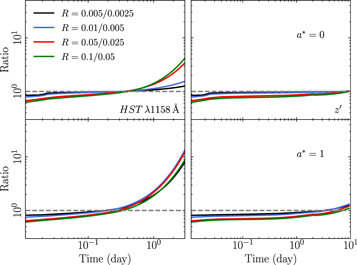
Figure 6. Ratio of response functions in the HST λ1158 and  bands (left and right columns) with spins of 0 and 1 (upper and lower rows, respectively). See Section 3.6.1 for details.
Download figure:
Standard image High-resolution imageThe ratio of the responses is relatively flat in the optical band, for both spin 0 and spin 1 (right plots in Figure 6). The ratio is between 0.6 and 0.8 at early times, because the response amplitude decreases when the X-ray luminosity increases (as discussed above). There is a trend of the ratio increasing at later times (because the width of the response increases), but it is not very strong.
The plots indicate that it may be possible to use Equation (4) with Ψ equal to the disk response to the mean X-ray luminosity. For example, let us suppose that a source varies by a factor of 4 in the 2–10 keV band, say, from 0.0025 to 0.01 (in Eddington units; black and blue curves in Figure 6) or from 0.025 to 0.1 (red and green curves in the same figure). Let us now assume that we use the response function for  and 0.05 in Equation (4). This X-ray luminosity is almost equal to the mean of the minimum and maximum values (in both cases). The use of a fixed response in Equation (4) means that we will be overestimating/underestimating the reverberating flux when the X-ray luminosity is higher/lower than the mean. But according to the black/blue and red/green lines in the right plots of Figure 6, we will over/underestimate the flux by almost the same factor each time. Therefore, the resulting reverberating flux should be approximately correct, on average. The left panels of Figure 6 show the disk response functions in the far-UV band. Here, the changes in the response width with incident X-ray flux are more pronounced at timescales longer than about 1 day. However, the black/blue and red/green lines are still (almost) identical. We therefore believe that the arguments above can still apply in this case.
We investigate in Appendix A the nonlinear disk response to X-rays in more detail. Our results show that, even if X-rays vary by a factor up to 10, we can use the disk response that corresponds to the mean X-ray luminosity in Equation (4) to estimate model UV/optical light curves and to model time lags and reverberation fractions (see the following sections for the definition and modeling of these quantities).
4. Application to Observations
The model disk responses can be used to study the X-ray–UV/optical correlation. One possibility is to use Equation (4) and the observed X-rays in order to produce model UV/optical light curves and compare them with the observed ones. This would be the best way to test the validity of the model assumptions and to constrain the disk/corona geometry. However, this is a formidable task.
The sampling rate of the X-ray light curves is crucial for the proper estimation of the X-ray-reprocessed UV/optical flux. If the average cadence of the X-ray light curve is larger than the timescale when the bulk of the UV/optical flux is emitted, interpolation of the X-ray light curve will be necessary. For example, Figure 8 in Appendix B shows that the UV W2 response decreased to 10% of its maximum amplitude after ∼0.6, 1.5, and 3 days in the case of 107, 5 × 10⁷, and 108 M⊙. Therefore, we need an X-ray sampling rate at least 10 times smaller, roughly speaking, in order to be able to compute the integral in Equation (4) correctly for this band. We would need an even denser sampling if we wish to compute the model flux at shorter wavelengths (the constraint is more relaxed of course at longer wavelengths). This would of course also depend on the X-ray variability amplitude, but it is possible that the resulting UV/optical light curves may tell us more about the way the interpolation was done than about the physical properties of the source.
Another way to compare the model predictions with data is through power spectral density (PSD) analysis. Equation (4) predicts a unique relation between the X-ray and the UV/optical PSDs (see, e.g., Panagiotou et al. 2020). The most common method for studying the X-ray and UV/optical correlation is cross-correlation analysis of multiwavelength monitoring observations. Cross-correlation techniques are used to estimate time lags between the observed X-ray, UV, and optical light curves as a function of the wavelength. We use the model disk transfer functions presented in the previous section, and we compute the model time-lag spectra for all the model parameters we consider in this work. We present our results below.
4.1. Cross-correlation and Time Lags
The response function determines, to a large extent, the cross-correlation between the X-ray and the UV/optical light curves. It is commonly accepted that the centroid of the response function, τcen, is representative of the maximum peak in the cross-correlation function (CCF) that is measured between the X-ray and the UV/optical light curves. The centroid is defined as follows:

We note that this is an approximate measure of the CCF peak, because the CCF is the convolution of the transfer function and the continuum autocorrelation function (e.g., Equation (12) in Peterson 1993),

where ACFX is the autocorrelation function of the X-ray light curve. The X-ray PSDs have a power law–like shape that extends to very low frequencies with a slope of ∼−1 (e.g., McHardy et al. 2004, for NGC 4051). This implies a long memory and hence a broad X-ray ACF. Consequently, the X-ray ACF should affect the value of the time lag between the X-ray and the UV/optical light curves. However, the X-ray ACF is common to the CCF between X-rays and any UV/optical band, and it should affect all CCFs in the same way, i.e., we would expect the X-ray ACF to produce the same systematic effect on all CCFs. Therefore, we believe that the X-ray ACF may less significantly affect the time lags between a reference band in the UV and any other UV/optical light curve. We would expect time lags within the UV/optical light curves to depend mainly on the disk response function and not on the X-ray ACF.
We use Equation (6) and the model disk responses to compute the model time-lag spectra for all the model parameters. The respective plots are shown in the appendix (Figures 17–23 in Appendix B). In general, τcen increases with increasing wavelength, because the width of the disk response increases with the wavelength (for all parameters).
The slope of the τcent versus λ relation depends on the corona height (see Figure 18 in Appendix B). When the corona is located close to the BH, the slope of the time-lag spectrum is ∼1.34, i.e., equal to the "canonical" slope of 4/3 that is expected in the case of a pointlike corona located close to the BH, illuminating an NT disk. As the corona height increases, the time lags increase at all wavelengths. But they increase more at shorter wavelengths, because the width of the response increases more at shorter wavelengths. As a result, the slope of the time-lag spectra flattens. For example, when h = 100 Rg, the slope is ∼1.1.
The time lags increase with increasing BH mass, accretion rate, and X-ray luminosity. These three parameters affect the normalization of the τ versus λ relations, but not the slope, because they affect the width of the transfer functions by the same factor at all wavelengths. The time-lag spectra increase as the spectral slope Γ steepens, because the width of the response function increases accordingly (Section 3.2). Interestingly, the time-lag spectra do not depend on the inclination. As the inclination increases, the response start time decreases, the width increases, and the response amplitude decreases (see Figure 12 in Appendix B). But apparently, all these changes happen in such a way that the centroid of the response is not affected. It is as if the time lags are set by the physical properties of the system and do not depend on the viewing angle.
The time-lag spectra do not depend significantly on Rin. As discussed in Section 3.5, as Rin increases, so does the rise time of the disk response. The effect is more pronounced in the UV bands. This shift in the rise time leads to an increase in the centroid of the response function (and hence of τ), as seen in Figure 21 in Appendix B. But the effect is subtle and can be seen only when the inner radius is at least 100 Rg. On the other hand, Rout has a profound effect on the time lags (see Figure 22 in Appendix B). The time-lag spectra flatten significantly as the outer radius decreases. In fact, Rout is the only parameter that can cause a flattening of the time-lag spectra even at wavelengths shorter than 5000 Å. This is due to the fact that the width of the disk response is significantly shortened, even at short wavelengths, as Rout decreases. Figure 22 in Appendix B shows that time-lag spectra can be very flat if the outer disk radius is smaller than 5000 Rg. Observed time-lag spectral slopes of the order of ∼0.5 (like those of NGC 4593; see McHardy et al. 2018; Edelson et al. 2019) can be explained by the model, but only if Rout is smaller than ∼5000 Rg.
4.2. An Analytic Prescription for the Time-lag Spectra
We fit all the model time-lag spectra and find that the following equation describes our results well:

where λ1950 is the wavelength normalized to 1950 Å, h10 is the height of the lamp post in units of 10 Rg, M7 is the BH mass in units of 107 M⊙,  is the accretion rate in units of 5% of the Eddington limit, LX,0.01 is the observed 2–10 keV luminosity in units of 0.01 of the Eddington luminosity, and


in the case where a* = 1 and


in the case where a* = 0.
These equations are valid for the time-lag spectra when λ ≤ 5000 Å because the time-lag spectra flatten at longer wavelengths for certain combinations of the model parameters. In all these cases, the disk is hot enough to contribute to the disk response at long wavelengths, even at radii larger than 104 Rg. Since this is the largest Rout we consider, the responses at these wavelengths show an abrupt cutoff at long timescales, and the respective time lags would be smaller than the values if we considered a larger outer disk radius.
Equation (8) shows that the time lags depend on many parameters in a nonlinear way. Of course one can always fit a simple power-law function to the observed data, but the use of Equation (8) to fit the observed time-lag spectra could be more beneficial. In fact, as long as a BH mass estimate is available and an average observed 2–10 keV X-ray luminosity can be determined by X-ray observations of a source, it is straightforward to use Equation (8) to fit the observed time lags and determine the  values that could fit the data best.
4.3. Reverberation Fraction
Although the reverberation signal has been seen in a few sources so far, some AGN, which are very variable in X-rays, do not show any correlation between X-rays and the UV/optical band (see, e.g., Pawar et al. 2017; Buisson et al. 2018; Morales et al. 2019). This could be due to the fact that thermal reverberation does not take place in these sources or is too weak to be detected.
To investigate this issue, we define the reverberation fraction,  , as the ratio between the average reverberated flux and the total (reverberated plus NT) disk flux in a given wave band:
We compute  for all the model parameters, and we present the results in Figures 24–31 in Appendix B.
The reverberation fraction depends on the incident X-ray flux, the amplitude of the response function, and the temperature of the accretion disk. In some cases, this ratio is close to one, which means that the flux in these wave bands is dominated by the flux generated by X-ray absorption. Objects with physical parameters that predict large  will be ideal targets for the study of the X-ray and UV/optical correlation.
A small decrease in  can be seen with increasing λ in almost all cases. In addition,
  is larger for a rotating BH compared to the Schwarzschild case. This is due to the fact that for the same
  in Eddington units, the accretion disk is hotter for lower spins, and hence FNT(λc) is larger and the reverberation signal is smaller. It appears then that it is better to search for the reverberation signal at shorter wavelengths in maximally rotating BHs.
For a fixed BH mass, the UV/optical flux due to X-ray heating (thus  as well) increases with increasing X-ray flux, increasing corona height (because the response amplitude increases with height, as explained in Section 3.3), and decreasing accretion rates (because the disk becomes colder). The reverberation fraction also increases as the spectrum steepens, because the X-ray flux absorbed by the disk also increases in this case. For fixed LX,Edd and
  (in Eddington units), the amplitude of the response functions increases with increasing BH mass (Figure 8 in Appendix B). The flux of the NT disk increases as well. As a result,
  increases with mass, albeit with a moderate rate (Figure 24 in Appendix B).
The inner and outer disk radii also affect the reverberation fraction, although not significantly. The strength of the reverberation component at optical wave bands decreases as Rout becomes smaller (Figure 30 in Appendix B). This is because the response function becomes narrower with decreasing Rout, so its integral over time decreases accordingly. The reverberation fraction increases when Rin gets larger (Figure 29 in Appendix B). This is because the disk flux decreases when considering larger values of Rin. However, the effect is not very strong.
The model-predicted reverberation fraction can be used to explain the results from monitoring campaigns of some X-ray-bright, highly variable NLS1s, such as IRAS 13224–3809 (Buisson et al. 2018), Mrk 817 (Morales et al. 2019), and 1H 0707–495 (Robertson et al. 2015; Pawar et al. 2017). The data show very weak, or even absent, UV/optical variability, while the X-rays are highly variable.
According to our model, the absence of a significant correlation between X-ray and UV/optical bands could be explained when the reverberation fraction is small. This is to be expected in the case of a low corona height and high accretion rate. For example, according to Figure 26 in Appendix B,  ≲ 0.55 and ≲0.2 in the case of spin 1 and 0, respectively, when h ≤ 5 Rg and the accretion rate is 5% of the Eddington limit (the fiducial value). However, if the accretion rate increases to 50% of
  , the reverberation fraction will decrease to ∼0.15 and 0.02 of the total flux (slightly less significantly in the far-UV than in the other wave bands) in the case of spin 1 and 0, respectively. In this case, it will be difficult to detect significant variations in the total observed flux.
5. Summary and Discussion
We have presented the results from a detailed analysis of thermal reverberation in the UV/optical bands caused by the X-ray illumination of the disk by a pointlike X-ray source in AGN. We have considered a number of possible physical parameters that can affect the disk response to X-ray illumination. The main inputs to our code are the observed 2–10 keV X-ray luminosity (in Eddington units), the spectral slope (Γ), and the observed high-energy cutoff (Ecut,obs). We have considered all the appropriate GR effects and determined (1) the intrinsic X-ray luminosity and high-energy cutoff,  , as well as the low-energy cutoff, E0, of the corona (using the respective observed values, MBH,
  , and the height h) and (2) the incident X-ray spectrum at each disk element (in its rest frame). The model then computes the appropriate reflection spectrum, taking into consideration the ionization state of each disk element. In this way, the model accurately computes the incident and the reflected flux—hence the flux that the disk absorbs. We have compared our model disk responses with responses that we computed ignoring GR and/or disk ionization effects (as is frequently the case in past studies). We have found that ignoring those effects can significantly alter the disk response.
We have computed disk response functions in various wave bands. Table 3 lists all the model parameters and how they affect the main characteristics of the disk response functions (i.e., amplitude, start time, and width). Our results show that the disk response to the corona luminosity is nonlinear, due to the nonlinear response of the disk thermalization to the variable X-ray illumination. We have also investigated the effect of the inner and outer disk radii on the response functions. An inner disk radius that is larger than the ISCO radius may be relevant in cases where an extended warm corona with a large optical depth may be present on top of the inner disk (see, e.g., Mehdipour et al. 2011, 2015; Petrucci et al. 2013; Mehdipour & Costantini 2018; Porquet et al. 2018; Petrucci et al. 2020; Matzeu et al. 2020, and references therein). In that case, due to the high optical depth, all the UV/optical photons from the innermost regions of the accretion disk will be shifted to soft X-rays, and the reverberation signal will be observed from disk radii that are larger than the radius of the warm corona. The main effect of increasing Rin is an increase in the rise time of the response, which implies that the amplitude of the reverberating component will decrease (this may be important when predicting the reverberating signal, especially in the UV bands).
Table 3. A Qualitative Summary of the Effects of Each of the Parameters Studied in This Work on the Response Function Amplitude, Start Time, and Width and on the Time Lag and Reverberation Fraction
| Parameter | Ψ | τcen |

|
||
|---|---|---|---|---|---|
| Amplitude | Start Time | Width | |||
| a* ↗ | ↗ | ⋯ | ↘ | ↘ | ↗ |
| MBH ↗ | ↗ | ↗ | ↗ | ↗ | ↗ |

|
↘ | ⋯ | ↗ | ↗ | ↘ |
| h ↗ | ↗ | ↗ | ↗ | ↗ | ↗ |
| Γ ↗ | ↗ | ⋯ | ↗ | ↗ | ↗ |
| θ ↗ | ↘ | ↘ | ↗ | ⋯ | ⋯ |
| Rin ↗ | ↘ | ↗ | ↘ | ↗ | ↗ |
| Rout ↗ | ⋯ | ⋯ | ↗ | ↗ | ↗ |
| LXobs,Edd ↗ | ↘ | ⋯ | ↗ | ↗ | ↗ |
Download table as: ASCIITypeset image
We have used the response functions and computed model time lags and the reverberation fraction  (i.e., the reverberated flux over the total flux). This ratio can be used to explain the lack of UV/optical variability in the case of a few AGN that are highly variable in X-rays. Our results indicate that in the case of low heights and high accretion rates, the reverberating signal can have a very small amplitude that will make it difficult to detect and to study its variability.
The time lags are affected by all the physical parameters that influence the disk response as well. Table 3 summarizes the effects of the model parameters on the time lags and  . In some cases, the model time-lag spectra flatten at longer wavelengths, but this is due to the fact that we have considered an outer disk radius of 104 Rg. A larger Rout will eliminate this effect. However we note that very flat time-lag spectra can be explained within the context of X-ray irradiation of accretion disks, but only if Rout is ∼1000 Rg (or smaller). This possibility implies that time-lag spectra can impose constraints, and in fact, in some cases, they may be used to measure the size of the accretion disk.
The model time-lag spectra we have computed can be used to fit observed time-lag spectra; however, there is a simpler way for this. We have derived an analytic expression for the time lags as a function of wavelength. Equation (8) can be used to fit the observed time-lag spectra at wavelengths shorter than ∼5000 Å. This will provide best-fit values for important physical parameters of the system, like the accretion rate and the corona height, as long as an accurate BH mass estimate is available. The luminosity term in this equation refers to the average observed 2–10 keV luminosity, so it should be easily determined by the observations.
Finally, our results indicate that any variability in the system will be imprinted in the time-lag spectra. In particular, long-timescale changes of the height of the corona, the observed X-ray luminosity, or the disk accretion rate for a given source will change the amplitude of the time-lag spectrum (and its slope, in the case of a variable height). These changes can be revealed through multi-epoch monitoring of bright sources.
Data Availability
The KYNXILREV code used to compute the response functions is publicly available at https://projects.asu.cas.cz/stronggravity/kynreverb/. All the response functions and data presented in this paper are available upon request.
M.C.G. and M.D. acknowledge support from MEYS of the Czech Republic through the 18-00533S research project. M.C.G. acknowledges funding from the European Space Agency through a partnership with IAA-CSIC (Spain). M.D. thanks his home institution, ASU, for their support through the project RVO:67985815. E.S.K. and I.E.P. would like to thank ASU for their hospitality. I.E.P. acknowledges the support of the International Space Science Institute, Bern. The figures were generated using Matplotlib (Hunter 2007), a PYTHON library for publication of quality graphics.
Software: Matplotlib (Hunter 2007), SciPy (Virtanen et al. 2020).
Appendix A: The Nonlinear Disk Response to X-Rays
To study the effects of the nonlinear disk response to the incident X-rays, we perform the following experiment. We consider an X-ray light curve with a maximum-to-minimum ratio of 5 (the "low-var" case) and a light curve with a maximum variability amplitude of 10 (the "high-var" case). We use the fiducial parameters listed in Table 1, and we assume a maximally spinning BH. The light curves are 8.5 days long, with Δt = Tg.
We construct 1000 light curves in each case. The low-var and high-var light curves are a random series of  values of 0.001, 0.0025, or 0.005 and of 0.001, 0.005, or 0.1, respectively. Each value is chosen randomly, with equal probability. For each light curve, we use Equation (4), and we estimate the HST λ1158 and g'-band model reverberation light curves twice: in the first case we consider the exact response function for each
  , while the second time we assume the response of the "intermediate" X-ray luminosity, being 0.0025 and 0.005, respectively.
The solid and dotted red lines in Figure 7 show the mean ratio of the light curves obtained by assuming the response function of the intermediate X-ray luminosity to the light curves computed by using the exact response functions in the low-var and high-var case, respectively. We show the ratio 3 days after the first X-ray flash, when the UV/optical flux has reached an equilibrium state. The results show that the model predictions when we use the exact responses and when we use the response for the intermediate X-ray flux differ by ∼5%–6%, even if the X-rays vary by a factor of 10.
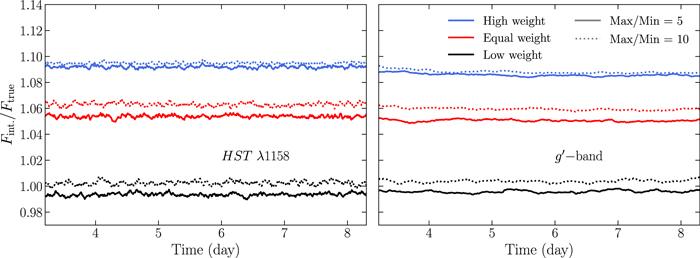
Figure 7. The ratio of the reverberation light curves obtained by assuming the disk response corresponding to the intermediate X-ray luminosity to the correct response function for a maximum-to-minimum X-ray variability of 5 and 10 (solid and dotted lines, respectively). We assume that the source is most of the time in its lowest flux state, in its highest flux state, or with an equal probability in all flux states (black, blue, or red lines, respectively). The ratios are shown in the HST λ1158 and  bands (left and right, respectively). See Appendix A for more details.
Download figure:
Standard image High-resolution imageWe repeat the same test by assigning different weights on  . We consider two scenarios where the X-ray source is in a "faint" or "bright" state for most of the time. To do so, the three
  values mentioned above are not chosen randomly anymore, but with a probability of [60%, 30%, 10%] and [10%, 30%, 60%], respectively. We again construct 1000 light curves, and we compute the mean ratio between the model-predicted reverberation fluxes when we consider the exact responses and the response of the mean X-ray flux. The results are shown in the same figure (black and blue lines for the bright and faint states, respectively; solid and dotted lines for the low-var and high-var light curves, respectively). We note that the scatter of the 1000 simulated ratios around the plotted (average) ones is in the order of 0.6%–1% and 0.2%–0.4% only for the HST λ1158 and g' bands, respectively.
Our results show that, regardless of the X-ray variability amplitude, by assuming the response for the intermediate X-ray luminosity, we overpredict the reverberation signal in the far-UV and optical bands by no more than ∼9% if the source is in a bright state most of the time. If the source is in a faint state for most of the time, the model reverberation flux will differ by less than ∼1% of the exact model value when we assume the disk response to the intermediate X-ray flux.
Appendix B: Plots
In this section we present the plots of the response functions (Figures 8–15), the time-lag spectra (Figures 16–23), and the reverberation fraction (Figures 24–31) for different parameters.
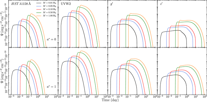
Figure 8. Response functions for all BH masses we consider in this work (see Table 1) in four different wave bands considering spins of 0 and 1 (top and bottom panels, respectively).
Download figure:
Standard image High-resolution image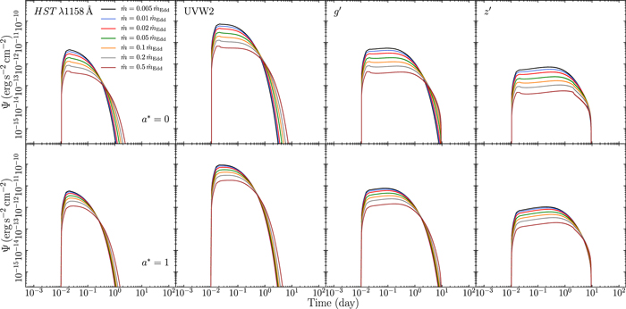
Figure 9. Same as Figure 8, but for the accretion rate.
Download figure:
Standard image High-resolution image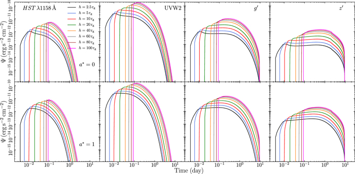
Figure 10. Same as Figure 8, but for the lamp-post height.
Download figure:
Standard image High-resolution image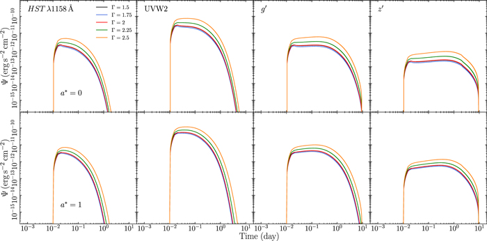
Figure 11. Same as Figure 8, but for the photon index.
Download figure:
Standard image High-resolution image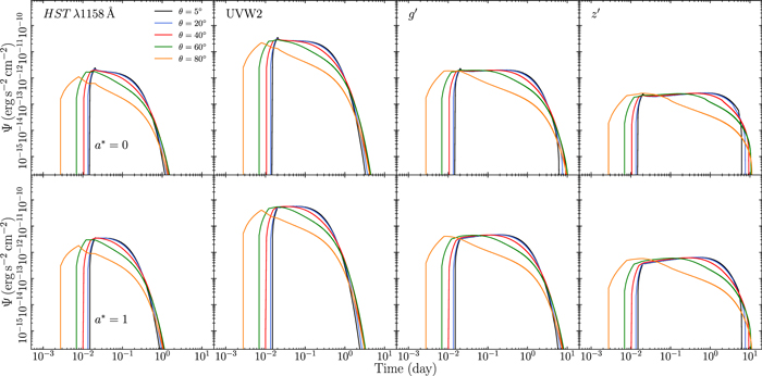
Figure 12. Same as Figure 8, but for the inclination angle.
Download figure:
Standard image High-resolution image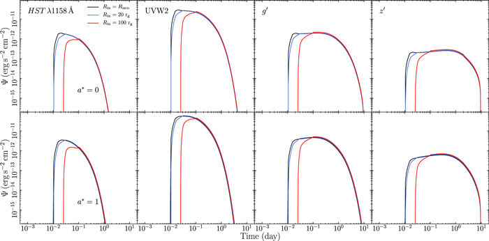
Figure 13. Same as Figure 8, but for the inner radius of the disk.
Download figure:
Standard image High-resolution image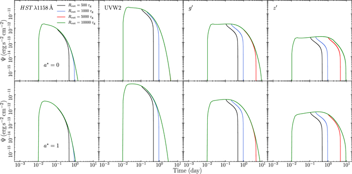
Figure 14. Same as Figure 8, but for the outer radius of the disk.
Download figure:
Standard image High-resolution image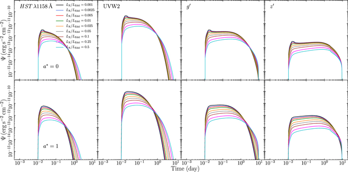
Figure 15. Same as Figure 8, but for the X-ray luminosity.
Download figure:
Standard image High-resolution image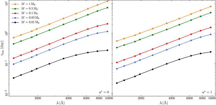
Figure 16. The centroid of the CCF (τcen) as a function of wavelength for different values of the BH mass, considering spins of 0 and 1 (left and right panels, respectively).
Download figure:
Standard image High-resolution image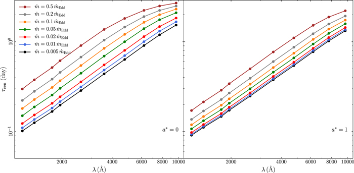
Figure 17. Same as Figure 16 but for the accretion rate.
Download figure:
Standard image High-resolution image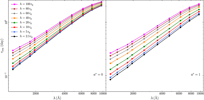
Figure 18. Same as Figure 16 but for the lamp-post height.
Download figure:
Standard image High-resolution image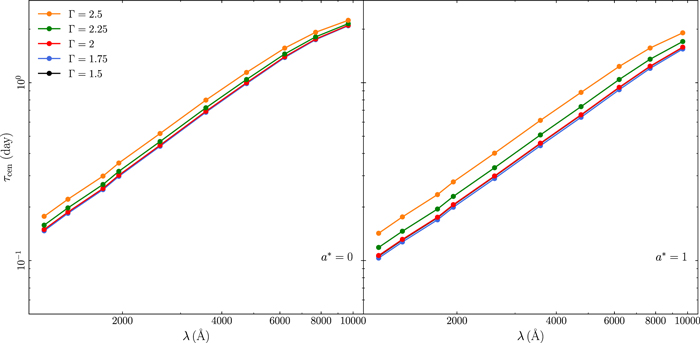
Figure 19. Same as Figure 16 but for the photon index.
Download figure:
Standard image High-resolution image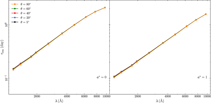
Figure 20. Same as Figure 16 but for the inclination angle.
Download figure:
Standard image High-resolution image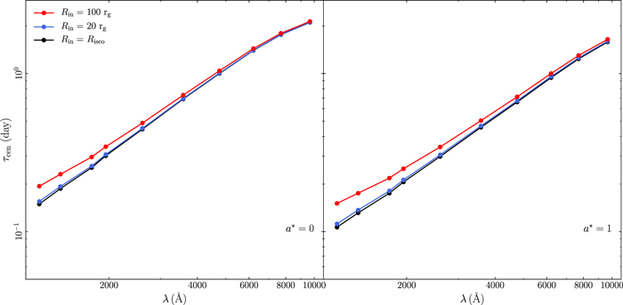
Figure 21. Same as Figure 16 but for the inner radius of the disk.
Download figure:
Standard image High-resolution image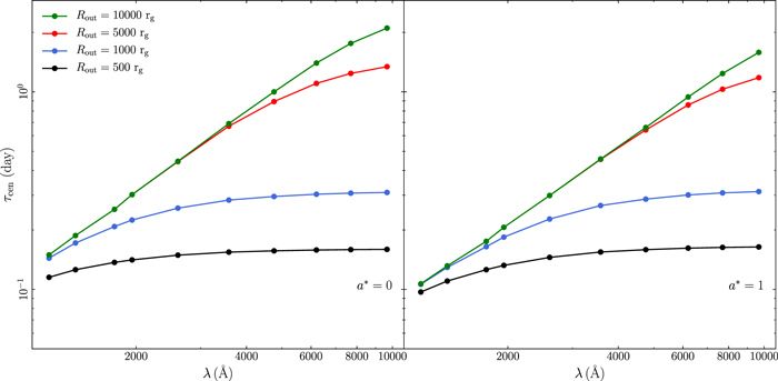
Figure 22. Same as Figure 16 but for the outer radius of the disk.
Download figure:
Standard image High-resolution image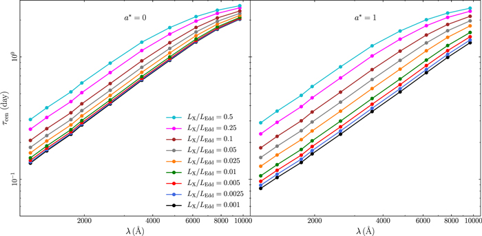
Figure 23. Same as Figure 16 but for the X-ray luminosity.
Download figure:
Standard image High-resolution image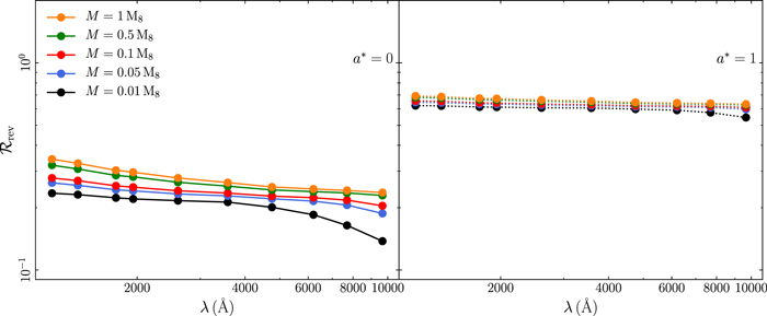
Figure 24. The reverberation fraction plotted as a function of the wavelength for different values of BH mass, considering spins of 0 and 1 (left and right panels, respectively).
Download figure:
Standard image High-resolution image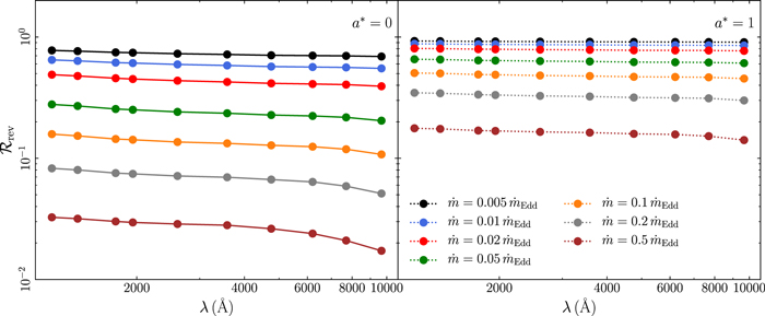
Figure 25. Same as Figure 24 but for the accretion rate.
Download figure:
Standard image High-resolution image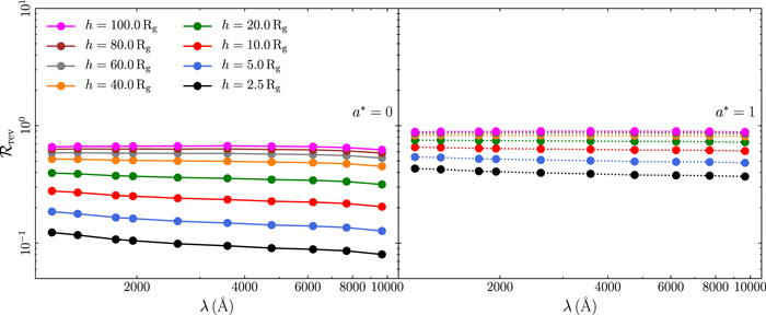
Figure 26. Same as Figure 24 but for the lamp-post height.
Download figure:
Standard image High-resolution image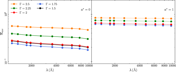
Figure 27. Same as Figure 24 but for the photon index.
Download figure:
Standard image High-resolution image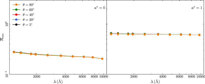
Figure 28. Same as Figure 24 but for the inclination angle.
Download figure:
Standard image High-resolution image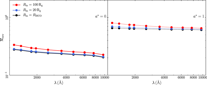
Figure 29. Same as Figure 24 but for the inner radius of the disk.
Download figure:
Standard image High-resolution image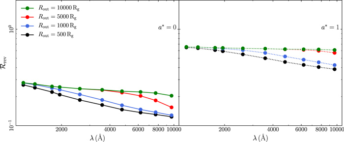
Figure 30. Same as Figure 24 but for the outer radius of the disk.
Download figure:
Standard image High-resolution image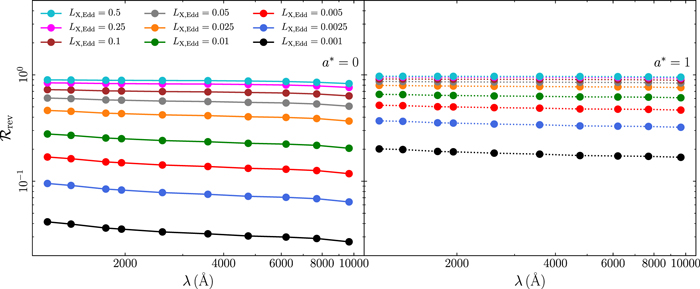
Figure 31. Same as Figure 24 but for the X-ray luminosity.
Download figure:
Standard image High-resolution imageFootnotes
- 5
The dimensionless spin parameter, defined as a* = Jc/GM2, where J is the angular momentum of the BH, is smaller than or equal to 1 (see, e.g., Misner et al. 1973).
- 6
A wave band is determined by its centroid wavelength, λc, and its width
 .
. - 7 is the sum of the blackbody fluxes of the disk elements, each with its own temperature Tnew.
- 8
The NT disk flux is constant with time, but
changes with time since it corresponds to the NT thermal flux produced by the evolving reflection image on the disk . - 9
We remind the reader that the radiative efficiency η is lower for low spins; hence
in physical units is higher for low spins. - 10
In fact, the response functions in the z' band appear to stop "abruptly" in all the cases we consider, mainly because the outer parts of the Rout = 104 Rg disk, for the parameters values we consider, are still quite "warm" and they contribute a noticeable flux in the near-IR bands.
- 11
According to Figure 10 in Lusso et al. (2012), the (observed) 2–10 keV luminosity in AGN can be up to 0.1 of the Eddington luminosity.


![${[R,\phi ]}_{{t}_{\mathrm{obs}}}$](https://content.cld.iop.org/journals/0004-637X/907/1/20/revision1/apjabcb93ieqn9.gif)
