


Abstract
We report 6 yr monitoring of distant bright quasar CTS C30.10 (z = 0.90052) with the Southern African Large Telescope. We measured the rest-frame time lag of  days between the continuum variations and the response of the Mg ii emission line, using six different methods. This time delay, combined with other available measurements of Mg ii line delay, mostly for lower-redshift sources, shows that the Mg ii line reverberation implies a radius–luminosity relation very similar to the one based on a more frequently studied Hβ line.
Export citation and abstract BibTeX RIS
1. Introduction
Broad emission lines coming from the broad-line region (BLR) are the most characteristic properties of most active galactic nuclei (AGNs). The innermost region of the accretion flow in bright AGNs, including the BLR, is spatially unresolved, with the exception of the first image of the BLR in 3C 273 achieved with GRAVITY (GRAVITY Collaboration et al. 2018). Nevertheless, observations of BLR, in particular time variability, allow us to gain an insight into the structure of the nuclear region, provide a tool to measure the black hole mass, and contain a promise of possible cosmological applications.
The first image of the BLR seen with GRAVITY in general supports the view that was formulated before: the BLR forms a flattened structure with the symmetry axis aligned with the jet axis, and the velocities of the clouds are predominantly Keplerian, roughly consistent (within a factor 2) with the result obtained from traditional reverberation mapping by Zhang et al. (2019).
Thus, reverberation mapping is a reliable method of measuring the size of the BLR and the black hole mass (Kaspi et al. 2000; Peterson et al. 2004; Mejía-Restrepo et al. 2018). The mass determination requires the measurement of the time delay between a given line and a continuum, the measurement of the line width (either FWHM or σ), and the knowledge of the virial factor. Observations suggested a strong coupling between the BLR size obtained from such delay measurements and the monochromatic luminosity (Kaspi et al. 2000; Bentz et al. 2013), and such a generalized law leads to single-spectrum methods of black hole mass calculations in large quasar catalogs (e.g., Shen et al. 2011).
However, most of the measurements were done only for relatively nearby AGNs, in the Hβ line. In the case of more distant quasars, their Hβ line moves to the IR domain, and optical observations provide only the UV part of the spectrum with Mg ii and C iv lines. There were attempts to bridge the use of Hβ and other lines by taking into account the systematic differences in the line widths, as well as due to the fact of using also a different part of the continuum as a reference (see, e.g., Woo et al. 2018). Statistical scaling, however, has some limitations, particularly that higher-redshift sources have frequently higher masses and/or Eddington ratios, so the direct confirmation of the scaling laws from reverberation mapping in lines other than Hβ is important.
In this paper we present our reverberation campaign in the Mg ii line of quasar CTS C30.10 (z = 0.90052). Mapping in Mg ii is more difficult since the variability of the Mg ii line is in general lower than in Hβ (Goad et al. 1999; Zhu et al. 2017). There are only a few successful measurements in this line so far. Clavel et al. (1991) pioneered the reverberation mapping in the UV lines, but the constraints they received for NGC 5548 were very approximate, ∼34–72 days for the Mg ii line. The first firm delays, in two epochs, were measured for NGC 4151 by Metzroth et al. (2006). Shen et al. (2016) reported the time delay measurement in Mg ii for six objects at moderate redshift (between 0.4253 and 0.7510), and all their sources were of relatively low luminosity  below 44.416). Lira et al. (2018) report the delay for the quasar CTS 252 (z = 1.818,
  ). Cackett et al. (2015) performed monitoring of NGC 5548 in UV, but they were not able to determine the Mg ii time delay from their data. Our campaign lasted 6 yr, and we are able to report the definite delay measurement for a more distant and very bright quasar (
 ). Very preliminary results of this effort were published in a short conference report (Czerny et al. 2018).
2. Observations and Data Reduction
Quasar CTS C30.10 has been found in the Calan-Tololo Survey, as part of a survey aimed at finding new bright quasars in the southern part of the sky (Maza et al. 1988, 1993). The source is located at R.A. = 04h47m19 9, decl. = −45d37m38s (J2000.0). Quasar identification has been confirmed by Maza et al. (1993). The source is bright (V = 17.2, as given by NED), and the redshift (z = 0.910 in NED) has been revised to z = 0.9000 by Modzelewska et al. (2014). The source has been observed with the Southern African Large Telescope (SALT) from 2012 December 6 until 2018 December 10.
2.1. Spectroscopy
The source was observed in a slit spectroscopy mode, using the Robert Stobie Spectrograph (RSS; Burgh et al. 2003; Kobulnicky et al. 2003; Smith et al. 2006) in the service mode. We collected 26 observations, each consisting of two observing blocks, with exposures lasting ∼800 s. A slit width of 2'' was used, as well as RSS PG1300 grating, which corresponds to a spectral resolution of 1047 at 5500 Å. The dates of the observations are reported in Table 1.
Table 1. SALT Spectroscopy
| Obs. | JD −2,540,000 | EW(Mg ii) | Err+ | Err− | EW(Fe ii) | Err+ | Err− | L(Mg ii) | Err+ | Err− |
|---|---|---|---|---|---|---|---|---|---|---|
| No. | (Å) | (Å) | (Å) | (Å) | (Å) | (Å) | (10−14 erg s−1 cm−2 Å−1) | |||
| 1 | 6268.5563 | 25.55 | 0.49 | 0.47 | 7.47 | 1.00 | 0.99 | 3.134 | 0.066 | 0.064 |
| 2 | 6314.4354 | 26.51 | 0.66 | 0.62 | 7.59 | 1.13 | 1.16 | 3.147 | 0.080 | 0.076 |
| 3 | 6371.2675 | 27.35 | 0.83 | 0.77 | 9.47 | 1.39 | 1.39 | 3.092 | 0.095 | 0.088 |
| 4 | 6509.6468 | 29.68 | 0.57 | 0.54 | 11.57 | 0.95 | 0.95 | 3.182 | 0.063 | 0.060 |
| 5 | 6722.3211 | 29.65 | 0.66 | 0.64 | 10.31 | 0.98 | 1.00 | 3.166 | 0.072 | 0.069 |
| 6 | 6886.6106 | 33.89 | 2.66 | 2.40 | 13.99 | 5.03 | 4.89 | 3.813 | 0.030 | 0.027 |
| 7 | 7015.5107 | 27.38 | 0.45 | 0.42 | 8.81 | 0.73 | 0.77 | 3.195 | 0.063 | 0.061 |
| 8 | 7076.3332 | 27.57 | 0.47 | 0.47 | 8.49 | 0.72 | 0.72 | 3.134 | 0.056 | 0.057 |
| 9 | 7110.2534 | 22.68 | 1.21 | 1.03 | 9.84 | 2.05 | 1.99 | 2.533 | 0.139 | 0.120 |
| 10 | 7240.6384 | 27.18 | 0.54 | 0.50 | 9.32 | 0.86 | 0.90 | 3.052 | 0.069 | 0.066 |
| 11 | 7301.4733 | 28.35 | 0.49 | 0.47 | 8.55 | 0.77 | 0.74 | 3.155 | 0.058 | 0.053 |
| 12 | 7343.3616 | 28.01 | 0.51 | 0.50 | 9.46 | 0.92 | 0.91 | 2.941 | 0.063 | 0.061 |
| 13 | 7389.4760 | 29.85 | 0.52 | 0.49 | 10.26 | 0.76 | 0.74 | 3.076 | 0.055 | 0.052 |
| 14 | 7423.3999 | 26.78 | 0.43 | 0.45 | 8.08 | 0.84 | 0.85 | 2.852 | 0.057 | 0.058 |
| 15 | 7665.4718 | 28.73 | 0.67 | 0.64 | 8.08 | 0.84 | 0.85 | 3.030 | 0.078 | 0.075 |
| 16 | 7688.4124 | 26.79 | 0.38 | 0.37 | 9.84 | 0.71 | 0.72 | 2.875 | 0.052 | 0.051 |
| 17 | 7725.3120 | 23.91 | 0.59 | 0.52 | 3.98 | 0.84 | 0.82 | 2.575 | 0.065 | 0.057 |
| 18 | 7752.4980 | 26.84 | 0.48 | 0.58 | 7.77 | 0.95 | 0.837 | 2.917 | 0.055 | 0.065 |
| 19 | 7807.3459 | 26.98 | 0.47 | 0.46 | 8.38 | 0.87 | 0.86 | 2.980 | 0.062 | 0.060 |
| 20 | 7968.6508 | 25.85 | 0.43 | 0.47 | 6.70 | 0.84 | 0.83 | 2.725 | 0.053 | 0.054 |
| 21 | 8041.4353 | 26.06 | 0.90 | 0.81 | 7.70 | 1.40 | 1.38 | 2.683 | 0.099 | 0.091 |
| 22 | 8100.5350 | 28.87 | 0.35 | 0.35 | 10.10 | 0.62 | 0.60 | 2.970 | 0.049 | 0.049 |
| 23 | 8173.3314 | 27.70 | 0.49 | 0.43 | 9.42 | 0.77 | 0.74 | 2.934 | 0.062 | 0.057 |
| 24 | 8375.5344 | 25.53 | 0.35 | 0.35 | 9.29 | 0.68 | 0.68 | 2.934 | 0.052 | 0.052 |
| 25 | 8434.3638 | 24.22 | 0.37 | 0.36 | 8.21 | 0.65 | 0.63 | 2.817 | 0.053 | 0.052 |
| 26 | 8463.5479 | 22.23 | 0.48 | 0.44 | 6.87 | 0.74 | 0.83 | 2.650 | 0.064 | 0.060 |
Download table as: ASCIITypeset image
The raw data were reduced by SALT staff, with the help of a semiautomatic pipeline coming from the SALT PyRAF package8 (see also Crawford et al. 2010). Two exposures were combined, in order to increase the signal-to-noise ratio (S/N) and to remove the effect of the cosmic rays. The wavelength calibration was performed using the corresponding lamp exposure (argon lamp in most of the observations). One-dimensional spectra of the object and of the background were obtained using the IRAF package noao.twodspec. We used always the same width of the image for spectrum subtraction in order to reduce the unnecessary scatter.
The SALT telescope has considerable vignetting effects, so the spectra required recalibration with the help of a standard star, and for each observation we used the method described in detail by Modzelewska et al. (2014) in their Section 2.1.
2.2. Mg ii Line Fitting
We model the spectrum in detail in the 2700–2900 Å wavelength frame, in the rest frame of the source. The decomposition of the spectrum has been done assuming the following components: power law (representing the emission from an accretion disk), Fe ii pseudo-continuum, and Mg ii line itself. The power law is parameterized by its normalization and slope. For Fe ii pseudo-continuum, we use one of the theoretical templates from Bruhweiler & Verner (2008), d12-m20-20-5, which was favored for this source in the previous study (Modzelewska et al. 2014). This template assumes a cloud number density of 1012 cm−3, a turbulent velocity of 20 km s−1, and flux of the hydrogen-ionizing photons of 10−20.5 cm−2 s−1. The template was convolved with the Gaussian profile with dispersion of 900 km s−1 representing the kinematic broadening of the Fe ii lines. The assumed broadening and the choice of the Fe ii template have been tested in Modzelewska et al. (2014).
The Mg ii line itself has been modeled using two kinematic components, as in Modzelewska et al. (2014), since a single component does not provide an adequate fit to the data. Each of the components is modeled assuming a Lorentzian shape, since this model minimizes the χ2 fit for a given number of free parameters. Gaussian components give higher values of χ2 in most of the data sets. Each of the kinematic components is fitted as a doublet, with wavelengths at 2796.35 and 2803.53 Å (Morton 1991). We used the doublet ratio 1.6, which provided the best fit in tested data sets. The best-fit source redshift was derived to be 0.90052, and in our fits it corresponded to the blue kinematic component. The shift of the second (red) kinematic component was a free parameter of the model in each data set. The contribution of the narrow-line region is negligible in this source, and in Modzelewska et al. (2014) we only derived an upper limit of 2%, so we did not include any component representing this emission. An exemplary SALT spectrum and its decomposition into the underlying power law, Fe ii pseudo-continuum, and two kinematic components are shown in Figure 1.
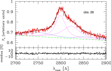
Figure 1. Exemplary SALT spectrum (last observation from 2018 December 11; red solid line) in arbitrary units, and decomposition into the underlying power law (dashed green line), Fe ii pseudo-continuum (blue dotted line), and two broad kinematic components modeling the shape of the Mg ii line (dotted magenta line). The total fit is shown as a solid black line.
Download figure:
Standard image High-resolution imageThe total equivalent width (EW) of the line was calculated from the fitted model, by integration in the 2700–2900 Å band. All four line components are included, i.e., two kinematic components, each with two doublet components. The EW of the line showed significant variations. The values of EW are listed in Table 1. We also calculated the EW of the Fe ii line in the spectral range 2700–2900 Å, and we also give these values in Table 1. The errors to EWs of Mg ii and Fe ii were determined by construction of the error contours and determining the appropriate limit for one parameter of interest (other parameters during the fitting were allowed to vary), and they represent 90% confidence level.
2.3. Photometry
The spectroscopic observations were supplemented with the photometric data from other instruments, whenever possible. High-quality photometry covering the first part of the observational campaign came from the OGLE-IV survey done with the 1.3 m Warsaw telescope at the Las Campanas Observatory, Chile. The exposures were done in the V band, with the exposure time of 240 s. These data have a typical error of 0.005 mag. The relative stability of this photometry for our source has been shown in Modzelewska et al. (2014).
At later epochs OGLE data were not available, but the spectroscopic observations by SALT were usually performed by supplementing photometry with SALTICAM, in g band. The exposure time was 45 s, and two exposures were usually done. The SALT/SALTICAM instrument is not suitable for high-quality photometry. Due to distortions of images taken by SALTICAM, a special, simple method for photometry has been developed. This method allows us to partially reduce the occurrence of significant changes in the number of counts for the background and objects depending on the position in the image. The measurement error is larger in this case than from OGLE, typically of order of 0.012. Since the two photometric sets were done using slightly different filters, we allowed for an arbitrary shift in the SALT photometry, and the amount of shift was optimized in the time span where the two measurements overlapped.
CTS C30.10 has also been observed between 2017 December 2 and 2018 April 1 employing the 40 cm Bohum Monitoring Telescope (BMT) located at the Universitätssternwarte Bochum, near Cerro Armazones in Chile (https://astro.ruhr-uni-bochum.de/Astrophysik/all_infos.html). The observations were carried out with the Johnson broadband filter Vj (λeff = 550 nm and zero mag flux f0 = 3836.3 Jy). Detailed information about the telescope, filters, and data reduction has been published in Ramolla et al. (2013). The light curve for this period of time is built by choosing 20 stars, bright enough and in proximity of the source as calibration stars, and the aperture used for the photometry is 3 75. The absolute photometric calibration is performed usually by comparison with the PANSTARSS Catalog. Since CTS C30.10 is not available in the PANSTARSS catalog, we used the conversion factor found for other objects that were observed with the same telescope, during the same nights. The photometry is given in Table 2.
Table 2. Photometric Observations of CTS C30.10 Performed with Various Instruments
| Start of the Observation | V | Error | Ref |
|---|---|---|---|
| 3597.75000 | 17.143 | 0.098 | 1 |
| 3627.71875 | 17.203 | 0.067 | 1 |
| 3667.70312 | 17.114 | 0.233 | 1 |
| 3676.64844 | 17.231 | 0.100 | 1 |
| 3692.68359 | 17.258 | 0.135 | 1 |
| 3714.64062 | 17.196 | 0.079 | 1 |
| 3733.61719 | 17.233 | 0.087 | 1 |
| 3756.59766 | 17.255 | 0.078 | 1 |
| 3819.46094 | 17.233 | 0.079 | 1 |
| 3863.35938 | 17.309 | 0.078 | 1 |
| 3980.78125 | 17.170 | 0.314 | 1 |
| 4003.71875 | 17.258 | 0.087 | 1 |
| 4013.71094 | 17.187 | 0.085 | 1 |
| 4032.71875 | 17.244 | 0.128 | 1 |
| 4049.66406 | 17.324 | 0.097 | 1 |
| 4062.56641 | 17.203 | 0.090 | 1 |
| 4079.61719 | 17.322 | 0.088 | 1 |
| 4108.54688 | 17.294 | 0.091 | 1 |
| 4119.54688 | 17.253 | 0.094 | 1 |
| 4129.52344 | 17.267 | 0.088 | 1 |
| 4174.48438 | 17.238 | 0.080 | 1 |
| 4351.78125 | 17.250 | 0.089 | 1 |
| 4394.68359 | 17.250 | 0.095 | 1 |
| 4414.72656 | 17.238 | 0.103 | 1 |
| 4442.62500 | 17.282 | 0.076 | 1 |
| 4467.62109 | 17.260 | 0.076 | 1 |
| 4503.46094 | 17.285 | 0.092 | 1 |
| 4530.50000 | 17.290 | 0.081 | 1 |
| 4721.73047 | 17.357 | 0.071 | 1 |
| 4756.25000 | 17.314 | 0.065 | 1 |
| 4775.72656 | 17.252 | 0.070 | 1 |
| 4793.65625 | 17.262 | 0.070 | 1 |
| 4808.56250 | 17.252 | 0.097 | 1 |
| 4823.05859 | 17.234 | 0.122 | 1 |
| 4855.57422 | 17.242 | 0.062 | 1 |
| 4868.47266 | 17.160 | 0.067 | 1 |
| 4894.48438 | 17.221 | 0.068 | 1 |
| 4916.41016 | 17.154 | 0.066 | 1 |
| 4939.39062 | 17.143 | 0.078 | 1 |
| 5104.71875 | 17.063 | 0.075 | 1 |
| 5121.71875 | 17.204 | 0.059 | 1 |
| 5151.66406 | 17.183 | 0.067 | 1 |
| 5188.60156 | 17.193 | 0.065 | 1 |
| 5223.53906 | 17.188 | 0.066 | 1 |
| 5269.43359 | 17.246 | 0.135 | 1 |
| 5302.38281 | 17.266 | 0.148 | 1 |
| 5495.71094 | 17.055 | 0.095 | 1 |
| 5544.60156 | 17.095 | 0.095 | 1 |
| 5561.61719 | 17.120 | 0.083 | 1 |
| 5590.55469 | 17.096 | 0.085 | 1 |
| 5618.52734 | 17.071 | 0.095 | 1 |
| 5653.43750 | 17.120 | 0.096 | 1 |
| 5820.76953 | 17.015 | 0.054 | 1 |
| 5867.62500 | 17.005 | 0.056 | 1 |
| 6199.79884 | 16.954 | 0.005 | 2 |
| 6210.81712 | 16.960 | 0.004 | 2 |
| 6226.67904 | 16.943 | 0.005 | 2 |
| 6246.69777 | 16.945 | 0.004 | 2 |
| 6257.74934 | 16.958 | 0.006 | 2 |
| 6268.68328 | 16.962 | 0.004 | 2 |
| 6277.68527 | 16.972 | 0.003 | 2 |
| 6286.66883 | 16.984 | 0.005 | 2 |
| 6297.61796 | 17.005 | 0.004 | 2 |
| 6307.57569 | 17.014 | 0.004 | 2 |
| 6317.64265 | 16.990 | 0.005 | 2 |
| 6330.65842 | 17.022 | 0.004 | 2 |
| 6351.54970 | 17.046 | 0.005 | 2 |
| 6363.57515 | 17.050 | 0.004 | 2 |
| 6379.48814 | 17.051 | 0.005 | 2 |
| 6379.49575 | 17.045 | 0.005 | 2 |
| 6387.51378 | 17.065 | 0.004 | 2 |
| 6637.67203 | 17.154 | 0.004 | 2 |
| 6651.62307 | 17.163 | 0.004 | 2 |
| 6665.60641 | 17.167 | 0.004 | 2 |
| 6678.60051 | 17.159 | 0.004 | 2 |
| 6689.67477 | 17.136 | 0.004 | 2 |
| 6700.63830 | 17.145 | 0.006 | 2 |
| 6715.57763 | 17.117 | 0.004 | 2 |
| 6740.49251 | 17.102 | 0.004 | 2 |
| 7013.64000 | 17.016 | 0.012 | 3 |
| 7036.65430 | 17.024 | 0.004 | 2 |
| 7048.65618 | 17.021 | 0.004 | 2 |
| 7060.60707 | 17.031 | 0.005 | 2 |
| 7084.53744 | 17.052 | 0.005 | 2 |
| 7110.91000 | 17.064 | 0.013 | 3 |
| 7118.50958 | 17.055 | 0.005 | 2 |
| 7240.35000 | 17.058 | 0.012 | 3 |
| 7253.89503 | 17.058 | 0.004 | 2 |
| 7261.88618 | 17.020 | 0.004 | 2 |
| 7267.91792 | 17.021 | 0.005 | 2 |
| 7273.85028 | 17.058 | 0.004 | 2 |
| 7295.84577 | 17.052 | 0.005 | 2 |
| 7306.78400 | 17.082 | 0.004 | 2 |
| 7317.74327 | 17.101 | 0.005 | 2 |
| 7327.77769 | 17.109 | 0.005 | 2 |
| 7340.70964 | 17.126 | 0.004 | 2 |
| 7342.33000 | 17.132 | 0.012 | 3 |
| 7355.69767 | 17.119 | 0.005 | 2 |
| 7363.66962 | 17.109 | 0.004 | 2 |
| 7374.71221 | 17.138 | 0.004 | 2 |
| 7385.56062 | 17.154 | 0.004 | 2 |
| 7398.62071 | 17.145 | 0.004 | 2 |
| 7415.58887 | 17.149 | 0.004 | 2 |
| 7421.90000 | 17.113 | 0.012 | 3 |
| 7426.56982 | 17.135 | 0.004 | 2 |
| 7436.52896 | 17.123 | 0.005 | 2 |
| 7447.53110 | 17.115 | 0.004 | 2 |
| 7457.52592 | 17.140 | 0.004 | 2 |
| 7664.25000 | 17.127 | 0.012 | 3 |
| 7687.22000 | 17.107 | 0.012 | 3 |
| 7717.70845 | 17.106 | 0.004 | 2 |
| 7805.10000 | 17.075 | 0.012 | 3 |
| 7965.86000 | 17.125 | 0.011 | 3 |
| 7973.90556 | 17.181 | 0.008 | 4 |
| 7973.91644 | 17.188 | 0.010 | 4 |
| 8038.86464 | 17.155 | 0.006 | 4 |
| 8040.47000 | 17.171 | 0.012 | 3 |
| 8091.20000 | 17.153 | 0.006 | 4 |
| 8097.30000 | 17.125 | 0.006 | 4 |
| 8099.30000 | 17.127 | 0.004 | 4 |
| 8099.38000 | 17.153 | 0.012 | 3 |
| 8128.20000 | 17.106 | 0.006 | 4 |
| 8135.10000 | 17.102 | 0.006 | 4 |
| 8142.10000 | 17.123 | 0.004 | 4 |
| 8166.00000 | 17.097 | 0.006 | 4 |
| 8174.00000 | 17.104 | 0.008 | 4 |
| 8181.00000 | 17.110 | 0.008 | 4 |
| 8197.00000 | 17.080 | 0.010 | 4 |
| 8206.00000 | 17.082 | 0.008 | 4 |
| 8211.00000 | 17.059 | 0.009 | 4 |
| 8368.40000 | 17.043 | 0.004 | 4 |
| 8374.40000 | 17.033 | 0.012 | 3 |
| 8415.30000 | 17.020 | 0.005 | 4 |
| 8433.05000 | 17.020 | 0.012 | 3 |
| 8462.65000 | 16.995 | 0.011 | 3 |
| 8152.55 | 17.079 | 0.02 | 5 |
| 8159.55 | 17.070 | 0.02 | 5 |
| 8166.54 | 17.090 | 0.02 | 5 |
| 8173.53 | 17.008 | 0.02 | 5 |
| 8180.5 | 17.087 | 0.02 | 5 |
| 8187.52 | 17.097 | 0.02 | 5 |
| 8194.49 | 17.039 | 0.02 | 5 |
| 8202.49 | 17.031 | 0.02 | 5 |
| 8209.5 | 17.065 | 0.02 | 5 |
| 8216.49 | 17.074 | 0.02 | 5 |
| 8223.47 | 17.102 | 0.02 | 5 |
Note. References: (1) CATALINA survey; (2) OGLE photometry; (3) SALTICAM SALT photometry; (4) BMT; (5) SMART (not included in time delay computations).
A machine-readable version of the table is available.
Having the photometric coverage of the monitored period, we obtained the photometric light curve. The Mg ii light curve was also obtained with the use of photometry since SALT spectra are not spectrophotometric measurements owing to the construction of the telescope. Having the photometric light curve in V band, we used either SALTICAM measurement or linear interpolation between the nearest available photometric points to obtain the continuum flux at the date of the spectroscopic observation. We corrected the flux for absorption in our Galaxy taken from NED. This allowed us to calibrate the power-law component in our model and to derive the continuum flux value at 2800 Å rest frame. We then calculated the line flux and errors using the numerically determined value of the EW and its error. We integrated the model, not the data, but all four Mg ii components were included (see Section 2.2). Such an Mg ii light curve was ready for further analysis, including time delay measurements. The normalized dispersion of the continuum in the whole period is 6.0%, and the line flux variability, if we neglect observation 6, is at the level of 5.2%, lower (but not much) than the variability amplitude of the continuum.
In the period of 2018 February 3–April 14 we also performed dense photometric observations of CTS C30.10 with the use of the 1.3 m SMART telescope at the Cerro Tololo Inter-American Observatory. Observations were performed three times per night, roughly every week, with an exposure time of 60 s. Photometry from these data was prepared using IRAF daophot software and was typically of accuracy of 0.02, which is lower than what was achieved with other instruments, so we finally used these data only to constrain the variability properties of the quasar in the Appendix.
3. Spectral Properties in the Mg ii Line Region
Since the Mg ii line fitting in CTS C30.10 requires two broad kinematic components, we first analyze the variability in the spectral shape of the line reflected directly in the line fitting. In Figure 2 we show the time dependence of the ratio of the second Lorentzian kinematic component to the total line.
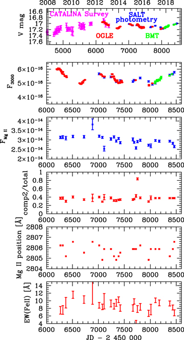
Figure 2. From top to bottom, photometric light curve of CTS C30.10 from three instruments, flux at 3000 Å in erg s−1 cm−2 Å−1, Mg ii line flux in erg s−1 cm−2, the ratio of the second kinematic component of the line to the total line flux, the mean position of the line (defined as wavelength where half of the total integrated line luminosity is contained; see Section 3), and the EW of the Fe ii pseudo-continuum measured between 2700 and 2900 Å. There is one clear outlier with large error bars in the line flux plot (observation 6 when the weather conditions were not very good) and one outlier in the component ratio plot (observation 18; see Figure 3).
Download figure:
Standard image High-resolution imageOne of the points, corresponding to observation 18, is a strong outlier, with the second component strongly dominating. The value of the χ2 in this fit is particularly high, but we were not able to find another fit, with a typical value of the component ratio. The overall spectrum in this observation (see Figure 3) is not very different from the representative spectrum (see Figure 1), but there seems to be a trace of absorption close to the peak of the line, which leads to such an atypical spectral fit. Apart from observation 18, the mean FWHM of the first component is 2780 km s−1, and the second component is slightly broader, with a mean FWHM of 3884 km s−1. The corresponding dispersion values measured in our observations are 320 and 530 km s−1, and the typical accuracy of the width determination in individual observations is usually better, about 200 and 300 km s−1, but in some data sets errors are larger and they contribute to the overall dispersion.
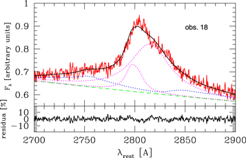
Figure 3. SALT spectrum (observation 18, 2016 December 29) that shows the atypical ratio of the two kinematic components of the Mg ii line seen as a strong outlier in Figure 2. See Figure 1 for the description of spectra decomposition.
Download figure:
Standard image High-resolution imageWe check whether the role of the two kinematic components varies with time, and to this aim we plot the ratio of the flux contained in the second component to the total line flux (see Figure 2). There is an overall weak rising trend in the ratio. The linear fit to this trend gives a systematic change in the ratio of (1.83 ± 0.63) × 10−5 yr−1 (1σ error). This might be related to the fact that we fixed the redshift of the first kinematic component, and if there is a systematic change in the Mg ii line position as a whole line, it would show this behavior. Line shifts in quasars are a general phenomenon observed in high-quality data (see, e.g., Średzińska et al. 2017). We thus test the line position in the data, by subtracting from the total flux the fitted continua (power law and Fe ii) and integrating the line flux over the wavelength up to a wavelength value where half of the total line luminosity is contained. This method is less sensitive to the accuracy of the peak determination of the line and seems more appropriate for an asymmetric line. The resulting line position is shown in Figure 2, but a linear fit to this trend shows that the line systematic shift is not significant, (8.2 ± 28.9) × 10−5 Å yr−1. This is orders of magnitude lower than the fast displacement observed in another of the quasars studies with SALT (0.64 ± 0.11 Å yr−1, in HE 0435-4312; Średzińska et al. 2017). We need to extend our monitoring to decide whether we observe a systematic line drift or just a change in the line shape since the effect is so weak.
3.1. Mean and rms Spectrum
Since no obvious systematic drift is seen in the Mg ii line, we calculate the mean and the rms variation of the Mg ii line. For that purpose, we normalize each of the SALT spectra using the photometry provided in Table 2. We had to remove observation 6 from the composite plot since these data are particularly noisy, the flux varied up to a factor of 2 between the consecutive wavelength bins, and that considerably affected the mean and rms. This observation was performed in the presence of some thin clouds. The remaining spectra are of much higher quality.
The mean spectrum traces the general shape of the Mg ii line very nicely, with very low noise (see Figure 4). The two-component character of the line shape is well seen. The mean spectrum is well fitted by the same model; there are some departures between the data and the model in the Fe ii region, but other Fe ii templates do not provide a better fit. A comparable (but slightly worse) fit was achieved by the Fe ii template d11-m20-21-735 with lower number density (1011 cm−3) but higher ionizing flux. Using the mean spectrum decomposition, we measured the total FWHM of the Mg ii line, treated as a single-component asymmetric line. The obtained value, 5009 ± 325 km s−1, locates CTS C30.10 among type B quasars in classification by Sulentic et al. (2000). Since the total line FWHM is not a parameter directly fitted to the data (for those parameters we have errors from the contour error plots), we determined the total FWHM line width from the four-component line model (see Section 2.2), and uncertainties were estimated interpolating a total profile at ±5% with respect to the half-maximum of the profile, which takes into account the possible asymmetries in the total profile. That percentage is appropriate for the high S/N (∼320) of the mean spectrum.
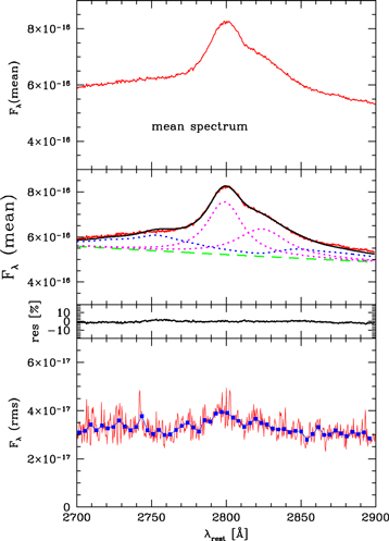
Figure 4. Mean (top panel) spectrum, its decomposition (middle panel), and rms spectrum (bottom panel) of CTS C30.10, calculated without observation 6. Flux given in units of erg s−1 cm−2 Å−1.
Download figure:
Standard image High-resolution imageWe removed the observation 6 spectrum only in the mean and rms computations. Apart from that, this observation, despite a relatively high noise level, gave a meaningful value for the line flux (but with large error; see Figure 2) and was used in further considerations.
4. Time Delay Measurements of Mg ii Line
The number of spectra collected by us with the SALT telescope (26) just matches the minimum (25 spectra) necessary to obtain a viable estimate of the Mg ii time delay (Czerny et al. 2013). Therefore, we use six different methods to obtain reliable results. The first method is the classical interpolated cross-correlation function (ICCF) method, most popular in AGN monitoring (e.g., Gaskell & Peterson 1987; Peterson et al. 2004). Edelson et al. (2019) argued that this method brings the most reliable results despite giving relatively large errors. Next, we use the discreet correlation function (DCF) and z-transformed DCF. The fourth method is based on the damped random walk (DRW) model of the quasar variability (Kelly et al. 2009), and it was developed into the software JAVELIN (Zu et al. 2011, 2013, 2016). We also use the method based on curve shifting and χ2 fitting, which was also used by several authors (e.g., Kundić et al. 1997; Czerny et al. 2013). Finally, we use the von Neumann estimator.
4.1. ICCF
Constructing ICCF is the traditionally used method of calculating the time delay in reverberation mapping of AGNs (Peterson et al. 2004). We mostly followed this general approach. However, we do not supplement the data curves with extrapolation when photometry or spectroscopy cannot be obtained through interpolation. Peterson et al. (2004) argue that the extrapolation decreases the error, but our light curves, particularly the spectroscopic one, are so short (only 26 measurements) that introducing not fully justified points may strongly bias the results. Otherwise, we perform the computations in the standard way, subtracting the mean and normalizing the light curves by the variance, but at that stage we use the measurement errors, so our mean and variance are calculated as a weighted quantities. We think that this is important since the errors in our data are not always similar to the typical error.
The best delay from ICCF is determined by the fit of the centroid to the values above 0.8 of the peak values. As a basic output, we treat the solution obtained as a sum of two options: either photometric points are interpolated to match shifted spectroscopic points, or the spectroscopic points are interpolated to match the shifted photometric points. This method is recommended by Peterson et al. (2004). However, we also use each of the two methods mentioned above separately, and they lead to strongly different results, shown in Figure 5 and in Table 3. The asymmetric method, with the interpolation of spectroscopic points, leads to high ICCF cross-correlation values, ∼0.92, close to the peak, implying a time delay of 542 days. On the other hand, interpolation of the photometric points shows a much lower level of correlation, at most ∼0.51, and the highest peak appears at 1073 days and strongly dominates the other peaks. Thus, high values of the ICCF in the previous case simply result from very few spectroscopic points being interpolated to dense photometric coverage that carries redundant information. Symmetrization points toward the lower value of the lag. There is also a clear second peak at 1070 days in the observed frame, but the ICCF peak is slightly lower. Thus, the result from ICCF is not unique, and this problem appears occasionally in reverberation measurements (see, e.g., Du et al. 2016). However, taking into consideration that we use 133 photometric points and 26 spectroscopic points, it is not clear that averaging is more reliable than interpolating only the denser (photometric) light curve. This would favor the longer value of the time delay, just above 1000 days. There is also a third peak, at 1300 days, and its height and position are similar in all three approaches.
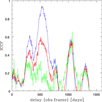
Figure 5. ICCF calculated by interpolating only photometry (green line), that calculated by interpolating only spectroscopy (blue line), and the averaged symmetric result (red line).
Download figure:
Standard image High-resolution imageTo obtain the error on the measured time delay, we use the model-independent method based on the bootstrap approach, as described in detail in Peterson et al. (1998). The uncertainties are large. For quoting the bootstrap best value delay and its error, we use the whole histogram, including multiple peaks. Large errors and the sensitivity of the results to the method are due to the fact that the distribution is not a single peak distribution, as clearly seen in Figure 5 from the ICCF distribution, and the same shows up in the histograms obtained through simulations when using the bootstrap method.
Finally, we also tested the sensitivity of the results to the few spectroscopic points of likely lower quality. As a test, we removed observations 6, 9, and 17. All of them are clear outliers in Figure 2, the third panel (the first two cases) and the bottom panel (the last one, showing an apparent problem with Fe ii fitting in these data). The results are also included in Table 3. The results are qualitatively the same as before.
Table 3. Measured Delays for the Mg ii Line in CTS C30.10 from Various Methods in Observed Frame
| Method | τ |
|---|---|
| (days) | |
| ICCF symmetric |

|
| ICCF interp.phot. |

|
| ICCF interp.spectr. |

|
| ICCF symmetric (−3 points) |

|
| ICCF interp.phot. (−3 points) |

|
| ICCF interp.spectr. (−3 points) |

|
| DCF (−3 points) | 1066 ± 64 |
| zDCF (without Catalina) |

|
| JAVELIN all points |

|
| JAVELIN (−2 points) |

|
| JAVELIN all points (bootstrap) |

|
| χ2 symmetric |

|
| χ2 interp.phot. |

|
| χ2 interp.spectr. |

|
| χ2 symmetric (−3 points) |

|
| χ2 interp.phot. (−3 points) |

|
| χ2 interp.spectr. (−3 points) |

|
| VN | 948+90−90 |
Download table as: ASCIITypeset image
4.2. DCF
Since linear interpolation between points does not fully represent the variability of the source between the measured points, the DCF, which does not require such interpolation, has been proposed in the time delay measurement context by Edelson & Krolik (1988). We thus used this approach as well, removing the same three outliers as before, i.e., observations 6, 9, and 17. We also excluded the more noisy CATALINA survey data from the photometry light curve. The resulting plot for the DCF value as a function of the time lag is shown in Figure 6, where we considered the time lag binning of 100 days. In fact, the DCF method depends quite strongly on a time lag binning. Since the mean time between observations for the continuum and line-emission light curve is Δtcont = Tcont/(nobs − 1) = 28.4 days and Δtline = 99.8 days, respectively, the time lag bin should be at least equal to the larger of the two timescales; hence, we set Δτ = 100 days. Again, we see four peaks, at ∼250 days (DCF ∼ 0.47), ∼450 days (DCF ∼ 0.51), ∼850 (DCF ∼ 0.50), and ∼1050 days (DCF ∼ 0.59), the last being the dominant one. This is consistent with the previous analysis using the ICCF.
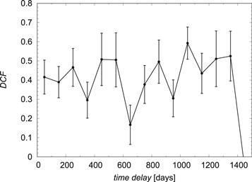
Figure 6. DCF value with its uncertainties as a function of the time lag in days. The time lag bins are 100 days. Lag is measured in days in observed frame.
Download figure:
Standard image High-resolution imageNext, we focused on the surroundings of the dominant peak at ∼1050 days within the time range of (900, 1200) days and a time step of 40 days. The result is plotted in Figure 7, where the peak is at τ ∼ 1069 days (DCF ∼ 0.71). We estimate the uncertainty of the dominant peak by fitting the Gaussian function to the data in Figure 7, by which we obtain the mean estimate and the symmetric 1σ error of τDCF = 1066 ± 64 days.
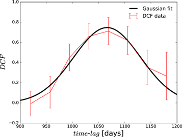
Figure 7. DCF value with its uncertainties as a function of the time lag in days around the dominant peak at 1069 days. The time lag bins are 40 days. The black solid line represents the Gaussian fit to determine 1σ uncertainties.
Download figure:
Standard image High-resolution image4.3. zDCF
Alexander (1997) introduced the z-transformation of the discrete correlation function (zDCF) to correct several biases of the DCF (see Edelson & Krolik 1988) by making use of the equal population binning and Fisher's z-transform.9
In the following analysis, we removed 54 points from the continuum light curve, which corresponded to the CATALINA survey with larger observational errors. In the end, we had 82 continuum points and 26 line-emission points. The calculated zDCF values versus the time lag including the uncertainties are shown in Figure 8. Next, we focused on the largest zDCF peak between 800 and 1400 days in Figure 8. We applied the maximum likelihood function of Alexander (1997) to determine the zDCF peak and its uncertainties, and we obtained  days.
days.
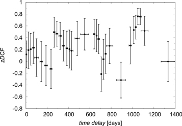
Figure 8. Calculated zDCF values vs. the time lag in days, in the observed frame, including the uncertainties for both the time lag and the zDCF value.
Download figure:
Standard image High-resolution image4.4. JAVELIN
To measure the time lag between the continuum emission and the line's response, we also use the JAVELIN10 software (Zu et al. 2011, 2013, 2016). It models the continuum light curve as a stochastic process, here the DRW (Kelly et al. 2009; Kozłowski et al. 2010; MacLeod et al. 2010), and assumes that the light curves of the emission line are the lagged, smoothed, and scaled versions of the continuum light curve. The Markov chain Monte Carlo (MCMC) posterior probabilities produced by JAVELIN include such parameters as the two DRW model parameters (the variability timescale and amplitude), the time lag, the smoothing width of the top-hat function, and the amplitude scale factor of the emission line to the continuum (Aline/Aphoto).
In Figure 9, we present the posterior probability distribution in the lag–Aline/Aphoto plane. Several probability maxima are readily visible, of which the one at 1068 days is the strongest. A by-eye inspection of the line light curve uncovered two plausible outliers at JD = 2,456,886.5 and 2,457,110.5. We considered two cases here, where the line data were modeled in full (top panel of Figure 9) and with the two outliers removed (bottom panel of Figure 9). The best-measured observed-frame time lags obtained from the strongest peak are  days for the full-line light curve and
  days for the cleaned light curve, where the error bars are asymmetric 1σ uncertainties. The rest-frame lags are then, respectively,
  days and
  days, fully consistent with each other.
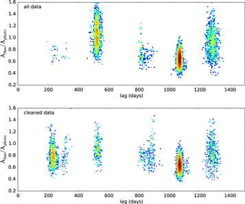
Figure 9. Posterior probability distributions in the observed frame obtained from the JAVELIN software for the full data (top) and cleaned line data (bottom). The strongest probability in both cases appears to be at the lag of 1068 days, which corresponds to 562 days in the rest frame.
Download figure:
Standard image High-resolution imageIn order to understand the probability structures in Figure 9, we performed simulations of 100 light-curve pairs for (1) the input time lag of 1000 days and (2) the input time lag of 500 days. We used the DRW model with the typical input AGN variability parameters, the timescale of 1 yr, and the asymptotic variability of 0.25 mag (Kozłowski 2016). The cadence and photometric noise were set to be identical to the real data. Then, we modeled the simulated data with JAVELIN in the same fashion as the real data, including the cadence and the error bars.
We find that for the simulations with the lag of 1000 days, 10 cases (10%) show incorrect measurements, other than the input 1000 days. In 25 (25%) cases we also find secondary probability peaks in the vicinity of 500 days (similar to what is observed in real data), in 44 cases (44%) probability peaks at 1200–1300 days, in 27 cases (27%) peaks at about 800 days, and in 22 cases (22%) peaks at about 200 days. Generally, the probability structures in the simulated data resemble quite well what we observe in the real data, and the additional peaks to the main one at 1000 days are expected based on simulations (even if there is a single lag present in the data).
Analysis of simulations with the 500-day lag returns only 2 cases (2%) with peaks in the vicinity of 1000 days, as well as41 cases (41%) at about 1200 days. General inspection of the output appears to be different than for the real data and simulations with the input lag of 1000 days.
JAVELIN-claimed errors are usually very small since the software focuses on the error determination of the position of the most significant peak. In order to make JAVELIN errors comparable to other measurement errors, we performed the bootstrap approach, calling JAVELIN software for 100 bootstrap-generated curves, and at the end we performed the search for the best solution and its error using the whole distribution of time delays instead of focusing on the strongest peak. Now the error is much larger, giving  days in the observed frame. The error is still smaller than in ICCF but larger than in zDCF. For completeness, we quote this value in Table 3, marked as bootstrap.
4.5. χ2 Method
This method is frequently used in quasar lensing studies, and Czerny et al. (2013) found that it works better than ICCF for the red-noise AGN variability. Thus, we also apply this method. The light curves are again prepared as for ICCF, by subtracting the mean and renormalizing by variance. Then, the photometric or spectroscopic light curve is shifted with respect to the other one, and, as for ICCF, we can use the asymmetric approach (interpolating only photometry, or interpolating only spectroscopic light curve), or we can use both and average the results. We use only the linear interpolation, as in ICCF. We estimate the similarity of the shifted curves by simply calculating the χ2 value. Thus, the minimum of the χ2 indicates the most likely time delay. The results are shown in Figure 10. The minimum is always at the location indicated by the JAVELIN method (see Section 4.4).
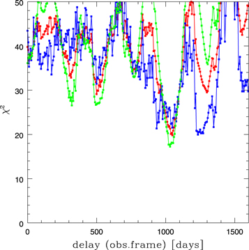
Figure 10. χ2 distribution, color-coded as in Figure 5, with minima implying the best solution for time delay.
Download figure:
Standard image High-resolution imageWe assign the error again by performing Monte Carlo simulations as in Section 4.1. The error bars given in Table 3 are much larger than in the standard case of the JAVELIN method, comparable to ICCF. However, the distribution is more concentrated around the best solution, without an extended tail as in the ICCF method. What is more important, the resulting most probable time delay is the same, independently from the choice of the data set for interpolation.
Also in this case we tested the sensitivity or the removal of the outlying spectroscopic points. We removed again SALT observations 6, 9, and 17. The results for the best value of the time delay in this case did not change (see Table 3), so the method seems quite stable.
4.6. Von Neumann Estimator
Finally, we complement the previous ways of time delay determination by the method of randomness measure or the complexity measure of the data. This method has the advantage that it does not require either the interpolation of data, as for the ICCF method, or the binning in the correlation space, and it is largely model independent. The measures of the randomness or the complexity of the data are based on different kinds of estimators, among which the optimized von Neumann's scheme turns out to be most robust (Chelouche et al. 2017). The von Neumann (VN) estimator of the randomness (or regularity) of data is defined as the mean-square successive difference,
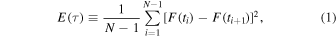
where  is the combined continuum and time-delayed line light curve. When the searched time delay τ is close to the actual time delay between the light curves, τ ≃ τ0, the VN estimator reaches the minimum. We applied the optimized scheme of the VN estimator based on the python script of Chelouche et al. (2017).11
We show the dependence of the VN estimator on time delay in Figure 11. In the search interval [0, Tmax] = [0, 1300] days, there are three distinct minima, with the global one at τ0 ≃ 945 days, followed by τ' = 239 days and τ'' = 573 days. In the further analysis, we assume that the time delay τ0 ≃ 945 stands for the actual time delay, but this needs to be evaluated further statistically.
is the combined continuum and time-delayed line light curve. When the searched time delay τ is close to the actual time delay between the light curves, τ ≃ τ0, the VN estimator reaches the minimum. We applied the optimized scheme of the VN estimator based on the python script of Chelouche et al. (2017).11
We show the dependence of the VN estimator on time delay in Figure 11. In the search interval [0, Tmax] = [0, 1300] days, there are three distinct minima, with the global one at τ0 ≃ 945 days, followed by τ' = 239 days and τ'' = 573 days. In the further analysis, we assume that the time delay τ0 ≃ 945 stands for the actual time delay, but this needs to be evaluated further statistically.
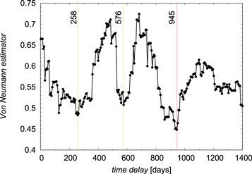
Figure 11. Dependence of the value of VN estimator on the time delay in days in the observed frame.
Download figure:
Standard image High-resolution imageTo determine the uncertainty of  , we perform bootstrapping by generating subsamples of 10,000 continuum and line-emission light curves based on the actual observed light curves. This way we obtain a distribution of the time delay around the global minimum; see Figure 12. The distribution is broad, with a mean and standard deviation of
  days, which is consistent within the uncertainty with the previously determined time delays via the JAVELIN and χ2 methods, further strengthening the time delay of ∼1000 days. The advantage of the optimized VN method is that no stochastic model and assumption of quasar variability are needed.
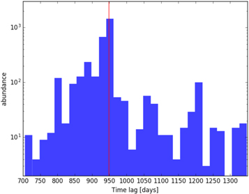
Figure 12. Distribution of the time delay as determined by the VN estimator for 10,000 light curves generated by bootstrapping from the original observed pair of light curves. The red vertical line represents the mean value of 952 days in the observed frame.
Download figure:
Standard image High-resolution image4.7. Best Determination of the Time Delay
The quality of our data is not good enough to give always the same result, independently of the method. Three candidate time delay values appear: one around 1070 days, one at 550 days, and one at 1250 days in the observed frame. JAVELIN gives the smallest errors, and this method favors the intermediate delay, with or without three outliers removed.
The results from various methods are not easy to compare since error determination is very sensitive to the method used. JAVELIN returns the error of the best solution position, while in other methods the errors are based on the whole statistics, including side peaks as well. This basically explains the huge difference in errors between JAVELIN and χ2, ICCF and VN. If we force JAVELIN to use the same approach as the other methods do (see Section 4.4), the errors from JAVELIN are still somewhat smaller than from ICCF, comparable to χ2 results, but larger than the errors from zDCF and VN. Still, the value of the best time delay in JAVELIN seems very insensitive to the details like removal (or not) of outliers and the way errors are measured.
In the case of the ICCF and χ2 methods, the delay can be determined using either a symmetric approach to photometry and spectroscopy or an asymmetric one. Since the photometric coverage is much better, actually the asymmetric method requiring interpolation only for photometric data seems more justified.
Thus, we calculated the weighted average value of the best time delay by including only the full data ICCF and χ2 for photometric interpolation and the results from the other three methods. For JAVELIN, we used the standard result. Such an average value is 1068 days in the observed frame, not far from the JAVELIN result itself.
A delay of that order seems to be most consistent with the visual impression of the data. In Figure 13 we show the continuum and the line light curves, average-subtracted and renormalized by variance, with photometric curve shifted by a few trial values of the time delay. The middle one represents best the overall pattern. This additionally supports the adoption of the mean value calculated above.
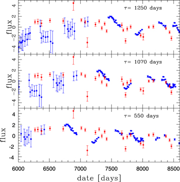
Figure 13. Continuum (blue points) and Mg ii flux (red points) after subtracting the average and renormalization by the corresponding variance plotted for three cases of the time lag by shifting the photometric data.
Download figure:
Standard image High-resolution imageHowever, such an averaging is not statistically viable (although informative), and determination of the error of this quantity is even more problematic. The bootstrap approach in the case of ICCF gives values that seem too high, and the bootstrap approach to χ2 indicates delays in the range from 939 to 1281 days. Such an error is large, but in our opinion this is the most realistic and conservative approach. Simulations of the ICCF and χ2 results with the method of Timmer & Koenig (1995) (see the Appendix) give errors of order of 30–60 days, but they do not include the information about the light-curve properties, apart from the power density spectrum (PDS). So finally we adopt, as the best time delay, the value of 1068 days, and for the error we adopt the limits from the χ2 bootstrap, i.e.,  , in the observed frame. JAVELIN small error results are well within these limits.
4.8. Black Hole Mass in CTS C30.10
Determination of the time delay opens the way to estimation of the black hole mass. Our rms spectrum is not of high quality, but the mean spectrum can be used for that purpose. Black hole mass can be measured as

or
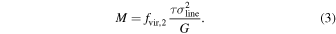
We have measured the FWHM values and the line dispersion σline from the fitted mean profile. The corresponding values are 5009 and 3326 km s−1. The ratio of FWHM/σline is 1.51. For the virial factor, fvir, we use the recommendation of Collin et al. (2006): factor of 1.43 in the first case and factor of 3.85 in the second case. The two expressions above give the two values of the black hole mass: 3.9 × 10⁹ M⊙ and 4.6 × 10⁹ M⊙. The second method is generally recommended by Collin et al. (2006), and it compares well with the black hole mass of 4.9 × 10⁹ M⊙ favored by Modzelewska et al. (2014) for this source.
Table 4. Measured Delays for the Mg ii Line
| Object | z | Tau | Err+ | Err− |

|
Err | Reference Tau | Reference L |
|---|---|---|---|---|---|---|---|---|
| Rest Frame | ||||||||
| 141214.20 + 532546.7 | 0.45810 | 36.7 | 10.4 | 4.8 | 44.63882 | 0.00043 | Shen et al. (2016) | Shen et al. (2018) |
| 141018.04 + 532937.5 | 0.46960 | 32.3 | 12.9 | 5.3 | 43.72880 | 0.00506 | Shen et al. (2016) | Shen et al. (2018) |
| 141417.13 + 515722.6 | 0.60370 | 29.1 | 3.6 | 8.8 | 43.68735 | 0.00290 | Shen et al. (2016) | Shen et al. (2018) |
| 142049.28 + 521053.3 | 0.75100 | 34.0 | 6.7 | 12.0 | 44.69091 | 0.00090 | Shen et al. (2016) | Shen et al. (2018) |
| 141650.93 + 535157.0 | 0.52660 | 25.1 | 2.0 | 2.6 | 43.77781 | 0.00198 | Shen et al. (2016) | Shen et al. (2018) |
| 141644.17 + 532556.1 | 0.42530 | 17.2 | 2.7 | 2.7 | 43.94795 | 0.00105 | Shen et al. (2016) | Shen et al. (2018) |
| CTS 252 | 1.89000 | 190.0 | 59.0 | 114.0 | 46.79373 | 0.09142 | Lira et al. (2018) | NED NUV GALEX |
| NGC 4151 | 0.00332 | 6.8 | 1.7 | 2.1 | 42.83219 | 0.18206 | Metzroth et al. (2006) | Code & Welch (1982) |
| NGC 4151 | 0.00332 | 5.3 | 1.9 | 1.8 | 42.83219 | 0.18206 | Metzroth et al. (2006) | Code & Welch (1982) |
| CTS C30.10 | 0.90052 | 564.0 | 109 | 71 | 46.023a | 0.026 | this paper | this paper |
Note.
aObtained from the mean V mag 17.1, for the cosmology H0 = 70 km s−1 Mpc−1, Ωm = 0.3, ΩΛ = 0.7 (Kozłowski 2015).Download table as: ASCIITypeset image
4.9. Radius–Luminosity Relation for Mg ii Line
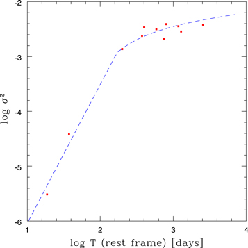
We now combine the measurements available in the literature (see Section 1) with our measurement of the time delay in CTS C30.10. The list of the measurements is given in Table 4, and the plot using the final value set in Section 4.7 is shown in Figure 14. We use these data to determine the R–L relation for the Mg ii line. The best fit, taking into account errors in both axes, reads as

and it is shown in Figure 14 with a solid line. There is some dispersion in the plot. CTS C30.10 is much brighter than AGNs measured by Shen et al. (2016). On the other hand, it is somewhat less luminous and located at lower redshift than CTS 252, but our time delay is longer than for CTS 252. The black hole mass in CTS 252 is 1.26 × 10⁹ M⊙, lower than the most probable mass in CTS C30.10, while the luminosity is higher by a factor of 5. The FWHM of the Mg ii line is also much narrower in CTS 252 (3800 km s−1) than the total FWHM of the line in CTS C30.10 (5009 ± 325 km s−1). This strongly suggests that the Eddington ratio in these two objects is different, much lower in CTS C30.10 than in CTS 252. Thus, the difference in the detected lag may be related to the difference in the Eddington ratios, in a similar way to how it is for Hβ line lags, with considerable lag shortening (for a given monochromatic luminosity) with the rise of the Eddington ratio (Du et al. 2016; M. L. Martinez Aldama 2019, in preparation).
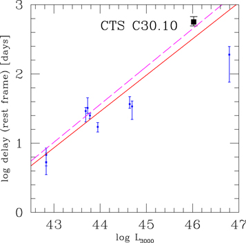
Figure 14. Radius–luminosity relation for Mg ii line (points and errors given in Table 4). The solid red line is the best fit for all the data points. The long-dashed magenta line comes from Bentz et al. (2013) for the Hβ line (model Clean2) under the assumption that L3000 = 1.84L5100.
Download figure:
Standard image High-resolution imageAs a reference, we plot in Figure 14 the radius–luminosity relation of Bentz et al. (2013), their model Clean2. Since now we use L3000 on the x-axis, we transformed the relation by recomputing L3000 from L5100 using the ratio of the bolometric corrections derived by Richards et al. (2006): L3000 = (10.33/5.62)L5100. Both relations have the same slope within the error (slope of the Bentz et al. 2013 relation is 0.546 ± 0.027), and the normalization is also similar.
Our result shows that the Mg ii line kinematically is very similar to the Hβ line. In their recent work Popović et al. (2019) came to a different conclusion on the basis of the line shape study in 284 sources, stressing the difference in the line wings, as noticed also before by Trakhtenbrot & Netzer (2012). However, this difference was mostly seen for lines with FWHM above 6000 km s−1. CTS C30.10 and all of the sources in Table 4, apart perhaps from NGC 4151 (FWHM = 6558 ± 1880 km s−1; Metzroth et al. 2006), have narrower Mg ii lines, between 2391 and 4066 km s−1 in the Shen et al. (2016) sample.
5. Discussion
Using our spectroscopic observations from our 6 yr campaign performed with the SALT telescope and supplemented with photometry, we were able to determine the time delay of the Mg ii line in CTS C30.10. Our result complements the delays measured for lower-redshift, lower-luminosity sources.
We used six different methods to measure the time delay, and the JAVELIN method gave the best estimate, with the smallest error. A conservative error estimate, based on all methods, gives much a larger error, but the JAVELIN small error determination is well within the broader boundaries that we adopted in further study. However, it is interesting that apart from the strongly favored time delay just above 1000 days, there are traces of the secondary solutions at ∼500 days, which even dominated in results from the ICCF. Simulations based on the PDS discussed in the Appendix did not show such secondary peaks, but they were present in the JAVELIN approach and in all bootstrap results. The presence of the secondary peak does not necessarily mean that there is more than one timescale in the process, but it might suggest that the transfer function is more complex than a simple Gaussian smearing adopted in Timmer & Koenig (1995) simulations. The quality of our data is not good enough to test, if it is a signature of the broader range of timescales present in the system. For example, the time delay for two separate kinematic components may not be the same, but we need more data points to test that.
Our measurement, combined with the previous results, shows that the Mg ii line time delay forms a similar pattern to the Hβ radius–luminosity (R–L) relation. The measured sources do not all follow Bentz et al. (2013), but the same is seen in new measurements (Du et al. 2016; Grier et al. 2017), where the initially indicated R–L gave the maximum time delay for a given monochromatic luminosity bin. The slope of the R–L relation is consistent within the error with the slope of Bentz et al. (2013). The Mg ii line seems to be somewhat shifted (by some ∼10%–20%) toward shorter delays, but we included all sources in our analysis, while Bentz et al. (2013) fit only the low Eddington ratio objects, as implied by new measurements (Du et al. 2016; Grier et al. 2017). This natural selection happened since high Eddington ratio sources are in general less variable in the optical/UV band (Zhou et al. 2006; Ai et al. 2010) and thus are less likely to be selected for systematic monitoring. In addition, with uncertain scaling between L3000 and L5100 we cannot give an accurate value for this shift. Wang et al. (2009) found that on average Mg ii lines are narrower by some 15% than Hβ lines, which would imply an expected shift in the R–L by ∼25% toward longer delays. Thus, we consider such trends as overall consistent with our finding. Similar shifts in black hole mass determination from Hβ and Mg ii lines were found by Woo et al. (2018).
The departure from the Bentz et al. (2013) line might be caused by two effects: too short monitoring campaign or too high Eddington ratio of the source. The monitoring of Shen et al. (2016) lasted 180 days in the observed frame, corresponding to about 125 days (z = 0.45) for 141214.20 and about 100 days (z = 0.75) for 142049.28. The spectroscopic monitoring of CTS 252 by Lira et al. (2018) lasted 2310 days; hence, the lag of 2400 days predicted from the R–L relation given by Equation (4), recalculated to the observed frame, is larger than the monitoring campaign. Additionally, the number of spectroscopic measurements (only 17) is below the limit (25), giving highly reliable lag measurements (Czerny et al. 2013). Thus, in both cases the monitoring duration is possibly too short to properly measure the real delay, and we consider it very likely that even the best cross-correlation techniques are able to mimic too short lags and too small errors, implying high significance.
On the other hand, high Eddington ratio sources show systematically shorter time delays than predicted by the Bentz et al. (2013) relation (Du et al. 2016, 2018). The source CTS 252 (Lira et al. 2018) has high luminosity but relatively narrow lines, implying low black hole mass and close-to-Eddington, or even super-Eddington, luminosity, while the most likely black hole mass based on the total width of the line in CTS C30.10 gives an Eddington ratio of order of a few percent. AGNs with an Eddington ratio of a few percent (like Seyfert 1 galaxies) tend to be much more variable in the optical band than high Eddington ratio sources, for example, narrow-line Seyfert 1 galaxies (e.g., Zhou et al. 2006; Ai et al. 2010). The Mg ii line in our source is generally more variable than in most of the previously studied AGNs. Sources selected in the early reverberation monitoring were also highly variable. These sources are now located at the longest time delays for a given luminosity, and the fact that our quasar also is characterized by a long time delay is not surprising. Longer monitoring of some of the sources will allow us to disentangle the monitoring duration effect from the intrinsic effect due to high Eddington ratio.
6. Conclusions
Our main conclusions can be summarized as follows:
- 1.We measured the rest-frame time lag of 562 ± 2 days between the variable continuum and the Mg ii emission line in quasar CTS C30.10 (z = 0.90052) using the JAVELIN method. A more conservative approach, based on a combination of six methods, leads to a rest-frame time delay of
 days.
days. - 2.We verified the reliability of this result by simulation means, where we explored the probability distributions in order to understand the multiple probability peaks, most of which turned out to be artificial.
- 3.The Mg ii line time delay forms a radius–luminosity relation very similar to Hβ.

The project was partially supported by National Science Centre, Poland, grant No. 2017/26/A/ST9/00756 (Maestro 9), and by MNiSW grant DIR/WK/2018/12. S.K. and A.U. acknowledge the financial support of the Polish National Science Center through the grants OPUS (2014/15/B/ST9/00093) and MAESTRO (2014/14/A/ST9/00121). Polish participation in SALT is funded by grant No. MNiSW DIR/WK/2016/07, and the project is based on observations made with SALT under programs 2012-2-POL-003, 2013-1-POL-RSA-002, 2013-2-POL-RSA-001, 2014-1-POL-RSA-001, 2014-2-SCI-004, 2015-1-SCI-006, 2015-2-SCI-017, 2016-1-SCI-011, 2016-2-SCI-024, 2017-1-SCI-009, 2017-2-SCI-033, and 2018-1-MLT-004 (PI: B. Czerny). V.K. acknowledges Czech Science Foundation grant No. 17-16287S. K.H. is grateful to the Polish National Science Center for support under grant No. 2015/17/B/ST9/03422.
Facilities: SALT - Southern African Large Telescope, SMART - , OGLE - , BMT - , NED - .
Software: JAVELIN (Zu et al. 2011, 2013, 2016). Pyraf is the product of the Space Telescope Science Institute, which is operated by AURA for NASA. IRAF is distributed by the National Optical Astronomy Observatories, which are operated by the Association of Universities for Research in Astronomy, Inc., under cooperative agreement with the NSF.
Appendix: PDS of CTS C30.10 and Model-dependent Estimate of the Time Delay Measurement Error
The standard approach to assign error to the time delays when using the ICCF and χ2 methods is based on the bootstrap approach. The advantage is that the method does not depend on additional assumptions, but some disadvantage lies in the fact that only one realization of the light curve is available. In the case of short light curves, the underlying red noise process can lead to a very specific pattern in any single light curve. Thus, it is not always simple to estimate the campaign accuracy. Therefore, as a complementary approach, we performed a parametric study of the monitoring accuracy. For example, JAVELIN assumes DRW, which requires the specific shape of the PDS. We use here the more general approach based on the Timmer & Koenig (1995) method, which allows us to use any shape of the PDS in modeling. However, in this case we need to know the PDS distribution. We construct it with the additional help of the photometric data collected with the SMART telescope (see Section 2.3) that cover the shortest timescales.
We calculate the normalized excess variance in the available timescales (2 months—SMART data; 6 yr—combined OGLE and SALT photometry). We also divided the available light curves into two segments, calculated the excess variance separately for each segment, and averaged the result. That allowed us the access to additional timescales. Since OGLE photometry was particularly accurate, we also divided this light curve into four segments and averaged the results. The values are given in Table 5.
Table 5. Excess Variance in the Optical Band for Different Timescales
| Instrument | Observation | Normalized |
|---|---|---|
| Duration | Excess Variance | |
| TOTAL | 4864.9 | 3.78e−3 |
| SALT+OGLE+SMART | 2233.3 | 3.56e−3 |
| OGLE | 1517.9 | 3.90e−3 |
| SALT | 1419.4 | 2.09e−3 |
| SMART | 70.9 | 3.85e−05 |
| TOTAL/2 | 2432.45 | 2.86e−3 |
| (SALT+OGLE+SMART)/2 | 1116.6 | 3.15e−3 |
| OGLE/2 | 759.0 | 3.42e−3 |
| SALT/2 | 709.7 | 2.37e−3 |
| SMART/2 | 35.5 | 3.07e−6 |
| OGLE/4 | 379.5 | 1.371e−3 |
Download table as: ASCIITypeset image
Our data were not collected with the aim of recovering full PDS accurately, but they interestingly compare with the PDS measurements in the optical band (Czerny et al. 1999 for NGC 5548, Czerny et al. 2003 for NGC 4151, Mushotzky et al. 2011 for four objects in Kepler data, Simm et al. 2016 for the sample of Pan-STARRS1 AGNs, and Aranzana et al. 2018 for the large sample of Kepler AGNs). The high-frequency slopes in different objects span the range from −1.0 to −3.5, with an average value of −2.5 (Mushotzky et al. 2011; Simm et al. 2016; Aranzana et al. 2018), and −2.2 for detrended curves (Aranzana et al. 2018). Similar high-frequency slopes were found by Kozłowski (2016) using the structure function technique. The bends appeared at ∼100–300 days in the rest frame, with an average low-frequency slope of ∼−1.1 (Simm et al. 2016). Some of their objects are close to the luminosity of CTS C30.10, but the frequency break in their study does not correlate with the black hole mass, but most of their observations last below 800 days in the quasar rest frame. Our data, including CATALINA extension, cover 2560 days in the quasar rest frame.
Our excess variance from Table 5 is roughly consistent with this picture (see Figure 15), as we clearly see the flattening of the excess variance rise. The flattening appears at ∼170 days in the quasar frame. This timescale value is typical for AGNs from Aranzana et al. (2018) but much shorter than the 2.5 yr timescale for NGC 5548 found by Czerny et al. (1999), particularly taking into account that the black hole mass in CTS C30.10 is larger (most likely ∼5 × 10⁹ M⊙; Modzelewska et al. 2014; this paper, Section 4.8) than the black hole mass in NGC 5548 ( ; Bentz et al. 2007).
Figure 15. Excess variance of continuum (points) in the quasar rest frame as a function of duration of observations, together with the exemplary representation from the typical PDS shape of an AGN in the form of a broken power slope: low-frequency slope 3.53, high-frequency slope 1.064, frequency break corresponding to 168 days in the quasar rest frame (dashed line).
Download figure:
Standard image High-resolution image
Our normalized PDS, which (when integrated) fits the variance in Figure 15, reads as

where f = 1/T is a frequency, the slope β is equal to 1.064 for f < fbreak and 3.53 for f > fbreak, and fbreak = 1/320 days in the observed frame. We use this PDS to perform simulations that allow us to obtain error bars complementary to those shown in Sections 4.1 and 4.5.
Table 6. Measured Delay Errors for the Mg ii Line in CTS C30.10 in the Rest Frame Using the Timmer & Koenig (1995) Algorithm (TK)
| Method | τ |
|---|---|
| TK | |
| ICCF symmetric |

|
| ICCF interp.phot. |

|
| ICCF interp.spectr. |

|
| χ2 symmetric |

|
| χ2 interp.phot. |

|
| χ2 interp.spectr. |

|
Download table as: ASCIITypeset image
We perform simulations assuming a shape and normalization of the PDS appropriate for CTS C30.10 as described above. We use the general method of Timmer & Koenig (1995) for generating the light curve in the time domain when the PDS is known. The line light curve is produced first assuming a shift determined from model-independent methods and given in Table 3 (e.g., 537 days in the observed frame for the case of the ICCF symmetric approach), and next smearing the line emission due to the extended BLR assuming a timescale equal to 10% of the time delay, using a Gaussian model of the BLR transfer function. Dense artificial light curves are then used to obtain continuum and line light curves for the actual observational cadence of our quasar. A total of 1000 simulations were performed, and they were analyzed using the same software as for the real light curves. The histograms of the best time delay measurements created in this way were used as the probability distributions. New estimated best values of the time delays and their errors are provided in Table 6 (as 1σ confidence levels). Simulations on average return delay values close to the assumed ones within the error. Errors of the time delay determination are within 30–60 days, and they result just from the red-noise character of the quasar variability. Smaller errors (e.g., like those in the basic JAVELIN approach) are not likely, since even in the controlled simulated setup there is a range of the time delays measured a posteriori. For example, in the case of the ICCF symmetric method and a short assumed time delay of 537 days there is a long tail in the obtained distribution: in 81 of 1000 realizations the simulated time delay was longer than 1000 days. Thus, our estimate of the time delay error provided in Section 4.7 is indeed realistic.
Footnotes
- 8
- 9
For numerical codes and the corresponding documentation, see http://www.weizmann.ac.il/particle/tal/research-activities/software. zDCF is particularly well suited for undersampled, sparse, and heterogeneous pairs of light curves with as few as 12 points, not assuming light-curve smoothness or any AGN variability model. In addition, unlike DCF, it also provides the estimates of zDCF uncertainties using Monte Carlo–averaged zDCF values of generated pairs of light curves with random errors.
- 10
- 11