Compatibility Complex for Black Hole Spacetimes

Abstract

The set of local gauge invariant quantities for linearized gravity on the Kerr spacetime presented by two of the authors (Aksteiner and Bäckdahl in Phys Rev Lett 121:051104, 2018) is shown to be complete. In particular, any gauge invariant quantity for linearized gravity on Kerr that is local and of finite order in derivatives can be expressed in terms of these gauge invariants and derivatives thereof. The proof is carried out by constructing a complete compatibility complex for the Killing operator, and demonstrating the equivalence of the gauge invariants from Aksteiner and Bäckdahl (Phys Rev Lett 121:051104, 2018) with the first compatibility operator from that complex.

1 Introduction

It is a fundamental principle of general relativity that physically measurable quantities are gauge invariant, in the sense that physical phenomena should not depend on the coordinates used to describe them. In the modelling of gravitational radiation emission from the binary inspiral and merger of two compact objects, such as black holes and neutron stars, one of the most important outcomes is the waveform extracted near infinity, which is what can be detected in gravitational wave observatories. Thus it is imperative to represent such a waveform in terms of gauge invariant quantities. Even in fully numerical approaches to waveform computation, a waveform can typically be described as a perturbation away from some asymptotically flat (reference) background spacetime. Thus, gauge invariant asymptotic waveforms can actually be obtained by analyzing perturbations.

In this paper, we investigate local gauge invariants for first order perturbations of the Kerr spacetime background, and describe a set which is complete in a sense that we make clear. Ours is not the first attempt to describe perturbative gauge invariants on black hole spacetimes. See [2, 18, 20, 23, 26, 27, 34, 38] and references therein for earlier work. See also [36] for a discussion of coordinate and tetrad gauge dependence. Here we shall rely on the methods introduced in [23], applied to the Kerr geometry. Proofs of completeness of a set of gauge invariants are a relatively recent development. They have been given for a small number of other spacetime reference backgrounds including the spherically symmetric Schwarzschild spacetime and the conformally flat Friedmann–Robertson–Walker spacetimes [17, 18, 23]. Nevertheless, this paper is the first to fully demonstrate completeness for a set of gauge invariants for the Kerr spacetime. See [29, 30] for work on related problems.

In order to solve the problem of classifying all local gauge invariants for linearized gravity on the Kerr spacetime, it has been necessary to apply techniques and results that are not in common use in general relativity. Although the construction of the gauge invariants uses methods that have previously been applied in the literature on black hole perturbations, cf. [2] and Remark 11 below for further explanation, a proof of their completeness requires the application of techniques and results from the theory of differential complexes.

The analysis of gauge invariant quantities is particularly important from the point of view of applications in gravitational wave analysis, partly because most compact binary mergers result in a Kerr black hole, and partly because, in the case of a binary with an extreme mass ratio, it is not yet known how to express the waveform representing gravitational wave emission. Current efforts to tackle this problem require evaluating the (covariant but gauge dependent [7, 32]) gravitational self-force to second order in the mass ratio, and it is anticipated that the gauge invariants introduced in [2] and shown here to be complete will prove useful in that evaluation (just as the mode-decoupled gauge invariants of [38] have proved useful at first order [39]). We mention that the previously considered set of gauge invariants for linearized gravity on the Kerr spacetime, presented in [2], includes the set of gauge invariants in [27] as a strict subset.

Motivation and background Several problems have served as major motivations for the development of black hole perturbation theory during the last half-century. Among these are the self-force problem mentioned above and the closely related black hole stability problem. The Teukolsky scalars, which are two of the gauge invariants for linearized gravity on the Kerr background under consideration here, play a central role in the recent proof of linear stability of the Kerr black hole [4].

Let $({\mathcal {M}}, g_{ab})$ be a member of the Kerr family of stationary, rotating vacuum spacetimes and let $\mathsf {K}$ denote the Killing operator,

$$\begin{aligned} (\mathsf {K}v)_{ab} = {\mathcal {L}}_v g_{ab} = \nabla _a v_b + \nabla _b v_a. \end{aligned}$$

(1.1)

Due to the covariant nature of the Einstein equations, given a solution $h_{ab}$ of the linearized Einstein equations on $({\mathcal {M}}, g_{ab})$, the perturbation

$$\begin{aligned} h'_{ab} = h_{ab} + (\mathsf {K}v)_{ab} \end{aligned}$$

(1.2)

is also a solution. Any two metric perturbations are equivalent up to gauge when they differ by the image of the Killing operator, and in particular represent physically equivalent states. The linearized metric $h_{ab}$ is highly gauge dependent. Therefore, in order to extract the physical information of $h_{ab}$, it is necessary to either introduce gauge conditions (which introduces further ambiguity), or to find gauge invariant quantities.

By a gauge invariant quantity, we here mean a compatibility operator for the Killing operator, i.e. a covariant linear differential operator $\mathsf {Q}$ on symmetric 2-tensors (1.2) satisfying

$$\begin{aligned} \mathsf {Q}h' = \mathsf {Q}h. \end{aligned}$$

(1.3)

Equivalently in operator form it can be formulated as

$$\begin{aligned} \mathsf {Q}\circ \mathsf {K}= 0. \end{aligned}$$

(1.4)

In general, we consider compatibility operators taking values in suitable vector bundles, and therefore we may view the components of $\mathsf {Q}$ as a list of scalar compatibility operators $\mathsf {Q}= (\mathsf {Q}_1, \ldots , \mathsf {Q}_N)$.

A compatibility operator $\mathsf {Q}$ is complete if it contains the complete information of $h_{ab}$ modulo gauge, i.e. if

$$\begin{aligned} \mathsf {Q}h = 0 \end{aligned}$$

(1.5)

only if $h_{ab}$ is locally pure gauge, i.e. if $h_{ab}$ is locally in the image of the Killing operator,

$$\begin{aligned} h_{ab} = (\mathsf {K}v)_{ab} \end{aligned}$$

(1.6)

for some vector field v.

It is a remarkable fact that a complete set of gauge invariants on the Kerr background not only exists, but is finite and can be given by explicit formulas of manageable complexity. In fact, a candidate complete list was recently announced for the first time in [2]. In this work, we prove its completeness using the methods of [23]. More precisely, we construct a compatibility operator $\mathsf {K}_1$ for $\mathsf {K}$ such that any other compatibility operator $\mathsf {L}$ factors through it, i.e. there exists an ${\mathsf {L}}'$ such that

$$\begin{aligned} \mathsf {L}= {\mathsf {L}}'\circ \mathsf {K}_1. \end{aligned}$$

(1.7)

The two notions of completeness, from (1.5), (1.6) and from (1.7), are equivalent for $\mathsf {K}$ the Killing operator on Kerr since it falls into the regular finite type class, explained in [23]. In the language of the theory of over-determined partial differential equations, $\mathsf {K}_1$ is a complete compatibility operator for the Killing operator $\mathsf {K}_0 = \mathsf {K}$, cf. Definition 1 below. In addition, we show that the components of $\mathsf {K}_1$ themselves factor through the gauge invariants (i.e. the compatibility operator) ${{\tilde{\mathsf {K}}}}_1$ introduced in [2], thus proving that ${{\tilde{\mathsf {K}}}}_1$ is also complete. In the course of the proof, we construct a sequence of differential operators $\mathsf {K}_l$, which successively compose to $\mathsf {K}_{l}\circ \mathsf {K}_{l-1} = 0$, hence a complex of differential operators. In fact, each $\mathsf {K}_l$ will be a complete compatibility operator for $\mathsf {K}_{l-1}$, $l>0$, that is, a compatibility complex for the Killing operator $\mathsf {K}$, and moreover a full one, meaning that it cannot be extended (though the operators degenerate to zero after finitely many steps).

An analogous construction arises when, instead of considering the linearized Einstein equations, we consider Maxwell’s equations, where it is well known that pure gauge modes are given by the exterior derivative $A_a = (\mathrm {d}\phi )_a$. So the analog of $\mathsf {K}_0$ is the exterior derivative $\mathrm {d}$ on 0-forms. Then the role of $\mathsf {K}_1$ is played by the field strength tensor $F_{ab} = (\mathrm {d}A)_{ab}$, namely the exterior derivative $\mathrm {d}$ on 1-forms. This sequence extends to the de Rham complex of exterior derivatives $\mathrm {d}$ on forms of higher degrees as the full compatibility complex of the exterior derivative $\mathrm {d}$ on 0-forms. This compatibility complex is the same on both flat and curved backgrounds, since the exterior derivative $\mathrm {d}\phi$ depends only on the differential structure. This is no longer the case for the Killing operator $\mathsf {K}$, which strongly depends on the background metric and the compatibility complex has to be computed anew for each background, making its construction much more challenging.

As an example of the usefulness of the higher compatibility operators $\mathsf {K}_{l>1}$, consider again the de Rham complex. Just as the exterior derivatives $\mathrm {d}$ on higher degree forms appear in the definition of the Hodge wave operators $\square = \delta \mathrm {d}+ \mathrm {d}\delta$ on differential forms, which satisfy the convenient identities $\square \mathrm {d}= \mathrm {d}\square$, we expect the $\mathsf {K}_1$ and $\mathsf {K}_2$ operators to appear in a similar formula for a suitable wave-like equation satisfied by the components of $\mathsf {K}_1[h]$ when h solves the linearized Einstein equations. Extending such wave-like operators to higher nodes of the compatibility complex of $\mathsf {K}$ gives this complex a structure reminiscent of Hodge theory in Riemannian geometry. This Hodge-like structure will be considered in future works, where it could have applications to the reconstruction problem, i.e. the problem of constructing the solution to the inhomogeneous equation $\mathsf {K}_1[h] = f$, and to the computation of the cohomologies $H^*(\mathsf {K}_l)$ with causally restricted supports or regularity properties. In the context of constant curvature backgrounds (e.g., de Sitter spacetime), these applications have been illustrated in [21, 22].

Remarks on methodology While we have already explained the motivation for and the importance of our results, it remains to justify our methods, which unfortunately carry two types of technical complications. The first is the introduction of notions from homological algebra and the formal study of overdetermined PDEs, which are not commonly known in the mathematical relativity literature. The second is the complexity of the formulas needed to present our main result. The justification is simple: despite its technical complexity, our method is the simplest one known to us to demonstrate our main results on the completeness of gauge invariants.

There are alternative approaches to prove such completeness. One approach is in fact an algorithmic way to construct a complete compatibility operator $\mathsf {K}_1$ and is well-known in the literature on overdetermined PDEs [35]. It has even been implemented in computer algebra [8]. However, its use requires all differential operators to be explicitly expressed in coordinates and in components, which unfortunately highly obfuscates any geometric structure in $\mathsf {K}_1$ and, more often than not, results in extremely long expressions of doubtful utility. A semi-algorithmic version of this approach has been pursued in the recent papers [29,30,31] and has yet to arrive at a full expression for a compatibility operator $\mathsf {K}_1$, let alone one as compactly expressed as in [2]. Another drawback of this approach is that the completeness of $\mathsf {K}_1$ is proved by virtue of its algorithmic construction. Anyone interested in verifying the completeness for themselves is forced to rerun the algorithm, which is not always practical. The advantage of the approach in [23], which is related but alternative, and on which the proofs in this paper are based, is that it allows the freedom to avoid explicit component computations, while reducing the proof of completeness to the existence of a clearly structured set of identities, whose structure is motivated by homological algebra. While the presentation of these identities in Sect. 4 may be daunting, its complexity is necessary, as the spinor calculus of [1, 3] actually provides the most compact way known to us of expressing them.

Another potential approach to the construction of a complete compatibility operator $\mathsf {K}_1$ relies on representation theory. So-called BGG complexes [9, 11] may be constructed and proven to be complete compatibility complexes in a purely representation-theoretic way on spacetimes with a transitive isometry group. An example where this method is successful for the Killing operator $\mathsf {K}_0$ is the de Sitter background [9, 11, 22]. The isometry orbits on 4-dimensional Kerr are only 2-dimensional, meaning that the symmetry is definitely not transitive. Unfortunately, in such a case, the BGG construction gives a sequence of operators $\mathsf {K}_i$ that fail to compose to zero, that is, $\mathsf {K}_{i+1} \circ \mathsf {K}_i \ne 0$ in general, i.e., they fail to form a complex. In addition, there is no known systematic way of correcting this sequence to a true compatibility complex that is different from the algorithmic approach described in the previous paragraph. The BGG construction is an interesting starting point, but it is currently an open question whether it can be used to construct even a complete $\mathsf {K}_1$ while respecting the geometric structure of the Kerr background.

Overview of this paper Section 2 introduces the basic notions in the theory of compatibility complexes, and states some basic facts which shall be needed. In Sect. 3 we introduce some notations and definitions which shall be used for the proofs, including spinor calculus and characterizations of the Kerr spacetime. Section 4 contains the statement and proof of our main result, and Sect. 5 contains a discussion of the relationship between the gauge invariants constructed in Sect. 4 and those introduced in [2]. The longer equations of these relations are given in appendix A. A discussion of the differences in the number of invariants and their differential order, between different sets of invariants, is given in Sect. 6. Finally, a brief discussion of the significance of these results, applications, and future directions, is given in Sect. 7.

2 Compatibility Operators

We briefly recall here some definitions and results from [23], which will be referred to in Sect. 4, where our main results will be presented.

Whenever speaking of differential operators, we will specifically mean a linear differential operator with smooth coefficients acting on smooth functions. More precisely, we will consider differential operators that map between sections of vector bundles, say $V_1 \rightarrow M$ and $V_2 \rightarrow M$, on some fixed manifold M, $\mathsf {K}:\Gamma (V_1) \rightarrow \Gamma (V_2)$. The source and target bundle of a differential operator, $V_1\rightarrow M$ and $V_2\rightarrow M$ respectively in the last example, will be considered as part of its definition and will most often be omitted from the notation. We will denote the composition of two differential operators $\mathsf {L}$ and $\mathsf {K}$ by $\mathsf {L}\circ \mathsf {K}$, or simply by $\mathsf {L}\mathsf {K}$, if no confusion is possible. A local section of a vector bundle $V\rightarrow M$ is a section of the restriction bundle $V|_U \rightarrow U$ for some open $U \subset M$. A local section v that solves the differential equation $\mathsf {K}v = 0$ on its domain of definition is a local solution.

Definition 1

Given a differential operator $\mathsf {K}$, any composable differential operator $\mathsf {L}$ such that $\mathsf {L}\circ \mathsf {K}= 0$ is a compatibility operator for $\mathsf {K}$. If $\mathsf {K}_1$ is a compatibility operator for $\mathsf {K}$, it is called complete when any other compatibility operator $\mathsf {L}$ can be factored through $\mathsf {L}= \mathsf {L}'\circ \mathsf {K}_1$ for some differential operator $\mathsf {L}'$. A complex of differential operators $\mathsf {K}_l$, $l=0,1,\ldots$ is called a compatibility complex for $\mathsf {K}$ when $\mathsf {K}_0 = \mathsf {K}$ and, for each $l\ge 1$, $\mathsf {K}_l$ is a complete compatibility operator for $\mathsf {K}_{l-1}$.

Logically speaking, what we have defined should be called a complete compatibility complex (a sequence of compatibility operators, where each is complete), but we follow standard usage where the adjective complete is implied [37, Def.1.2.4]. It seems the possible distinction of meanings was not important in the original literature on overdetermined PDEs.

Definition 2

Given a (possibly infinite) complex of differential operators $\mathsf {K}_l$, $l=l_{\min }, \ldots , l_{\max }$, we say that it is locally exact at a point x and node l when, for every pair $(f_l,U)$ of an open neighborhood $U \ni x$ and a smooth section $f_l$ defined on U such that $\mathsf {K}_l f_l = 0$, there exists a smooth section $g_{l-1}$ defined on a possibly smaller open neighborhood $V \ni x$ such that $f_l = \mathsf {K}_{l-1} g_{l-1}$. Locally exact without specifying a point x means locally exact at every x, and without specifying l means locally exact for every $l_{\min } < l \le l_{\max }$.

Our convention is that exactness does not apply at a finite end node of a complex (initial or final, if they exist). That way, a truncated exact complex remains exact. Of course, a finite complex can always be extended by zero maps to any desired length, but that might change its exactness properties.

Definition 3

A (possibly infinite) composable sequence $\mathsf {K}_l$ of linear maps, $l=l_{\min }, \ldots , l_{\max }$, such that $\mathsf {K}_{l+1} \circ \mathsf {K}_l = 0$ for each allowed l, is called a (cochain) complex. Given complexes $\mathsf {K}_l$ and $\mathsf {K}'_l$ a sequence $\mathsf {C}_l$ of linear maps, as in the diagram

such that its squares commute, that is $\mathsf {K}'_l \circ \mathsf {C}_l = \mathsf {C}_{l+1} \circ \mathsf {K}_l$ for each allowed l, is called a cochain map or a morphism between complexes. A homotopy between complexes $\mathsf {K}_l$ and $\mathsf {K}'_l$ (which could also be the same complex, $\mathsf {K}_l = \mathsf {K}'_l$) is a sequence of morphisms, as the dashed arrows in the diagram

The sequence of maps $\mathsf {C}_l = \mathsf {K}'_{l-1}\circ \mathsf {H}_{l-1} + \mathsf {H}_l\circ \mathsf {K}_l$ is said to be a morphism induced by the homotopy $\mathsf {H}_l$. An equivalence up to homotopy between complexes $\mathsf {K}_l$ and $\mathsf {K}'_l$ is a pair of morphisms $\mathsf {C}_l$ and $\mathsf {D}_l$ between them, as in the diagram

such that $\mathsf {C}_l$ and $\mathsf {D}_l$ are mutual inverses up to homotopy ($\mathsf {H}_l$ and $\mathsf {H}'_l$), that is

$$\begin{aligned} \mathsf {D}_l \circ \mathsf {C}_l&= \mathrm {id}- \mathsf {K}_{l-1} \circ \mathsf {H}_{l-1} - \mathsf {H}_l \circ \mathsf {K}_l , \end{aligned}$$

(2.4a)

$$\begin{aligned} \mathsf {C}_l \circ \mathsf {D}_l&= \mathrm {id}- \mathsf {K}'_{l-1} \circ \mathsf {H}'_{l-1} - \mathsf {H}'_l \circ \mathsf {K}'_l , \end{aligned}$$

(2.4b)

with the special end cases

$$\begin{aligned} \mathsf {D}_{l_{\min }} \circ \mathsf {C}_{l_{\min }}&= \mathrm {id}- {\tilde{\mathsf {H}}}_{l_{\min }-1} - \mathsf {H}_{l_{\min }} \circ \mathsf {K}_{l_{\min }} ,&\mathsf {K}_{l_{\min }} \circ {\tilde{\mathsf {H}}}_{l_{\min }-1}&= 0 , \end{aligned}$$

(2.5a)

$$\begin{aligned} \mathsf {C}_{l_{\min }} \circ \mathsf {D}_{l_{\min }}&= \mathrm {id}- {\tilde{\mathsf {H}}}'_{l_{\min }-1} - \mathsf {H}'_{l_{\min }} \circ \mathsf {K}'_{l_{\min }} ,&\mathsf {K}'_{l_{\min }} \circ {\tilde{\mathsf {H}}}'_{l_{\min }-1}&= 0 , \end{aligned}$$

(2.5b)

$$\begin{aligned} \mathsf {D}_{l_{\max }+1} \circ \mathsf {C}_{l_{\max }+1}&= \mathrm {id}- \mathsf {H}_{l_{\max }} \circ \mathsf {K}_{l_{\max }} - {\tilde{\mathsf {H}}}_{l_{\max }+1} ,&{\tilde{\mathsf {H}}}_{l_{\max }+1} \circ \mathsf {K}_{l_{\max }}&= 0 , \end{aligned}$$

(2.5c)

$$\begin{aligned} \mathsf {C}_{l_{\max }+1} \circ \mathsf {D}_{l_{\max }+1}&= \mathrm {id}- \mathsf {H}'_{l_{\max }} \circ \mathsf {K}'_{l_{\max }} - {\tilde{\mathsf {H}}}'_{l_{\max }+1} ,&{\tilde{\mathsf {H}}}'_{l_{\max }+1} \circ \mathsf {K}'_{l_{\max }}&= 0 , \end{aligned}$$

(2.5d)

where the ${\tilde{\mathsf {H}}}$ maps are allowed to be arbitrary, as long as they satisfy the given identities.

Again, our convention allows the operators constituting a homotopy or an equivalence up to homotopy between two complexes to satisfy the same definition when the complexes are truncated.

Definition 4

A (linear) connection ${\mathbb {D}}$ on a vector bundle $V\rightarrow M$ is a first order linear differential operator ${\mathbb {D}}:\Gamma (V) \rightarrow \Gamma (T^*M \otimes _M V)$ that satisfies the Leibniz rule in the sense that ${\mathbb {D}}(f v) = \mathrm {d}f \otimes v + f {\mathbb {D}}v$, for any scalar f and $v\in \Gamma (V)$. Inductively, a connection ${\mathbb {D}}$ uniquely gives rise to a sequence of twisted exterior derivatives

$$\begin{aligned} \mathrm {d}^{\mathbb {D}}_l :\Gamma (\Lambda ^l T^*M \otimes _M V) \rightarrow \Gamma (\Lambda ^{l+1} T^*M \otimes _M V), \quad l=0,1,\ldots ,n,\ldots , \end{aligned}$$

(2.6)

with $\mathrm {d}^{\mathbb {D}}_0 = {\mathbb {D}}$ and degenerating to $\mathrm {d}^{\mathbb {D}}_l = 0$ for $l\ge n$, that satisfy the Leibniz rule in the sense that $\mathrm {d}^{\mathbb {D}}_{l+1}(\alpha \wedge w) = \mathrm {d}\alpha \wedge w - \alpha \wedge \mathrm {d}^{\mathbb {D}}_l w$ for any 1-form $\alpha$ and $w\in \Gamma (\Lambda ^l T^*M \otimes _M V)$. The connection is flat when $\mathrm {d}_1^{\mathbb {D}}\mathrm {d}^{\mathbb {D}}_0 = 0$, in which case the operators $\mathrm {d}^{\mathbb {D}}_l$ form a complex called the (${\mathbb {D}}$-)twisted de Rham complex. A section f satisfying ${\mathbb {D}}f = 0$ is said to be parallel with respect to ${\mathbb {D}}$.¹

Remark 5

The above definition can be made much more explicit if we (locally) choose coordinates $(x^a)$ and a frame $\varvec{e}^i \in \Gamma (V)$, so that an arbitrary section of $v = \nu _i \varvec{e}^i \in \Gamma (V)$ can be represented as a linear combination of the frame $\varvec{e}^i$ with scalar coefficients $\nu _i$. Expressing everything in components,

$$\begin{aligned} {\mathbb {D}}_a[\nu _i \varvec{e}^i] = \left[ ({\mathbb {D}}_a)_i^j \nu _i\right] \varvec{e}^i = \left[ \partial _a \nu _i - (\Upsilon _a)_i^j \nu _j\right] \varvec{e}^i , \end{aligned}$$

(2.7)

where the matrix valued 1-forms $(\Upsilon _a)_i^j$ are known as the corresponding connection coefficients. The flatness condition $\mathrm {d}_0^{\mathbb {D}}\mathrm {d}_1^{\mathbb {D}}= 0$ is then equivalent to the commutativity of ${\mathbb {D}}_a$ components as matrix differential operators for different form indices, $[{\mathbb {D}}_a, {\mathbb {D}}_b]_i^j = ({\mathbb {D}}_a)_i^k ({\mathbb {D}}_b)_k^j - ({\mathbb {D}}_b)_i^k ({\mathbb {D}}_a)_k^j = 0$. In components, the twisted exterior derivatives act on $\nu _{i,a_1 \ldots a_l} \varvec{e}^i \in \Gamma (\Lambda ^l T^*M \otimes _M V)$ simply as

$$\begin{aligned} (\mathrm {d}^{\mathbb {D}}_l [\nu _i \varvec{e}^i])_{a_1 \ldots a_{l+1}} = (l+1) \left[ ({\mathbb {D}}_{[a_1|})^j_i \nu _{j,|a_2\ldots a_n]}\right] \varvec{e}^i. \end{aligned}$$

(2.8)

If, as in the above Remark, the frame is chosen to be parallel with respect to ${\mathbb {D}}$, ${\mathbb {D}}_a \varvec{e}^i=0$, which for a flat connection is always possible locally, then the corresponding connection coefficients vanish, $(\Upsilon _a)_i^j = 0$. Note though that the vanishing of the $(\Upsilon _a)_i^j$ is a frame-dependent property, while the property of being flat is completely frame independent. However, using a flat frame, we can see that the twisted de Rham complex is locally equivalent to several copies of the usual de Rham complex, and hence, applying appropriate versions of the Poincaré lemma to each copy, we get

Proposition 6

([37]²). Given a flat connection ${\mathbb {D}}$, the corresponding twisted de Rham complex $\mathrm {d}^{\mathbb {D}}_l$, $l=0,1,\ldots ,n,\ldots$ is locally exact and is also a compatibility complex for ${\mathbb {D}}= \mathrm {d}^{\mathbb {D}}_0$.

Proposition 7

([23, Lem.4]). Consider two complexes of differential operators $\mathsf {K}_l$ and $\mathsf {K}_l'$, for $l=0,1,\ldots ,n-1$, and an equivalence up to homotopy between them, as in the diagram

where for simplicity we are assuming that the ${\tilde{\mathsf {H}}}_{-1}$, ${\tilde{\mathsf {H}}}'_{-1}$, ${\tilde{\mathsf {H}}}_n$, ${\tilde{\mathsf {H}}}'_n$ are all zero.

• (a) If $\mathsf {K}'_l$ is a compatibility complex for $\mathsf {K}'_0$, then $\mathsf {K}_l$ is a compatibility complex for $\mathsf {K}_0$.

• (b) If $\mathsf {K}'_l$ is locally exact, then $\mathsf {K}_l$ is locally exact.

3 Preliminaries and Notation

Unless otherwise stated we work in a Lorentzian 4-dimensional spacetime of signature ${+}{-}{-}{-}$, using the 2-spinor formalism following the notations and conventions of [28]. In particular, indices are lowered and raised with $\epsilon _{AB} = - \epsilon _{BA}$ and its inverse according to the rules

$$\begin{aligned} \kappa _B = \epsilon _{AB}\kappa ^A, \quad \kappa ^A = \epsilon ^{AB} \kappa _B. \end{aligned}$$

(3.1)

Analogously, on the primed spin space, indices are shifted with ${\bar{\epsilon }}_{A'B'}$ and its inverse. These isomorphisms will be used throughout this section, for example to identify vectors with 1-forms. The identity map on a vector space $V_k$ is denoted $\mathrm {id}_k$.

3.1 Spinor calculus

We make use of the fact that any tensor can be decomposed into a set of symmetric spinors. Let ${\mathcal {S}}_{k,l}$ be the space of symmetric valence (k, l) spinors. In abstract index notation, elements are of the form $\phi _{A_1 \ldots A_k A'_1 \ldots A'_l} \in {\mathcal {S}}_{k,l}$. Sometimes it is convenient to suppress the valence and/or indices and we write e.g. $\phi \in {\mathcal {S}}$ or $\phi \in {\mathcal {S}}_{k,l}$. Furthermore, for collections of symmetric spinors we use the shorthand ${\mathcal {S}}_{k,l}=(k,l)$. For example the decomposition of a symmetric 2-tensor is an element of

$$\begin{aligned} \begin{bmatrix} (2,2) \\ (0,0) \end{bmatrix}, \end{aligned}$$

(3.2)

with the trace-free symmetric part as first element and the trace as second element. For readers less familiar with the spinor formalism, it is worth noting that for spinors with even numbers of indices it is possible to identify each of the spinor spaces used in this paper with complexified tensor spaces according to the following table:

Recall that Young diagrams, which we have used in the above table, represent tensor spaces obtained by filling each box with an index, then symmetrizing along the rows and finally antisymmetrizing along the columns [28, vol.I, p.143]. The 0 subscript further denotes the traceless part, while $*$ denotes the Hodge dual against the antisymmetric indices from the first column of the diagram. The usual 4-dimensional identifications by Hodge duality are also included.

It is convenient to introduce the following product between symmetric spinors.

Definition 8

Let i, j, k, l, m, n be integers with $i \le min(k,m)$ and $j \le min(l,n)$. The symmetric product is a bilinear form

$$\begin{aligned} \overset{i,j}{\odot }: {\mathcal {S}}_{k,l} \times {\mathcal {S}}_{m,n} \rightarrow {}&{\mathcal {S}}_{k+m-2i,l+n-2j}. \end{aligned}$$

(3.3)

For $\phi \in {\mathcal {S}}_{k,l}, \psi \in {\mathcal {S}}_{m,n}$ it is given by

$$\begin{aligned} (\phi \overset{i,j}{\odot }\psi )_{A_1 \ldots A_{k+m-2i}}^{A'_1 \ldots A'_{l+n-2j}}={}&\phi _{(A_1 \ldots A_{k-i-1}}^{(A'_1 \ldots A'_{l-j-1}| B_1 \ldots B_i B'_1 \ldots B'_j|} \psi ^{A'_{l-j} \ldots A'_{l+n-2j})}_{A_{k-i} \ldots A_{k+m-2i})B_1 \ldots B_i B'_1 \ldots B'_j}. \end{aligned}$$

(3.4)

This operation involves i contractions with $\epsilon _{AB}$ (and/or its inverse) and j contractions with ${\bar{\epsilon }}_{A'B'}$ (and/or its inverse) as indicated in (3.1).

Definition 9

([3, §2.1]). The four fundamental spinor operators are the differential operators

$$\begin{aligned}&\mathscr {D}:{\mathcal {S}}_{k,l}\rightarrow {\mathcal {S}}_{k-1,l-1}, \quad \mathscr {C}:{\mathcal {S}}_{k,l}\rightarrow {\mathcal {S}}_{k+1,l-1},\\&\mathscr {C}^\dagger :{\mathcal {S}}_{k,l}\rightarrow {\mathcal {S}}_{k-1,l+1}, \quad \mathscr {T}:{\mathcal {S}}_{k,l}\rightarrow {\mathcal {S}}_{k+1,l+1} \end{aligned}$$

defined via

$$\begin{aligned} \mathscr {D}\varphi ={}&(\nabla \overset{1,1}{\odot }\varphi ),&\mathscr {C}\varphi ={}&(\nabla \overset{0,1}{\odot }\varphi ),&\mathscr {C}^\dagger \varphi ={}&(\nabla \overset{1,0}{\odot }\varphi ),&\mathscr {T}\varphi ={}&(\nabla \overset{0,0}{\odot }\varphi ). \end{aligned}$$

(3.5)

The operators are called respectively the divergence, curl, curl-dagger, and twistor operators.

The irreducible decomposition of a covariant derivative of a symmetric spinor $\varphi \in {\mathcal {S}}_{k,l}$ can be written as

$$\begin{aligned} \nabla _A{}^{A'} \varphi _{A_1 \ldots A_k}{}^{A'_1 \ldots A'_l} ={}&(\mathscr {T}\varphi )_{AA_1 \ldots A_k}{}^{A'A'_1 \ldots A'_l} - \tfrac{l}{l+1} {\bar{\epsilon }}^{A'(A'_1}(\mathscr {C}\varphi )_{AA_1 \ldots A_k}{}^{A'_2 \ldots A'_l)} \nonumber \\&- \tfrac{k}{k+1}\epsilon _{A(A_1}(\mathscr {C}^\dagger \varphi )_{A_2 \ldots A_k)}{}^{A'A'_1 \ldots A'_l} + \tfrac{kl}{(k+1)(l+1)}\epsilon _{A(A_1}{\bar{\epsilon }}^{A'(A'_1}(\mathscr {D}\varphi )_{A_2 \ldots A_k)}{}^{A'_2 \ldots A'_l)}. \end{aligned}$$

(3.6)

Note that in contrast to [3] we suppress valence indices on the operators. With respect to complex conjugation, the operators satisfy ${\overline{\mathscr {D}}} = \mathscr {D}$, ${\overline{\mathscr {T}}} = \mathscr {T}$, ${\overline{\mathscr {C}}} = \mathscr {C}^\dagger$, ${\overline{\mathscr {C}^\dagger }} = \mathscr {C}$, but note that $\overline{{\mathcal {S}}_{k,l}}={\mathcal {S}}_{l,k}$. Commutation formulas for the fundamental operators are given in [3, §2.2].

In this notation, the Weyl spinor $\Psi \in {\mathcal {S}}_{4,0}$, the trace-free Ricci spinor $\Phi \in {\mathcal {S}}_{2,2}$ and the Ricci scalar $\Lambda \in {\mathcal {S}}_{0,0}$ are related by the Bianchi identity

$$\begin{aligned} \mathscr {C}^\dagger \Psi ={}&\mathscr {C}\Phi ,&\mathscr {D}\Phi ={}&-3\mathscr {T}\Lambda . \end{aligned}$$

(3.7)

3.2 Kerr geometry

The main feature of the Kerr geometry is encoded in the Killing spinor $\kappa \in {\mathcal {S}}_{2,0}$ found in [40], satisfying

$$\begin{aligned} \mathscr {T}\kappa = 0 \end{aligned}$$

(3.8)

In a principal dyad the Killing spinor takes the simple form

$$\begin{aligned} \kappa _{AB}={}&-2 \kappa _1 o_{(A}\iota _{B)}, \end{aligned}$$

(3.9)

with $\kappa _1 \propto \Psi _2^{-1/3}$ and $\Psi _2$ being the only non-vanishing component of the Weyl spinor. Note that $\kappa _1$ and $\Psi _2$ can be expressed covariantly via the relations

$$\begin{aligned} \kappa _{AB} \kappa ^{AB}&= -2 \kappa _{1}{}^2,&\Psi _{ABCD} \Psi ^{ABCD}&=6 \Psi _{2}^2. \end{aligned}$$

(3.10)

Hence, we can allow $\kappa _1$ and $\Psi _2$ in covariant expressions. The tensor product of $\kappa _{AB}$ with a symmetric spinor has at most three different irreducible components. These involve either zero, one or two contractions and symmetrization. For these operations we introduce the ${\mathcal {K}}$-operators (c.f. [1, Definition II.4])

Definition 10

Given the Killing spinor (3.9), define the operators ${\mathcal {K}}^i:{\mathcal {S}}_{k,l}\rightarrow {\mathcal {S}}_{k-2i+2,l}, i=0,1,2$ via

$$\begin{aligned} ({\mathcal {K}}^0 \varphi )\,{:=}{}\,&2\kappa _1^{-1} (\kappa \overset{0,0}{\odot }\varphi ),&({\mathcal {K}}^1 \varphi )\,{:=}{}\,&\kappa _1^{-1}(\kappa \overset{1,0}{\odot }\varphi ),&({\mathcal {K}}^2 \varphi )\,{:=}{}\,&- \tfrac{1}{2}\kappa _1^{-1}(\kappa \overset{2,0}{\odot } \varphi ). \end{aligned}$$

(3.11)

Note that the complex conjugated operators act on the primed indices in the analogous way. To compare to results in the literature in Sect. 5 we define an algebraic projection operator on ${\mathcal {S}}_{4,0}$ by

$$\begin{aligned} {\mathcal {P}}^{2}\,{:=}{}\,&{\mathcal {K}}^1 {\mathcal {K}}^1 {\mathcal {K}}^1 {\mathcal {K}}^1 - \tfrac{1}{16} {\mathcal {K}}^0 {\mathcal {K}}^1 {\mathcal {K}}^1 \mathcal {K}^2, \end{aligned}$$

(3.12)

cf. [1]. In a principal dyad, $\mathcal {P}^{2} \varphi$ has components $(\varphi _0, 0, 0, 0, \varphi _4)$. It follows from (3.8) that

$$\begin{aligned} \xi _{AA'}\,{:=}{}\,&(\mathscr {C}^\dagger _{2,0} \kappa )_{AA'}, \end{aligned}$$

(3.13)

is a Killing vector field, which is real after suitably normalizing $\kappa _{AB}$. The second Killing vector follows from contraction with the Killing spinor and its complex conjugate, or equivalently a Killing tensor, via

$$\begin{aligned} \zeta _{AA'}\,{:=}{}\,&\tfrac{9}{2} \bigl (\kappa _{AB} {\bar{\kappa }}_{A'B'} + \tfrac{1}{4} \epsilon _{AB} {{\bar{\epsilon }}}_{A'B'} (\kappa _{CD} \kappa ^{CD} + {\bar{\kappa }}_{C'D'} {\bar{\kappa }}^{C'D'})\bigr ) \xi ^{BB'}. \end{aligned}$$

(3.14)

Another important vector field is defined by

$$\begin{aligned} U_{AA'}\,{:=}{}\,&- \frac{\kappa _{AB} \xi ^{B}{}_{A'}}{3 \kappa _1^2} = - \nabla _{AA'}\log (\kappa _1). \end{aligned}$$

(3.15)

Although our treatment is independent of coordinate choices, we get $\kappa _1=-(r-ia\cos \theta )/3$, $\xi =\partial _t$ and $\zeta =a^2 \partial _t + a \partial _\phi$ in standard Boyer–Lindquist coordinates. Note that $\xi ^a \zeta _a \ne 0$.

As an example of the irreducible spinor notation used in this paper, the de Rham complex is given by

Here 3-forms are identified with vectors via Hodge duality, see the table at the beginning of this section for more details about the spinor representation.

3.3 Linearized curvature

We will describe the linearized curvature operators in spinor form using the operator $\vartheta$ introduced in [5]. On a Kerr background the linearized curvature spinors

$$\begin{aligned} \begin{bmatrix} \vartheta \Lambda \\ \vartheta \Phi \\ \vartheta \Psi \end{bmatrix} : \begin{bmatrix} (2,2) \\ (0,0) \end{bmatrix} \rightarrow \begin{bmatrix} (0,0)\\ (2,2) \\ (4,0) \end{bmatrix} \end{aligned}$$

(3.17)

take the form

$$\begin{aligned} \begin{bmatrix} \vartheta \Lambda \\ \vartheta \Phi \\ \vartheta \Psi \end{bmatrix}={}&\begin{bmatrix} - \tfrac{1}{24}\mathscr {D}\mathscr {D}&{} \tfrac{1}{32}\mathscr {D}\mathscr {T}\\ \tfrac{1}{6}\mathscr {T}\mathscr {D}+ \tfrac{1}{2}\mathscr {C}^\dagger \mathscr {C}+ \tfrac{1}{2}\Psi _{2} - \tfrac{3}{4}\Psi _{2}\mathcal {K}^0 \mathcal {K}^2 &{} - \tfrac{1}{8}\mathscr {T}\mathscr {T}\\ \tfrac{1}{2}\mathscr {C}\mathscr {C}&{} - \tfrac{3}{32}\Psi _{2}\mathcal {K}^0 \mathcal {K}^0 \end{bmatrix}. \end{aligned}$$

(3.18)

4 Killing Compatibility Complex on Kerr

In this section we present our main results, which constitute a proof of the completeness of the set of local gauge invariants on Kerr spacetime, which were introduced in [2]. In addition, we construct the full compatibility complex $\mathsf {K}_l$, $l=0,1,2,3$, for the Killing operator $\mathsf {K}= \mathsf {K}_0$ on Kerr. That is, the components of $\mathsf {K}_l$ identify a complete list of differential relations between the components of $\mathsf {K}_{l-1}$. As will be shown in Sect. 5, the operator $\mathsf {K}_1$ and the invariants from [2] factor through each other, thus confirming their completeness.

The proof relies in an essential way on the material reviewed in Sects. 2 and 3. Namely, the fundamental spinorial objects and differential operators used to give explicit formulas for the compatibility complex $\mathsf {K}_l$, as well as its equivalence up to homotopy to an auxiliary complex $\mathsf {K}'_l = \mathrm {d}_l^{\mathbb {D}}$,

which happens to be the twisted de Rham complex corresponding to the unique flat connection ${\mathbb {D}}$ defined on the 2-dimensional sub-bundle $V'_0 \hookrightarrow V_0 = T^*M$ spanned by local solutions of the Killing equation $\mathsf {K}[\nu ] = 0$ such that the Killing vectors themselves are parallel with respect to ${\mathbb {D}}$. If we choose to write an arbitrary section of $V'_0$ as $v = \alpha \xi + \beta \zeta$, where $\alpha$, $\beta$ are arbitrary scalar functions and the 1-forms $\xi$, $\zeta$ constitute a basis of the 2-dimensional space of solutions of the Killing equation on Kerr, then this flat connection simply acts as

$$\begin{aligned} {\mathbb {D}}[v] = (\mathrm {d}\alpha ) \xi + (\mathrm {d}\beta ) \zeta , \end{aligned}$$

(4.2)

where $\mathrm {d}$ is the ordinary exterior derivative. That is, if we choose to parametrize the $V'_0$ bundle using the $(\xi ,\zeta )$-frame, then the connection coefficients of ${\mathbb {D}}$ vanish identically and the complex $\mathsf {K}'_l$ simply corresponds to the direct sum of two copies of the ordinary de Rham complex (3.16). However here we choose the frame

$$\begin{aligned} e_{1}{}^a \,{:=}{}\,&\xi ^a,&e_{2}{}^a \,{:=}{}\,&\zeta ^a,&e_{3}{}^a \,{:=}{}\,&\kappa _{1}{}^2 {\bar{\kappa }}_{1'}{}U{}^a,&e_{4}{}^a \,{:=}{}\,&\overline{e_3{}^a}, \end{aligned}$$

(4.3)

for $V_0$ with the co-frame $e^i{}_a$ defined to satisfy $e^i{}_a e_j{}^a = \delta ^i_j$. Note that $e_1$ and $e_2$ are orthogonal to $e_3$ and $e_4$, as can be seen from (3.15) in Boyer–Lindquist coordinates, and we use $e^1$ and $e^2$ as a frame for $V'_0$.³ In this 2-dimensional frame, the connection coefficients of ${\mathbb {D}}$ are non-vanishing, but it turns out to be preferred for computations in Sect. 5.2. The twisted connection is given by the four real 1-forms

$$\begin{aligned} \Upsilon ^{i}{}_{j}{}\,{:=}{}\,&(-2e_{j}{}{\overset{1,1}{\odot }}\mathscr {T}e^{i}{}), \qquad i,j=1,2, \end{aligned}$$

(4.4)

and the twisted de Rham complex is given by two copies of the de Rham complex (3.16), but with non-vanishing connection, via

$$\begin{aligned} \mathsf {K}'_0\,{:=}{}\,&\begin{bmatrix} \mathscr {T}\bullet - \Upsilon ^{1}{}_{1}{}{\overset{0,0}{\odot }}\bullet &{} - \Upsilon ^{2}{}_{1}{}{\overset{0,0}{\odot }}\bullet \\ - \Upsilon ^{1}{}_{2}{}{\overset{0,0}{\odot }}\bullet &{} \mathscr {T}\bullet - \Upsilon ^{2}{}_{2}{}{\overset{0,0}{\odot }}\bullet \end{bmatrix}, \end{aligned}$$

(4.5a)

$$\begin{aligned} \mathsf {K}'_1\,{:=}{}\,&\begin{bmatrix} \mathscr {C}^\dagger \bullet - \Upsilon ^{1}{}_{1}{}{\overset{1,0}{\odot }}\bullet &{} - \Upsilon ^{2}{}_{1}{}{\overset{1,0}{\odot }}\bullet \\ \mathscr {C}\bullet - \Upsilon ^{1}{}_{1}{}{\overset{0,1}{\odot }}\bullet &{} - \Upsilon ^{2}{}_{1}{}{\overset{0,1}{\odot }}\bullet \\ - \Upsilon ^{1}{}_{2}{}{\overset{1,0}{\odot }}\bullet &{} \mathscr {C}^\dagger \bullet - \Upsilon ^{2}{}_{2}{}{\overset{1,0}{\odot }}\bullet \\ - \Upsilon ^{1}{}_{2}{}{\overset{0,1}{\odot }}\bullet &{} \mathscr {C}\bullet - \Upsilon ^{2}{}_{2}{}{\overset{0,1}{\odot }}\bullet \end{bmatrix}, \end{aligned}$$

(4.5b)

$$\begin{aligned} \mathsf {K}'_2\,{:=}{}\,&\begin{bmatrix} \mathscr {C}\bullet - \Upsilon ^{1}{}_{1}{}{\overset{0,1}{\odot }}\bullet &{} - \mathscr {C}^\dagger \bullet + \Upsilon ^{1}{}_{1}{}{\overset{1,0}{\odot }}\bullet &{} - \Upsilon ^{2}{}_{1}{}{\overset{0,1}{\odot }}\bullet &{} \Upsilon ^{2}{}_{1}{}{\overset{1,0}{\odot }}\bullet \\ - \Upsilon ^{1}{}_{2}{}{\overset{0,1}{\odot }}\bullet &{} \Upsilon ^{1}{}_{2}{}{\overset{1,0}{\odot }}\bullet &{} \mathscr {C}\bullet - \Upsilon ^{2}{}_{2}{}{\overset{0,1}{\odot }}\bullet &{} - \mathscr {C}^\dagger \bullet + \Upsilon ^{2}{}_{2}{}{\overset{1,0}{\odot }}\bullet \end{bmatrix}, \end{aligned}$$

(4.5c)

$$\begin{aligned} \mathsf {K}'_3\,{:=}{}\,&\begin{bmatrix} \mathscr {D}\bullet - \Upsilon ^{1}{}_{1}{}{\overset{1,1}{\odot }}\bullet &{} - \Upsilon ^{2}{}_{1}{}{\overset{1,1}{\odot }}\bullet \\ - \Upsilon ^{1}{}_{2}{}{\overset{1,1}{\odot }}\bullet &{} \mathscr {D}\bullet - \Upsilon ^{2}{}_{2}{}{\overset{1,1}{\odot }}\bullet \end{bmatrix}. \end{aligned}$$

(4.5d)

The flatness of the connection, as evident in (4.2), is equivalent to

$$\begin{aligned} \mathscr {C}\Upsilon ^i{}_j = - \sum _{k=1}^2 \Upsilon ^i{}_k {\overset{1,0}{\odot }} \Upsilon ^k{}_j,&\mathscr {D}\Upsilon ^i{}_j = 0 \end{aligned}$$

(4.6)

and the complex conjugate relations.

Remark 11

The construction of the complex $\mathsf {K}_l$ is heavily patterned on the analogous construction for the Schwarzschild spacetime carried out in [23, Sec.3.3]. As such, we do not reproduce a fully detailed discussion of the construction, but only give the final result and enough information to show that the construction is correct, namely that all the identities implicit in the diagram (4.1) hold true. However, we can briefly summarize the intuition behind the construction. The resulting $\mathsf {K}_1$ operator consists of two groups of invariants, $\mathsf {K}'_1\mathsf {C}_1$ and $\mathsf {P}^1_\top (\mathrm {id}- \mathsf {K}_0 \mathsf {H}_0)$, evident in the notation of (4.26b) below. The construction of each group mimics a well-known pattern, both of which can be conveniently found in the work of Martel & Poisson [26], which reviews the construction of mode-level gauge invariants on the Schwarzschild background.

The pattern for $\mathsf {P}^1_\top (\mathrm {id}- \mathsf {K}_0 \mathsf {H}_0)$ is as follows. In [26], whose equations we will prefix by MP for clarity, after mode decomposition, Equations (MP4.6–9) show the explicit gauge transformations of the various even metric components $h_{ab}$, $j_a$, K and G. Then (MP4.12) identifies $\varepsilon _a$ as a differential operator on metric components that transforms exactly by the vector part $\xi _a$ of the gauge parameters; for us that operator is $\mathsf {H}_0$. The gauge invariant variables $\tilde{h}_{ab}$ (MP4.10) are then constructed by subtracting from the corresponding metric components a differential operator acting on $\varepsilon _a$ to exactly cancel their transformation by the gauge parameter $\xi _a$; for us this subtraction takes the form $\mathrm {id}- \mathsf {K}_0 \mathsf {H}_0$, with the projection $\mathsf {P}^1_\top$ picking out precisely those metric components for which the cancellation of the gauge parameter dependence is complete. The same pattern is explicitly recognized in the construction of the gauge invariant scalars $\{\mathcal {I}_1, \mathcal {I}_2, \mathcal {I}_3\}$ in Section II of [27].

The pattern for $\mathsf {K}'_1 \mathsf {C}_1$ also appears in [26], but somewhat implicitly. After mode decomposition, Equations (MP5.5–6) show the explicit gauge transformations of the odd metric components $h_a$ and $h_2$, where the former can be rewritten $h'_a/r^2 = h_a/r^2 - \nabla _a (\xi /r^2)$, where r is the standard Schwarzschild radial coordinate. What is crucial here is that the dependence on the gauge parameter $\xi$ appears through the gradient of $\xi /r^2$; for us the analogous identity is $\mathsf {C}_1 \mathsf {K}_0 = \mathsf {K}'_0 \mathsf {C}_0$, where $\mathsf {C}_0$ is analogous to the rescaling of the gauge parameter $\xi$, $\mathsf {C}_1$ is analogous to the projection onto the rescaled metric components $h_a/r^2$, and $\mathsf {K}'_0$ is analogous to the gradient. Then the unnumbered formula in Section V.C of [26] shows that the gauge invariant Cunningham–Price–Moncrief scalar can be defined as $\Psi _{\text {odd}} \sim \varepsilon ^{ab}\nabla _{a} (h_{b}/r^2)$. What is crucial here is the appearance of the curl of $h_a/r^2$, which precisely kills the gauge transformation of $h_a/r^2$ by the gradient of $\xi /r^2$, which for us is analogous to the composition $\mathsf {K}'_1 \mathsf {C}_1$, where $\mathsf {K}'_1$ plays the role of the higher dimensional curl.

If one strips away all the layers of abstraction from the results of Sect. 2, the remaining core result is that a judicious application of the two patterns from the remark above is sufficient to construct a complete set of linear gauge invariant observables (on geometries where the number of independent Killing vectors is locally constant).

Returning to the construction, the differential operators $\mathsf {K}_l$ and $\mathsf {K}'_l$ act between functions valued in the vector spaces $V_i$ and $V'_i$, which are composed of symmetric spinors as follows

$$\begin{aligned} V_0&{:=}\begin{bmatrix} (1,1) \end{bmatrix},&V_1&{:=}\begin{bmatrix} (2,2) \\ (0,0) \end{bmatrix},&V_2&{:=}\begin{bmatrix} V'_2 \\ (0,0) \\ (0,0) \\ (0,0) \end{bmatrix},&V_3&{:=}\begin{bmatrix} V'_3 \\ (0,0) \\ (0,0) \\ (0,0) \end{bmatrix},&V_4&{:=}V'_4, \end{aligned}$$

(4.7a)

$$\begin{aligned} V'_0&{:=}\begin{bmatrix} (0,0) \\ (0,0) \end{bmatrix},&V'_1&{:=}\begin{bmatrix} (1,1) \\ (1,1) \end{bmatrix},&V'_2&{:=}\begin{bmatrix} (0,2) \\ (2,0) \\ (0,2) \\ (2,0) \end{bmatrix},&V'_3&{:=}\begin{bmatrix} (1,1) \\ (1,1) \end{bmatrix},&V'_4&{:=}\begin{bmatrix} (0,0) \\ (0,0) \end{bmatrix}. \end{aligned}$$

(4.7b)

Due to the geometry of Kerr spacetime there are certain distinguished subspaces of $V_i, V'_i$. These subspaces are analogous to those identified in the construction of the compatibility complex on Schwarzschild [23, Sec.3.3]. Before we discuss the differential operators for the complex, let us describe subspaces for $V_0, V_1, V'_1$. $V_0$ naturally decomposes into the two dimensional space $V_{\parallel }$, spanned by the Killing vectors $\xi , \zeta$, and its orthogonal complement $V_\perp$, with corresponding mappings

The projection operators in the frame (4.3) take the explicit form

$$\begin{aligned}&\mathsf {P}^0_{\parallel } \,{:=}{}\, \begin{bmatrix} e_{1}{} \overset{1,1}{\odot }\bullet \\ e_{2}{} \overset{1,1}{\odot }\bullet \end{bmatrix}, \qquad \mathsf {P}^{\parallel }_0 \,{:=}{}\, \begin{bmatrix} e^{1}{} \overset{0,0}{\odot }\bullet&e^{2}{} \overset{0,0}{\odot }\bullet \end{bmatrix}, \nonumber \\&\mathsf {P}^0_\perp \,{:=}{}\, \begin{bmatrix} e_{3}{} \overset{1,1}{\odot }\bullet \\ e_{4}{} \overset{1,1}{\odot }\bullet \end{bmatrix}, \qquad \mathsf {P}^\perp _0 {:=}{} \begin{bmatrix} e^{3}{} \overset{0,0}{\odot }\bullet&e^{4}{} \overset{0,0}{\odot }\bullet \end{bmatrix}, \end{aligned}$$

(4.10)

and satisfy

$$\begin{aligned} \mathsf {P}^0_{\parallel } \mathsf {P}^{\parallel }_0 ={}&\mathrm {id}_{\parallel },&\mathsf {P}^0_\perp \mathsf {P}^\perp _0 ={}&\mathrm {id}_{\perp },&\mathsf {P}^0_{\parallel } \mathsf {P}^\perp _0 ={}&0,&\mathsf {P}^0_\perp \mathsf {P}^{\parallel }_0 ={}&0,&\mathsf {P}^{\parallel }_0 \mathsf {P}^0_{\parallel } + \mathsf {P}^\perp _0 \mathsf {P}^0_\perp ={}&\mathrm {id}_0. \end{aligned}$$

(4.11)

The space of symmetric 2-tensors, $V_1$, incorporates a 3-dimensional subspace $V_\top$ spanned by the 33, 34 and 44 frame components. It is distinguished due to the non-trivial background curvature $\Psi _2$ and characterized by the maps

where

$$\begin{aligned} \mathsf {P}^1_\top \,{:=}{}\,&\begin{bmatrix} \mathsf {P}^1_{33} \\ \mathsf {P}^1_{34} \\ \mathsf {P}^1_{44} \end{bmatrix}, \qquad \text { with } \qquad \mathsf {P}^1_{ij} \,{:=}{}\,\begin{bmatrix} e_{i}{} \overset{1,1}{\odot }e_{j}{} \overset{1,1}{\odot }\bullet&\tfrac{1}{4}e_{i}{} \overset{1,1}{\odot }e_{j}{} \overset{0,0}{\odot }\bullet \end{bmatrix},\qquad i,j=3,4 \end{aligned}$$

(4.13)

$$\begin{aligned} \mathsf {P}^{\top }_1 \,{:=}{}\,&\begin{bmatrix} e_{3}{} \overset{0,0}{\odot }e_{3}{} \overset{0,0}{\odot }\bullet &{} 2e_{3}{} \overset{0,0}{\odot }e_{4}{} \overset{0,0}{\odot }\bullet &{} e_{4}{} \overset{0,0}{\odot }e_{4}{} \overset{0,0}{\odot }\bullet \\ e_{3}{} \overset{1,1}{\odot }e_{3}{} \overset{0,0}{\odot }\bullet &{} 2e_{3}{} \overset{1,1}{\odot }e_{4}{} \overset{0,0}{\odot }\bullet &{} e_{4}{} \overset{1,1}{\odot }e_{4}{} \overset{0,0}{\odot }\bullet \end{bmatrix}. \end{aligned}$$

(4.14)

They satisfy

$$\begin{aligned} \mathsf {P}^1_\top \mathsf {P}^{\top }_1 = \mathrm {id}_\top . \end{aligned}$$

(4.15)

A 1-dimensional subspace $V_a$ of $V'_1$ is defined by the anti-symmetric 1, 2 component of the product of the two vector representations and the corresponding maps are given by

where

$$\begin{aligned} \mathsf {P}^a_{1'} \,{:=}{}\,&\begin{bmatrix} e^{2}{} \overset{0,0}{\odot }\bullet \\ -e^{1}{} \overset{0,0}{\odot }\bullet \end{bmatrix},&\mathsf {P}^{1'}_a \,{:=}{}\,&\frac{1}{2}\begin{bmatrix} e_{2}{} \overset{1,1}{\odot }\bullet&- e_{1}{} \overset{1,1}{\odot }\bullet \end{bmatrix}. \end{aligned}$$

(4.16)

They satisfy

$$\begin{aligned} \mathsf {P}^{1'}_{a} \mathsf {P}^a_{1'} ={}&\mathrm {id}_a. \end{aligned}$$

(4.17)

A 7-dimensional subspace $V_s \subset V'_1$ is defined as the image of $\mathsf {P}^1_s$ given by

where

$$\begin{aligned} \mathsf {P}^{s}_1 \,{:=}{}\,&\begin{bmatrix} e^{1}{} \overset{0,0}{\odot }\bullet &{} e^{2}{} \overset{0,0}{\odot }\bullet \\ e^{1}{} \overset{1,1}{\odot }\bullet &{} e^{2}{} \overset{1,1}{\odot }\bullet \end{bmatrix},&\mathsf {P}^1_{s} \,{:=}{}\,&\begin{bmatrix} \mathrm {id}_0 - \tfrac{1}{2}\mathsf {P}^{\parallel }_0 \mathsf {P}^0_{\parallel } &{} 0\\ 0 &{} \mathrm {id}_0 - \tfrac{1}{2}\mathsf {P}^{\parallel }_0 \mathsf {P}^0_{\parallel } \end{bmatrix} \begin{bmatrix} 2e_{1}{} \overset{1,1}{\odot }\bullet &{} \tfrac{1}{2}e_{1}{} \overset{0,0}{\odot }\bullet \\ 2e_{2}{} \overset{1,1}{\odot }\bullet &{} \tfrac{1}{2}e_{2}{} \overset{0,0}{\odot }\bullet \end{bmatrix}. \end{aligned}$$

(4.19)

We find

$$\begin{aligned} \mathsf {P}^1_s \mathsf {P}^\top _1 = \mathsf {P}^{s}_1 \mathsf {P}^a_{1'} = \mathsf {P}^1_{\top } \mathsf {P}^{s}_1 = \mathsf {P}^{1'}_{a} \mathsf {P}^1_{s} = 0,&\mathsf {P}^{s}_1 \mathsf {P}^1_{s} + \mathsf {P}^{\top }_1 \mathsf {P}^1_{\top } = \mathrm {id}_1,&\mathsf {P}^1_{s} \mathsf {P}^{s}_1 + \mathsf {P}^a_{1'} \mathsf {P}^{1'}_a = \mathrm {id}_{1'}. \end{aligned}$$

(4.20)

We also have the identity

$$\begin{aligned} \mathsf {P}^{s}_1 \mathsf {P}^1_{s} \mathsf {P}^{s}_1 ={}&\mathsf {P}^{s}_1. \end{aligned}$$

(4.21)

To present the operators of the complex in a compact form, define the intermediate operators

$$\begin{aligned} \begin{aligned} L_0 :=&\begin{bmatrix} l_0&\overline{l_0} \end{bmatrix}, \qquad \text{ with } l_0 :=e^{3}{} \overset{0,0}{\odot }\frac{2 \kappa _{1}{}^2 {\bar{\kappa }}_{1'}{}}{3 \Psi _{2}}\mathcal {K}^2 \mathcal {K}^2,\\ L_1 :=&\begin{bmatrix} l_1&\overline{l_1} \end{bmatrix}, \qquad \text{ with } l_1 :=e_{1}{} \overset{1,1}{\odot }e_{2}{} \overset{1,0}{\odot }\frac{2}{3 \Psi _{2}}\mathcal {K}^1 \mathcal {K}^2, \\ {\mathcal {W}}:=&\begin{bmatrix} \vartheta \Psi \\ \overline{\vartheta \Psi } \end{bmatrix}, \qquad \text{ with } \vartheta \Psi :=\begin{bmatrix} \tfrac{1}{2}\mathscr {C}\mathscr {C}&- \tfrac{3}{32}\Psi _{2}\mathcal {K}^0 \mathcal {K}^0 \end{bmatrix},\\ {\mathcal {W}}^A {:=}&\begin{bmatrix} \vartheta \Psi ^{A} \\ \overline{\vartheta \Psi ^{A}} \end{bmatrix}, \qquad \text{ with } \vartheta \Psi ^{A} :=\begin{bmatrix} - \tfrac{3}{4} \Psi _{2}\mathcal {K}^0 \mathcal {K}^1 e^{1}{} \overset{0,1}{\odot }\bullet&- \tfrac{3}{4} \Psi _{2}\mathcal {K}^0 \mathcal {K}^1 e^{2}{} \overset{0,1}{\odot }\bullet \end{bmatrix},\\ {\mathcal {W}}^D :=&\begin{bmatrix} \vartheta \Psi ^{D} \\ \overline{\vartheta \Psi ^{D}} \end{bmatrix}, \qquad \text{ with } \\ \vartheta \Psi ^{D} :=&\begin{bmatrix} 0&p^1&0&p^2 \end{bmatrix}, \quad p^i :=- \tfrac{1}{2}e^{i}{}\overset{0,1}{\odot }\mathscr {T}\bullet - \tfrac{1}{4}e^{1}{}\overset{0,1}{\odot }\Upsilon ^{i}{}_{1}{}\overset{0,0}{\odot }\bullet - \tfrac{1}{4}e^{2}{}\overset{0,1}{\odot }\Upsilon ^{i}{}_{2}{}\overset{0,0}{\odot }\bullet , \end{aligned}\nonumber \\ \end{aligned}$$

(4.22)

defined on the spaces

$$\begin{aligned} L_0: W \rightarrow V_0,&L_1: W \rightarrow V_a,&{\mathcal {W}}: V_1 \rightarrow W,&{\mathcal {W}}^A: V'_1 \rightarrow W,&{\mathcal {W}}^D: V'_2 \rightarrow W, \end{aligned}$$

(4.23)

where

$$\begin{aligned} W{:=}\begin{bmatrix} (4,0) \\ (0,4) \end{bmatrix} \end{aligned}$$

(4.24)

is equivalent to the space of 4-tensors with Weyl symmetries.

Lemma 12

The operators defined in (4.22) satisfy the following identities

$$\begin{aligned} L_0 {\mathcal {W}}\mathsf {K}_0 ={}&\mathsf {P}^\perp _0 \mathsf {P}^0_\perp , \end{aligned}$$

(4.25a)

$$\begin{aligned} {\mathcal {W}}\mathsf {P}^s_1 ={}&{\mathcal {W}}^A + {\mathcal {W}}^D \mathsf {K}'_1, \end{aligned}$$

(4.25b)

$$\begin{aligned} L_0 {\mathcal {W}}^A ={}&0, \end{aligned}$$

(4.25c)

$$\begin{aligned} \mathsf {P}^1_{s} \mathsf {P}^{s}_1 - \mathsf {P}^a_{1'} L_1 \mathcal {W}^A ={}&\mathrm {id}_{1'}, \end{aligned}$$

(4.25d)

$$\begin{aligned} \mathsf {P}^0_\parallel L_0 =&{} 0 \end{aligned}$$

(4.25e)

Proof

The operator $L_0 {\mathcal {W}}\mathsf {K}_0$ applied to a vector yields the gauge dependence of $\vartheta \Psi _2$ multiplied by $e^{3}{} \overset{0,0}{\odot }\frac{2 \kappa _{1}{}^2 {\bar{\kappa }}_{1'}{}}{3 \Psi _{2}}$ and its complex conjugate. The gauge dependence is given by the 3 and 4 components of the vector and hence given by the right hand side of (4.25a). For (4.25b), the projector $\mathsf {P}^s_1$ is commuted through the linearized Weyl operator ${\mathcal {W}}$. Part of it factors through $\mathsf {K}'_1$ and ${\mathcal {W}}^D$ is defined as the operator acting on it. The algebraic remainder is collected in ${\mathcal {W}}^A$. On ${\mathcal {S}}_{2,0}$ we have $\mathcal {K}^2 \mathcal {K}^2 \mathcal {K}^0 = 0$. This together with the complex conjugate version on ${\mathcal {S}}_{0,2}$ gives (4.25c). Commuting $\mathcal {K}$ operators shows $L_1 \mathcal {W}^A = -\mathsf {P}^{1'}_a$ with $\mathsf {P}^{1'}_a$ given in (4.16). Then (4.25d) is the decomposition of $\mathrm {id}_{1'}$, given in (4.20). (4.25e) follows directly from (4.11). $\quad \square$

Now we are prepared to define the remaining operators for the complex (4.1).

Definition 13

The operators in the first square of (4.1) are defined by

$$\begin{aligned} \mathsf {C}_0 \,{:=}{}\,&\mathsf {P}^0_{\parallel },&\mathsf {D}_0 \,{:=}{}\,&\mathsf {P}^{\parallel }_0,&\mathsf {K}_0 \,{:=}{}\,&\begin{bmatrix} \mathscr {T}\\ \mathscr {D}\end{bmatrix},&\mathsf {H}_0 \,{:=}{}\,&L_0 {\mathcal {W}},&\mathsf {H}'_0 \,{:=}{}\,&0. \end{aligned}$$

(4.26a)

The operators in the second square are defined by

$$\begin{aligned} \mathsf {C}_1 \,{:=}{}\,&\left( \mathsf {P}^1_{s} - \mathsf {P}^a_{1'} L_1 {\mathcal {W}}\right) \left( \mathrm {id}_1 - \mathsf {K}_0 \mathsf {H}_0 \right) ,&\mathsf {D}_1 \,{:=}{}\,&\mathsf {P}^{s}_1,&\mathsf {K}_1 \,{:=}{}\,&\begin{bmatrix} \mathsf {K}'_1 \mathsf {C}_1 \\ \mathsf {P}^1_\top (\mathrm {id}- \mathsf {K}_0 \mathsf {H}_0) \end{bmatrix}, \end{aligned}$$

(4.26b)

$$\begin{aligned} \mathsf {H}'_1 \,{:=}{}\,&\left( \mathsf {P}^1_{s} - \mathsf {P}^a_{1'} L_1 {\mathcal {W}}\right) \mathsf {K}_0 L_0 {\mathcal {W}}^{D} + \mathsf {P}^a_{1'} L_1 {\mathcal {W}}^{D},&\mathsf {H}_1 {:=}&\begin{bmatrix} 0&\mathsf {P}^{\top }_1 \end{bmatrix}. \end{aligned}$$

(4.26c)

The operators in the third square are defined by

$$\begin{aligned} \mathsf {C}_2 {:=}&\begin{bmatrix} \mathrm {id}_{2'}&0 \end{bmatrix},&\mathsf {D}_2 {:=}&\begin{bmatrix} \mathrm {id}_{2'} - \mathsf {K}'_1 \mathsf {H}'_1 \\ - \mathsf {P}^1_\top \mathsf {K}_0 L_0 {\mathcal {W}}^{D} \end{bmatrix},&\mathsf {K}_2 {:=}&\begin{bmatrix} \mathsf {K}'_2 \mathsf {C}_2 \\ \mathsf {P}^{1'}_a (\mathsf {H}'_1 \mathsf {C}_2 - \mathsf {C}_1 \mathsf {H}_1)\\ \mathsf {P}^0_\perp (\mathsf {H}_0 \mathsf {H}_1 + L_0 {\mathcal {W}}^{D} \mathsf {C}_2) \end{bmatrix}, \end{aligned}$$

(4.26d)

$$\begin{aligned} \mathsf {H}'_2 \,{:=}{}\,&0,&\mathsf {H}_2 \,{:=}{}\,&\begin{bmatrix} 0 &{} \mathsf {K}'_1 \mathsf {P}^a_{1'} &{} \mathsf {K}'_1 \mathsf {P}^1_s \mathsf {K}_0 \mathsf {P}^\perp _0 \\ 0 &{} 0 &{} \mathsf {P}^1_\top \mathsf {K}_0 \mathsf {P}^\perp _0 \end{bmatrix}.&\end{aligned}$$

(4.26e)

The operators in the fourth square are defined by

$$\begin{aligned} \mathsf {C}_3 \,{:=}{}\,&\begin{bmatrix} \mathrm {id}_{3'}&0&0 \end{bmatrix},&\mathsf {D}_3 \,{:=}{}\,&\begin{bmatrix} \mathrm {id}_{3'} \\ 0 \\ 0 \end{bmatrix},&\mathsf {K}_3 \,{:=}{}\,&\mathsf {K}'_3 \mathsf {C}_3 ,&\mathsf {H}'_3 \,{:=}{}\,&0,&\mathsf {H}_3 \,{:=}{}\,&0. \end{aligned}$$

(4.26f)

The operator between $V_4$ and $V'_4$ are defined by

$$\begin{aligned} \mathsf {C}_4 \,{:=}{}\,&\mathrm {id}_{4'},&\mathsf {D}_4 \,{:=}{}\,&\mathrm {id}_{4'}. \end{aligned}$$

(4.26g)

We are now ready to state and prove our main result.

Theorem 14

The differential operators $\mathsf {K}_l$, $l=0,1,2,3$, defined in (13) constitute a compatibility complex for the Killing operator $\mathsf {K}= \mathsf {K}_0$ on the Kerr spacetime. The $\mathsf {K}_l$ complex is also locally exact.

Proof

The operators defined in (13) constitute an equivalence up to homotopy of the complex $\mathsf {K}_l$ with the auxiliary complex $\mathsf {K}'_l$, which is the twisted de Rham complex (4.5), c.f. Definition 3 and 4. All the relevant identities follow from repeated application of projection identities and Lemma 12 as shown below. Due to Proposition 6, $\mathsf {K}'_l$ is known both to be a compatibility complex and to be locally exact. Hence both of these properties also hold for the complex $\mathsf {K}_l$ by Proposition 7. The compositions of $\mathsf {K}'$ operators yield

$$\begin{aligned} \mathsf {K}'_1 \mathsf {K}'_0 = 0,&\mathsf {K}'_2 \mathsf {K}'_1 = 0,&\mathsf {K}'_3 \mathsf {K}'_2 = 0, \end{aligned}$$

(4.27)

due to commutators and (4.6). Next we present explicit derivations of all required operator identities.

• 1. $\mathrm {id}_0 = \mathsf {D}_0 \mathsf {C}_0 + \mathsf {H}_0 \mathsf {K}_0$:

  

• 2. $\mathrm {id}_{0'} = \mathsf {C}_0 \mathsf {D}_0 + \mathsf {H}'_0 \mathsf {K}'_0$:

  

• 3. $\mathsf {K}_0 \mathsf {D}_0 = \mathsf {D}_1 \mathsf {K}'_0$:

  $$\begin{aligned} \mathsf {K}_0 \mathsf {D}_0 ={}&\begin{bmatrix} \mathscr {T}( e^{1}{} \overset{0,0}{\odot }\bullet ) &{} \mathscr {T}( e^{2}{} \overset{0,0}{\odot }\bullet ) \\ \mathscr {D}( e^{1}{} \overset{0,0}{\odot }\bullet ) &{} \mathscr {D}( e^{2}{} \overset{0,0}{\odot }\bullet ) \end{bmatrix} \\ ={}&\begin{bmatrix} (\mathscr {T}e^{1}) \overset{0,0}{\odot }\bullet + e^{1} \overset{0,0}{\odot }(\mathscr {T}\bullet ) &{} (\mathscr {T}e^{2} ) \overset{0,0}{\odot }\bullet + e^{2}{} \overset{0,0}{\odot }(\mathscr {T}\bullet )\\ (\mathscr {D}e^{1}) \overset{0,0}{\odot }\bullet + e^{1} \overset{1,1}{\odot }(\mathscr {T}\bullet ) &{} (\mathscr {D}e^{2} ) \overset{0,0}{\odot }\bullet + e^{2} \overset{1,1}{\odot }(\mathscr {T}\bullet ) \end{bmatrix} \\ ={}&\mathsf {D}_1 \mathsf {K}'_0 \end{aligned}$$

  In the last step we used $\mathscr {T}e^i = -\sum _{l=1}^2 e^l \overset{0,0}{\odot } \Upsilon ^i{}_l$, $\mathscr {D}e^i = 0$ and $e^i \overset{1,1}{\odot } \Upsilon ^j{}_k = 0$ for $i,j,k = 1,2$ and the definition (4.5).

• 4. $\mathsf {C}_1 \mathsf {K}_0 = \mathsf {K}'_0 \mathsf {C}_0$:

  

  

  

  

  

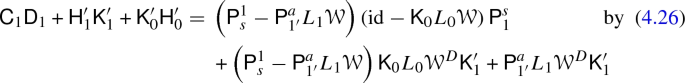
• 5. $\mathrm {id}_{1'} = \mathsf {C}_1 \mathsf {D}_1 + \mathsf {H}'_1 \mathsf {K}'_1 + \mathsf {K}'_0 \mathsf {H}'_0$:

  

  

  

• 6. $\mathrm {id}_1 = \mathsf {D}_1 \mathsf {C}_1 + \mathsf {H}_1 \mathsf {K}_1 + \mathsf {K}_0 \mathsf {H}_0$:

  

  

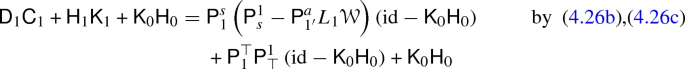
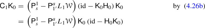
• 7. $\mathsf {K}'_1 \mathsf {C}_1 = \mathsf {C}_2 \mathsf {K}_1$                   by (4.26b),(4.26d)

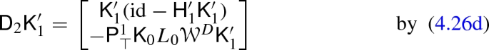
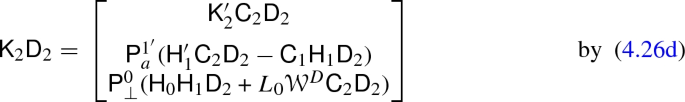
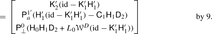
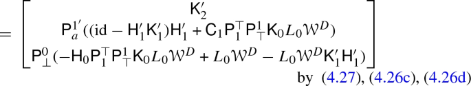
• 8. $\mathsf {K}_1 \mathsf {D}_1 = \mathsf {D}_2 \mathsf {K}'_1$:

  

  

  

• 9. $\mathrm {id}_{2'} = \mathsf {C}_2 \mathsf {D}_2 + \mathsf {H}'_2 \mathsf {K}'_2 + \mathsf {K}'_1 \mathsf {H}'_1$                   by (4.26d),(4.26e)

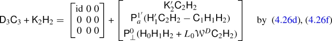
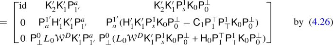
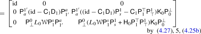
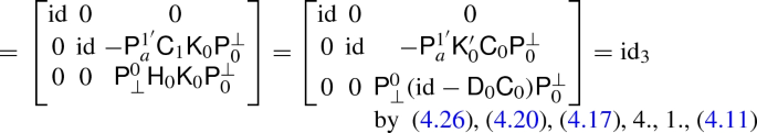
• 10. $\mathrm {id}_2 = \mathsf {D}_2 \mathsf {C}_2 + \mathsf {H}_2 \mathsf {K}_2 + \mathsf {K}_1 \mathsf {H}_1$:

  $$\begin{aligned} \mathsf {D}_2 \mathsf {C}_2 + \mathsf {K}_1 \mathsf {H}_1 + \mathsf {H}_2 \mathsf {K}_2 ={}&\begin{bmatrix} (\mathrm {id}- \mathsf {K}'_1 \mathsf {H}'_1) \mathsf {C}_2 \\ - \mathsf {P}^1_\top \mathsf {K}_0 L_0 {\mathcal {W}}^{D} \mathsf {C}_2 \end{bmatrix} + \begin{bmatrix} \mathsf {K}'_1 \mathsf {C}_1 \mathsf {H}_1 \\ \mathsf {P}^1_\top (\mathrm {id}- \mathsf {K}_0 \mathsf {H}_0) \mathsf {H}_1 \end{bmatrix}\\&+ \begin{bmatrix} \mathsf {K}'_1 \mathsf {P}^a_{1'} \mathsf {P}^{1'}_a (\mathsf {H}'_1 \mathsf {C}_2 - \mathsf {C}_1 \mathsf {H}_1) + \mathsf {K}'_1 \mathsf {P}^1_s \mathsf {K}_0 \mathsf {P}^\perp _0 \mathsf {P}^0_\perp (\mathsf {H}_0 \mathsf {H}_1 + L_0 {\mathcal {W}}^D \mathsf {C}_2) \\ \mathsf {P}^1_\top \mathsf {K}_0 \mathsf {P}^\perp _0 \mathsf {P}^0_\perp (\mathsf {H}_0 \mathsf {H}_1 + L_0 {\mathcal {W}}^D \mathsf {C}_2) \end{bmatrix} \\ ={}&\begin{bmatrix} \mathsf {K}'_1 (\mathsf {P}^a_{1'} \mathsf {P}^{1'}_a - \mathrm {id}) (\mathsf {H}'_1 \mathsf {C}_2 - \mathsf {C}_1 \mathsf {H}_1) + \mathsf {K}'_1 \mathsf {P}^1_s \mathsf {K}_0 \mathsf {P}^\perp _0 \mathsf {P}^0_\perp (\mathsf {H}_0 \mathsf {H}_1 + L_0 {\mathcal {W}}^D \mathsf {C}_2) + \mathsf {C}_2\\ \mathsf {P}^1_\top \mathsf {K}_0 (\mathsf {P}^\perp _0 \mathsf {P}^0_\perp - \mathrm {id}) (\mathsf {H}_0 \mathsf {H}_1 + L_0 {\mathcal {W}}^D \mathsf {C}_2) + \mathsf {P}^1_\top \mathsf {H}_1 \end{bmatrix} \\ ={}&\begin{bmatrix} \mathsf {K}'_1 \mathsf {P}^1_s ( \mathsf {K}_0 L_0 {\mathcal {W}}^D \mathsf {C}_2 + \mathsf {H}_1 - \mathsf {K}_0 \mathsf {H}_0 \mathsf {H}_1 ) + \mathsf {K}'_1 \mathsf {P}^1_s \mathsf {K}_0 (\mathsf {H}_0 \mathsf {H}_1 + L_0 {\mathcal {W}}^D \mathsf {C}_2) + \mathsf {C}_2\\ \mathsf {P}^1_\top \mathsf {H}_1 \end{bmatrix} \\ ={}&\begin{bmatrix} - \mathsf {K}'_1 \mathsf {P}^1_s \mathsf {H}_1 + \mathsf {C}_2\\ \mathsf {P}^1_\top \mathsf {H}_1 \end{bmatrix} = \mathrm {id}_2 \end{aligned}$$

  Here we used (13), (4.11), (4.25e), (4.20).

• 11. $\mathsf {K}_2 \mathsf {D}_2 = \mathsf {D}_3 \mathsf {K}'_2$:

  

  

  

  

  

  

  

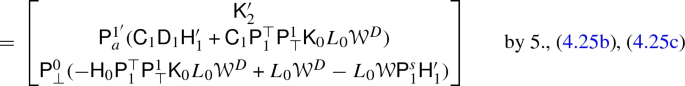
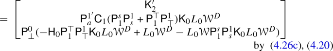
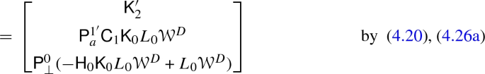
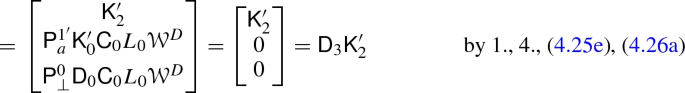
• 12. $\mathsf {K}'_2 \mathsf {C}_2 = \mathsf {C}_3 \mathsf {K}_2$                   by (4.26d), (4.26f)

• 13. $\mathrm {id}_{3'} = \mathsf {C}_3 \mathsf {D}_3 + \mathsf {H}'_3 \mathsf {K}'_3 + \mathsf {K}'_2 \mathsf {H}'_2$                   by (4.26e), (4.26f)

• 14. $\mathrm {id}_3 = \mathsf {D}_3 \mathsf {C}_3 + \mathsf {H}_3 \mathsf {K}_3 + \mathsf {K}_2 \mathsf {H}_2$:

  

  

  

  

• 15. $\mathsf {K}_3 \mathsf {D}_3 = \mathsf {D}_4 \mathsf {K}'_3$                   by (4.26f), (4.26g)

• 16. $\mathsf {K}'_3 \mathsf {C}_3 = \mathsf {C}_4 \mathsf {K}_3$                   by (4.26f), (4.26g)

Compositions of $\mathsf {K}$ operators yield

$$\begin{aligned} \mathsf {K}_1 \mathsf {K}_0 ={}&\begin{bmatrix} \mathsf {K}'_1 \mathsf {C}_1 \mathsf {K}_0 \\ \mathsf {P}^1_\top (\mathrm {id}- \mathsf {K}_0 \mathsf {H}_0) \mathsf {K}_0 \end{bmatrix} = \begin{bmatrix} \mathsf {K}'_1 \mathsf {K}'_0 \mathsf {C}_0 \\ \mathsf {P}^1_\top \mathsf {K}_0 \mathsf {D}_0 \mathsf {C}_0 \end{bmatrix}= \begin{bmatrix} 0 \\ \mathsf {P}^1_\top \mathsf {P}^s_1 \mathsf {K}'_0 \mathsf {C}_0 \end{bmatrix} = 0, \\ \mathsf {K}_2 \mathsf {K}_1 ={}&\begin{bmatrix} \mathsf {K}'_2 \mathsf {C}_2 \mathsf {K}_1 \\ \mathsf {P}^{1'}_a (\mathsf {H}'_1 \mathsf {C}_2 \mathsf {K}_1 - \mathsf {C}_1 \mathsf {H}_1 \mathsf {K}_1)\\ \mathsf {P}^0_\perp (\mathsf {H}_0 \mathsf {H}_1 \mathsf {K}_1 + L_0 {\mathcal {W}}^{D} \mathsf {C}_2 \mathsf {K}_1) \end{bmatrix} \nonumber \\ ={}&\begin{bmatrix} \mathsf {K}'_2 \mathsf {K}'_1 \mathsf {C}_1 \\ \mathsf {P}^{1'}_a (\mathsf {H}'_1 \mathsf {K}'_1 \mathsf {C}_1 - \mathsf {C}_1 \mathsf {H}_1 \mathsf {K}_1)\\ \mathsf {P}^0_\perp (\mathsf {H}_0 \mathsf {H}_1 \mathsf {K}_1 + L_0 {\mathcal {W}}^{D} \mathsf {K}'_1 \mathsf {C}_1) \end{bmatrix} \nonumber \\ ={}&\begin{bmatrix} 0 \\ \mathsf {P}^{1'}_a \mathsf {C}_1( \mathrm {id}- \mathsf {D}_1 \mathsf {C}_1 - \mathsf {H}_1 \mathsf {K}_1)\\ \mathsf {P}^0_\perp \mathsf {H}_0 (\mathsf {H}_1 \mathsf {K}_1 + \mathsf {D}_1 \mathsf {C}_1) \end{bmatrix} \nonumber \\ ={}&\begin{bmatrix} 0 \\ \mathsf {P}^{1'}_a \mathsf {C}_1 \mathsf {K}_0 \mathsf {H}_0\\ -\mathsf {P}^0_\perp \mathsf {H}_0 (\mathsf {K}_0 \mathsf {H}_0 - \mathrm {id}) \end{bmatrix} = \begin{bmatrix} 0 \\ \mathsf {P}^{1'}_a \mathsf {K}'_0 \mathsf {C}_0 \mathsf {H}_0\\ \mathsf {P}^0_\perp \mathsf {D}_0 \mathsf {C}_0 \mathsf {H}_0 \end{bmatrix} = 0, \\ \mathsf {K}_3 \mathsf {K}_2 ={}&\mathsf {K}'_3 \mathsf {C}_3 \mathsf {K}_2 = \mathsf {K}'_3 \mathsf {K}'_2 \mathsf {C}_2 = 0. \end{aligned}$$

$\square$

5 Equivalence of Invariants

Here we discuss the equivalence of $\mathsf {K}_1$ and the operators appearing in the set of invariants of [2] which we denote collectively by ${{\widetilde{\mathsf {K}}}}_1$. Recall that ${{\widetilde{\mathsf {K}}}}_1$ consists of the quantities⁴

$$\begin{aligned} \vartheta \Phi&: V_1 \rightarrow (2,2), \end{aligned}$$

(5.1a)

$$\begin{aligned} \vartheta \Lambda&: V_1 \rightarrow (0,0), \end{aligned}$$

(5.1b)

$$\begin{aligned} \mathcal {P}^{2} \vartheta \Psi&: V_1 \rightarrow (4,0), \end{aligned}$$

(5.1c)

$$\begin{aligned} {\mathbb {I}}_V&: V_1 \rightarrow (0,0), \qquad \text { for } V \in \{\xi ,\zeta \}. \end{aligned}$$

(5.1d)

The explicit forms of the operators are given in (3.18) and by

$$\begin{aligned} \mathcal {P}^{2} \vartheta \Psi \,{:=}{}\,&\begin{bmatrix} \tfrac{1}{2}\mathcal {P}^{2} \mathscr {C}\mathscr {C}&0 \end{bmatrix}, \end{aligned}$$

(5.2a)

$$\begin{aligned} {\mathbb {I}}_V \,{:=}{}\,&{\mathbb {I}}_V^{D}{\mathcal {W}}+ {\mathbb {I}}_V^{A}, \end{aligned}$$

(5.2b)

with $\mathcal {P}^2$ given in (3.12) and

$$\begin{aligned} {\mathbb {I}}_V^{A}&\,{:=}{}\,&\tfrac{81}{2} \Psi _{2} \kappa _{1}{}^3\begin{bmatrix} ( V \overset{1,1}{\odot } \xi \overset{1,1}{\odot } \mathcal {K}^0 \mathcal {K}^2\bullet - V \overset{1,1}{\odot } \xi \overset{1,1}{\odot } \bullet )&\tfrac{1}{4} V \overset{1,1}{\odot } \xi \overset{0,0}{\odot } \bullet \end{bmatrix}, \end{aligned}$$

(5.3a)

$$\begin{aligned} {\mathbb {I}}_V^{D}&\,{:=}{}\,&\begin{bmatrix} {\mathbb {I}}_V^{D1}&{\mathbb {I}}_V^{D2} \end{bmatrix}, \end{aligned}$$

(5.3b)

$$\begin{aligned} {\mathbb {I}}_V^{D1}&\,{:=}{}\,&-81V {\overset{1,1}{\odot }}\mathcal {K}^1\mathscr {T}( \kappa _{1}{}^4\mathcal {K}^2\mathcal {K}^2\bullet ) - \tfrac{81}{2}\kappa _{1}{}^4(\mathcal {K}^2\mathscr {C}V)_{}\mathcal {K}^2\mathcal {K}^2\bullet - 27\kappa _{1}{}^3V {\overset{1,1}{\odot }}\xi {\overset{1,0}{\odot }}\mathcal {K}^1\mathcal {K}^2\bullet ,\nonumber \\ \end{aligned}$$

(5.3c)

$$\begin{aligned} {\mathbb {I}}_V^{D2}&\,{:=}{}\,&- \tfrac{81}{2}{\bar{\kappa }}_{1'}{}^4(\overline{\mathcal {K}}^2\mathscr {C}^\dagger V)_{}\overline{\mathcal {K}}^2\overline{\mathcal {K}}^2\bullet + 27{\bar{\kappa }}_{1'}{}^3V {\overset{1,1}{\odot }}\xi {\overset{0,1}{\odot }}\overline{\mathcal {K}}^1\overline{\mathcal {K}}^2\bullet . \end{aligned}$$

(5.3d)

Applied to a linearized metric, $\vartheta \Phi$ and $\vartheta \Lambda$ are the trace-free and trace parts of linearized Ricci, $\mathcal {P}^{2} \vartheta \Psi$ are the linearized extreme Weyl components (Teukolsky scalars), cf. (3.18). ${\mathbb {I}}_V$ are two third order complex scalar invariants.

Neither the number of components nor the differential order of the two sets of invariants coincide and we refer to Sect. 6 for more details. Next we show that ${\widetilde{\mathsf {K}}}_1$ and $\mathsf {K}_1$ can be factored through each other, thereby proving the completeness of ${\widetilde{\mathsf {K}}}_1$.

5.1 Factorization of ${\widetilde{\mathsf {K}}}_1$ through $\mathsf {K}_1$

In this subsection we show that ${\widetilde{\mathsf {K}}}_1= {\widetilde{\mathsf {D}}}_2 \circ \mathsf {K}_1$ for some operator ${\widetilde{\mathsf {D}}}_2$. Following [23, Lemma 4], assume we have ${\widetilde{\mathsf {K}}}_1 \circ \mathsf {D}_1 = \mathsf {F}\circ \mathsf {K}_1'$, for some operator $\mathsf {F}$, then

$$\begin{aligned} {\widetilde{\mathsf {K}}}_1 ={}&{\widetilde{\mathsf {K}}}_1 \circ (\mathsf {D}_1 \circ \mathsf {C}_1 + \mathsf {H}_1 \circ \mathsf {K}_1 + \mathsf {K}_0 \circ \mathsf {H}_0) \nonumber \\ ={}&\mathsf {F}\circ \mathsf {K}_1' \circ \mathsf {C}_1 + {\widetilde{\mathsf {K}}}_1 \circ \mathsf {H}_1 \circ \mathsf {K}_1 \nonumber \\ ={}&(\mathsf {F}\circ \mathsf {C}_2 + {\widetilde{\mathsf {K}}}_1 \circ \mathsf {H}_1) \circ \mathsf {K}_1 \end{aligned}$$

(5.4)

Hence, we can choose ${\widetilde{\mathsf {D}}}_2 = \mathsf {F}\circ \mathsf {C}_2 + {\widetilde{\mathsf {K}}}_1 \circ \mathsf {H}_1$. Now we compute $\mathsf {F}$.

Definition 15

$$\begin{aligned} \vartheta \Phi ^{D} {:=}{}&\begin{bmatrix} k^1&\overline{k^1}&k^2&\overline{k^2} \end{bmatrix}, \text { with } \nonumber \\ k^i {:=}{}&\tfrac{1}{6}e^{i}{}{\overset{0,0}{\odot }}\mathscr {C}\bullet - \tfrac{1}{4}e^{i}{}{\overset{0,1}{\odot }}\mathscr {T}\bullet - \tfrac{1}{8}e^{1}{}{\overset{0,1}{\odot }}\Upsilon ^{i}{}_{1}{}{\overset{0,0}{\odot }}\bullet - \tfrac{1}{8}e^{2}{}{\overset{0,1}{\odot }}\Upsilon ^{i}{}_{2}{}{\overset{0,0}{\odot }}\bullet + \tfrac{1}{12}e^{1}{}{\overset{0,0}{\odot }}\Upsilon ^{i}{}_{1}{}{\overset{0,1}{\odot }}\bullet \nonumber \\&\quad + \tfrac{1}{12}e^{2}{}{\overset{0,0}{\odot }}\Upsilon ^{i}{}_{2}{}{\overset{0,1}{\odot }} \bullet , \end{aligned}$$

(5.5a)

$$\begin{aligned} \vartheta \Lambda ^{D} {:=}{}&\begin{bmatrix} r^1&\overline{r^1}&r^2&\overline{r^2} \end{bmatrix}, \text { with }\nonumber \\ r^i {:=}{}&- \tfrac{1}{24}e^{i}{}{\overset{1,1}{\odot }}\mathscr {C}\bullet - \tfrac{1}{48}e^{1}{}{\overset{1,1}{\odot }}\Upsilon ^{i}{}_{1}{}{\overset{0,1}{\odot }}\bullet - \tfrac{1}{48}e^{2}{}{\overset{1,1}{\odot }}\Upsilon ^{i}{}_{2}{}{\overset{0,1}{\odot }}\bullet . \end{aligned}$$

(5.5b)

Lemma 16

The operator ${\widetilde{\mathsf {K}}}_1$ composed with $\mathsf {D}_1$ factors through $\mathsf {K}_1'$ via ${\widetilde{\mathsf {K}}}_1\circ \mathsf {D}_1=\mathsf {F}\circ \mathsf {K}_1'$, where

$$\begin{aligned} \mathsf {F}={}&\begin{bmatrix} \vartheta \Phi ^{D}\\ \vartheta \Lambda ^{D}\\ \mathcal {P}^{2} \vartheta \Psi ^{D}\\ {\mathbb {I}}_\xi ^{D} {\mathcal {W}}^{D}\\ {\mathbb {I}}_\zeta ^{D} {\mathcal {W}}^{D} \end{bmatrix} \end{aligned}$$

(5.6)

Proof

The relations $\vartheta \Phi \mathsf {D}_1 = \vartheta \Phi ^{D} \mathsf {K}_1'$ and $\vartheta \Lambda \mathsf {D}_1 = \vartheta \Lambda ^{D} \mathsf {K}_1'$ are commutators of the linearized trace-free Ricci operator and linearized Ricci scalar operator (3.18) with the algebraic operator $\mathsf {D}_1$. For the Weyl components $\vartheta \Psi$ we use $\mathcal {P}^{2} \vartheta \Psi ^A = 0$ so that the factorization $\mathcal {P}^{2} \vartheta \Psi \mathsf {D}_1 = \mathcal {P}^{2} \vartheta \Psi ^{D} \mathsf {K}_1'$ follows from (4.25b). For ${\mathbb {I}}_V$ we find

$$\begin{aligned} {\mathbb {I}}_V^{A} \mathsf {D}_1 ={}&{\mathbb {I}}_V^{D} {\mathcal {W}}^{A} = 0, \qquad \text { for } V \in \{\xi ,\zeta \}, \end{aligned}$$

(5.7)

so that (5.2b) with (4.25b) leads to ${\mathbb {I}}_V \mathsf {D}_1= {\mathbb {I}}_V^{D} {\mathcal {W}}^{D} \mathsf {K}'_1$ for $V \in \{\xi ,\zeta \}$. $\square$

5.2 Factorization of $\mathsf {K}_1$ through ${\widetilde{\mathsf {K}}}_1$

In this subsection we show that $\mathsf {K}_1 = {\widetilde{\mathsf {C}}}_2 \circ {\widetilde{\mathsf {K}}}_1$ for some operator ${\widetilde{C}}_2$. For the second component of $\mathsf {K}_1$ we find the relation

(5.8)

The expansion of the first component of $\mathsf {K}_1$ in terms of $\widetilde{\mathsf {K}}_1$ required a long computation and the result is displayed in appendix A.

6 Counting Invariants

The conclusion from Sect. 5 is that the components of both operators $\mathsf {K}_1$ (computed using the methods of [23]) and ${\tilde{\mathsf {K}}}_1$ in (5.1) each constitute a complete set of local first order gauge invariants for metric perturbations of Kerr. Yet the two operators look quite different: $\mathsf {K}_1$ is of 4th differential order⁵ and has 15 real components, while ${\tilde{\mathsf {K}}}_1$ is of 3rd differential order and has 18 real components. So neither the degree nor the number of components is a stable quantity for a complete set of invariants under the kind of equivalence considered in Sects. 2 and 5. A natural question to ask is the following: is there any stable way to assign either an order or a number of components to a complete set of invariants, perhaps under some condition of minimality?

Practically speaking, the higher order of $\mathsf {K}_1$ is what allows it to get away with fewer components than ${\tilde{\mathsf {K}}}_1$. Taking differential linear combinations of the high order components of $\mathsf {K}_1$ it is possible to cancel the highest order coefficients, leaving behind the extra lower order components that are present in ${\tilde{\mathsf {K}}}_1$ but not in $\mathsf {K}_1$. It is also easy to see how, even without changing the number of components, the order of either $\mathsf {K}_1$ or ${\tilde{\mathsf {K}}}_1$ could be artificially inflated by mixing a high order derivative of one component with another, in an invertible way. The ambiguity in the order and in the number of components lies in the subtle interplay between the leading and sub-leading order coefficients in the gauge invariants.

This issue is very well known in the literature on overdetermined PDEs, where a set of relevant homological invariants has been identified, so-called Spencer cohomologies of a differential operator [19, 33, 35]. These invariants are stable under the kind of equivalence considered in Sects. 2 and 5 , and the dimensions of certain Spencer cohomologies can be combined to give the order and the number of components of the differential operator, provided it is in so-called involutive and minimal form. Minimality is a simple condition on the principal symbol, while involutivity is a more sophisticated condition involving both the principal and sub-principal parts of the operator.

The classical principal symbol $\sigma _p(\mathsf {K})$ of an operator $\mathsf {K}$ (the coefficients of highest differential order, contracted with covectors $p\in T^*M$ instead of partial derivatives) is most useful when every component of $\mathsf {K}$ has the same order. For operators of mixed orders, it is more useful to work with the graded symbol [25, 33], which is essentially the same as the weighted symbol of [13]. Using the same notation, the graded symbol $\sigma _p(\mathsf {K})$ is a matrix of homogeneous polynomials in the covector $p\in T^*M$, possibly of different orders but obeying some simple bounds, and it satisfies the convenient identity

$$\begin{aligned} \sigma _p(\mathsf {L}\mathsf {K}) = \sigma _p(\mathsf {L}) \sigma _p(\mathsf {K}) , \end{aligned}$$

(6.1)

even if the right-hand side is zero. The operator $\mathsf {K}$ is minimal⁶ when the rows of its symbol $\sigma _p(\mathsf {K})$ are linearly independent with respect to p-independent coefficients. And $\mathsf {K}$ is involutive⁷ when any admissible matrix of homogeneous polynomials $\lambda _p$ satisfying $\lambda _p \sigma _p(\mathsf {K})=0$ can be extended to a differential operator $\mathsf {L}$ (that is, $\sigma _p(\mathsf {L}) = \lambda _p$) such that $\mathsf {L}\mathsf {K}= 0$.

Minimality is easy to check, as it follows from maximality of numerical rank when $\sigma _p(\mathsf {K})$ is evaluated on a generic value of p. On the other hand, in general, it is much easier to show that $\mathsf {K}$ is not involutive (meaning that its degree or number of components has no invariant meaning) than the opposite. As an illustration, let us consider the involutivity of the Killing operator $\mathsf {K}_0$ on Kerr. Due to the fact that $\vartheta \Psi _2$ is gauge invariant in the Minkowski case, we have

$$\begin{aligned} \sigma _p (\vartheta \Psi _2) \sigma _p (\mathsf {K}_0) = 0. \end{aligned}$$

(6.2)

However, it can be shown that, on Kerr, there is no second order operator $\mathsf {L}$ with symbol $\sigma _p(\vartheta \Psi _2)$ such that $\mathsf {L}\mathsf {K}_0 = 0$, and hence $\mathsf {K}_0$ fails to be involutive. It was rightly noted in [29, 30] that constructing a full compatibility operator for an involutive version of $\mathsf {K}_0$ is much easier. However, we point out that our $\mathsf {K}_0$ is tied to the fixed notion of gauge symmetry and gauge invariance in linearized gravity, hence we are not free to replace it with its involutive prolongation. Preliminary analysis also indicates that neither $\mathsf {K}_1$ nor ${\widetilde{\mathsf {K}}}_1$ is involutive. We do suspect that enlarging ${\tilde{\mathsf {K}}}_1$ by $\mathfrak {I}\hat{{\mathcal {A}}}_3$ and $\mathfrak {I}\hat{{\mathcal {A}}}_4$ defined in Appendix A is sufficient to achieve involutivity. However, a full analysis of involutivity goes beyond the scope of this paper.

7 Discussion

In this paper we have given for the first time a proof of completeness for a set of gauge invariants for first order metric perturbations of the Kerr spacetime, where we have interpreted gauge invariants as compatibility operators for the Killing operator $\mathsf {K}$ on this background. In Sect. 4, we have constructed an operator $\mathsf {K}_1$ following the methods of [23], which guarantee that the components of $\mathsf {K}_1$ are a complete set of gauge invariants, even if their explicit expressions turn out to be somewhat cumbersome. In Sect. 5, we have shown that the operators $\mathsf {K}_1$ and $\widetilde{\mathsf {K}}_1$ factor through each other, where the $\widetilde{\mathsf {K}}_1$ consist of the concise set of gauge invariants introduced in [2], thus confirming the completeness of the components of $\widetilde{\mathsf {K}}_1$ that was stated in [2]. With little extra effort, the construction of Sect. 4 also yielded a full compatibility complex $\mathsf {K}_l$ for $\mathsf {K}_0 = \mathsf {K}$, terminating after $l=0,1,2,3$.

There exists a non-linear analog of the problem of constructing a complete set of linear gauge-invariants on a given background spacetime $(M,g_{ab})$. Namely, a so-called IDEAL characterization [12, 14,15,16] of a given spacetime consists of a list of tensors $\{T_i[g]\}$ covariantly built from the metric, Riemann tensor and covariant derivatives such that the conditions $T_i[g]=0$ are sufficient to guarantee that $(M,g_{ab})$ is locally isometric to the given reference spacetime. As was pointed out in the recent works [10, 24], where IDEAL characterizations were given for cosmological FLRW and Schwarzschild-Tangherlini black hole spacetimes, one can use the tensors $\{T_i[g]\}$ to construct linear gauge invariants on the characterized spacetime. In particular, the identity ${\mathcal {L}}_v T_i[g] = \dot{T}^g_i[\mathsf {K}^g[v]]$ [36] guarantees that the linear operator $\dot{T}^g_i[h]$ is a gauge invariant whenever $T_i[g] = 0$ (or even more generally when $T_i[g]$ is a combination of Kronecker-deltas with constant coefficients). Conversely, any linear metric perturbation $h_{ab}$ that leaves the local isometry class must violate the IDEAL characterization equalities, $\{T_i[g+h+\cdots ]\} \ne 0$, which is equivalent to $\{\dot{T}^g_i[h]\} \ne 0$, unless some $T_i$ vanish to a high order on the space of all metrics along some directions approaching the reference metric g. Thus, the operators $\{\dot{T}^g_i\}$ have a good geometric interpretation and provide a good candidate for a complete set of linear gauge invariants on the reference spacetime geometry. Checking their equivalence with a systematically constructed complete set of linear gauge invariants can accomplish a double goal: provide the complete gauge invariants with a geometric interpretation, and show that the set $\{\dot{T}^g_i\}$ is indeed complete. Such an exercise has already been successfully carried out for a class of FLRW geometries [18]. It would be worth while to complete the comparison, already initiated in [2], of the $\widetilde{\mathsf {K}}_1$ operator with the linearized IDEAL characterization of the Kerr spacetime given by Ferrando and Sáez [15].

It is well-known that the construction of Hodge–de Rham Laplacians on a Riemannian manifold uses in an essential way the structure of the de Rham complex as a compatibility complex. Similarly, it was observed in [22] that the compatibility complex $\mathsf {K}_l$ on a maximally symmetric Lorentzian spacetime can be endowed with a Hodge-like structure, producing a sequence of wave-like (normally hyperbolic [6]) operators $\square _l$, obeying the commutativity relations $\mathsf {K}_l \square _l = \square _{l+1} \mathsf {K}_l$. The $\square _l$ operators have several applications: (a) Providing a “Hodge theory” for the cohomology of the compatibility complex $H^*(\mathsf {K}_l)$ [21]. (b) Providing a propagation equation $\square _1 \mathsf {K}_1[h]$ directly for the gauge invariants of perturbations h satisfying the linearized Einstein equations. (c) Providing a reconstruction of the metric perturbation h from its invariants $\psi = \mathsf {K}_1[h]$, formally $h = \square _0^{-1}\delta _1[\psi ] = \delta _1[\square _1^{-1} \psi ]$, where $\square _l = \delta _{l+1} \mathsf {K}_{l+1} + \mathsf {K}_l \delta _l$. Alternatively, the metric reconstruction problem could be locally reduced to an application of the Poincaré lemma to the $\mathsf {K}'_l$ complex. It would be interesting to identify such a “Hodge-like structure” also for our $\mathsf {K}_l$ compatibility complex on Kerr.

In Sect. 6, we have discussed the notion of involutivity and minimality for a differential operator. Although it appears that $\mathsf {K}_0, \mathsf {K}_1, \widetilde{\mathsf {K}}_1$ fail to be involutive, it would be interesting to find an involutive and minimal version of the full compatibility complex $\mathsf {K}_l$, for $l\ge 1$, for instance by completing $\widetilde{\mathsf {K}}_1$ to involutivity as suggested at the end of Sect. 6 and lifting the rest of the $\mathsf {K}_l$ operators in an involutive way. Working with an involutive compatibility complex can simplify the search for a “Hodge-like structure” mentioned above. In the absence of involution, the differential orders of the operators $\delta _l$ are not a priori bounded from the known orders of the $\mathsf {K}_l$ and the expected orders of the $\square _l$ operators.

Although the Schwarzschild spacetimes are part of the Kerr family, the fact that they have a larger number of independent Killing vectors means that some of the discussion from this paper and the earlier paper [2] do not apply to them, so they need to be handled as special cases. In fact, the analogous construction of the compatibility complex for Schwarzschild spacetimes was already carried out in [23, Sec.3.3]. Also, in analogy with [2] for Kerr, a number of convenient sets of linear gauge invariants for Schwarzschild were given in [34]. It would be interesting to check whether any of these sets is complete by comparing them to the complete set of gauge invariants obtained in [23, Sec.3.3].

Finally, another application of the methods used in this paper would be the construction of a complete set of linear gauge invariants, as well as a corresponding full compatibility complex, for the Kerr–Newman charged rotating black hole spacetime. In the Kerr–Newman case, the compatibility complex must start with a more complicated operator $\mathsf {K}_0$ that incorporates both the linearized diffeomorphisms and the electromagnetic gauge transformations.

Component form of \({\widetilde{\mathsf {C}}}_2\)

For the frame (4.3) define the connection

$$\begin{aligned} \gamma ^{i}{}_{jk}\,{:=}{}\,&e^{a}{}_{j} e_{b}{}^{i} \nabla _{a}e^{b}{}_{k}. \end{aligned}$$

(A.1)

Define the spinors $\hat{\mathcal {A}}\in {\mathcal {S}}_ {1,1}$, , $P\in {\mathcal {S}}_ {2,2}$ and $Q\in {\mathcal {S}}_ {3,1}$ via

(A.2a)

(A.2b)

(A.2c)

(A.2d)

Also define tensor versions of P, Q and $\kappa$ via

(A.3a)

(A.3b)

(A.3c)

where $\sigma _{a}{}^{AA'}$ is the soldering form. Due to equations (56) and (58b) in [1] we get the relations

(A.4a)

(A.4b)

The definition of $\hat{\mathcal {A}}$ only differs by a $\vartheta \Phi$ term compared to $\mathcal {A}$ in [1]. From an argument in that paper one finds that $\mathfrak {I}\hat{{\mathcal {A}}}$ is gauge invariant. The components of $\mathfrak {I}\hat{{\mathcal {A}}}$ can be expressed algebraically in terms of ${\mathbb {I}}_\xi$, ${\mathbb {I}}_\zeta$ and P via

$$\begin{aligned} \mathfrak {I}{\mathbb {I}}_\xi ={}&-81 \mathfrak {I}\hat{{\mathcal {A}}}_{1},\quad \mathfrak {I}{\mathbb {I}}_\zeta ={}-81 \mathfrak {I}\hat{{\mathcal {A}}}_{2}, \end{aligned}$$

(A.5a)

$$\begin{aligned} P_{11} - \bar{P}_{11}={}&\frac{i M \mathfrak {I}\hat{{\mathcal {A}}}_{4}}{3 \kappa _{1}{} {\bar{\kappa }}_{1'}{}^3} + \frac{i M \mathfrak {I}\hat{{\mathcal {A}}}_{3}}{3 \kappa _{1}{}^3 {\bar{\kappa }}_{1'}{}} - \tfrac{2}{81}i \partial _{1}\mathfrak {I}{\mathbb {I}}_\xi , \end{aligned}$$

(A.5b)

$$\begin{aligned} P_{12} - \bar{P}_{12}={}&- \frac{3i M \mathfrak {I}\hat{{\mathcal {A}}}_{4} (\kappa _{1}{}^3 + \kappa _{1}{} {\bar{\kappa }}_{1'}{}^2 - 2 {\bar{\kappa }}_{1'}{}^3)}{4 \kappa _{1}{}^2 {\bar{\kappa }}_{1'}{}^3} - \frac{3i M \mathfrak {I}\hat{{\mathcal {A}}}_{3} (-2 \kappa _{1}{}^3 + \kappa _{1}{}^2 {\bar{\kappa }}_{1'}{} + {\bar{\kappa }}_{1'}{}^3)}{4 \kappa _{1}{}^3 {\bar{\kappa }}_{1'}{}^2}\nonumber \\&- \tfrac{1}{81}i \partial _{1}\mathfrak {I}{\mathbb {I}}_\zeta - \tfrac{1}{81}i \partial _{2}\mathfrak {I}{\mathbb {I}}_\xi . \end{aligned}$$

(A.5c)

Hence, we can conclude that any component of $\mathfrak {I}\hat{{\mathcal {A}}}$, P or Q can be expressed in terms of ${\widetilde{\mathsf {K}}}_1$.

For symmetric 2-spinors $\phi , \psi$, set

$$\begin{aligned} \begin{bmatrix} {\bar{\phi }} \\ \phi \\ {\bar{\psi }} \\ \psi \end{bmatrix} = \mathsf {K}'_1 \mathsf {C}_1 \end{aligned}$$

(A.6)

and define the real 2-forms

$$\begin{aligned} G_{ab}\,{:=}{}\,&\sigma _{a}{}^{AA'} \sigma _{b}{}^{BB'} ({{\bar{\epsilon }}}_{A'B'} \phi _{AB} + \epsilon _{AB} {\bar{\phi }}_{A'B'}) \end{aligned}$$

(A.7a)

$$\begin{aligned} H_{ab}\,{:=}{}\,&\sigma _{a}{}^{AA'} \sigma _{b}{}^{BB'} ({{\bar{\epsilon }}}_{A'B'} \psi _{AB} + \epsilon _{AB} {\bar{\psi }}_{A'B'}). \end{aligned}$$

(A.7b)

A long computer algebra calculation reveals that this operator factors through $\widetilde{\mathsf {K}}_1$ with components (5.1) via

$$\begin{aligned} M G_{12}&={}&- 54 (P_{12} + \bar{P}_{12}) - \tfrac{2}{3} \partial _{1}\mathfrak {R}{\mathbb {I}}_\zeta - \tfrac{2}{3} \partial _{2}\mathfrak {R}{\mathbb {I}}_\xi +108i \gamma ^{3}{}_{12} \mathfrak {I}\hat{{\mathcal {A}}}_{3} - 108i \gamma ^{4}{}_{12} \mathfrak {I}\hat{{\mathcal {A}}}_{4} , \end{aligned}$$

(A.8a)

$$\begin{aligned} M G_{13}&={}&\tfrac{2}{9} Y_{1}{}^{a} ( \partial _{a}{\mathbb {I}}_\xi + 162 P_{1a} -2 \gamma ^{2}{}_{1a} {\mathbb {I}}_\zeta - 2 \gamma ^{1}{}_{1a} {\mathbb {I}}_\xi ), \end{aligned}$$

(A.8b)

$$\begin{aligned} M G_{23}&={}&+ \tfrac{2}{9} Y_{1}{}^{a} \bigl (162 P_{2a} + \partial _{a}{\mathbb {I}}_\zeta -2i \gamma ^{2}{}_{2a} \mathfrak {I}{\mathbb {I}}_\zeta - 2i \gamma ^{1}{}_{2a} \mathfrak {I}{\mathbb {I}}_\xi - 54 (Q_{12a} + \bar{Q}_{12a})\bigr )\nonumber \\&- \tfrac{4}{9} Y_{2}{}^{a}(\gamma ^{2}{}_{1a} \mathfrak {R}{\mathbb {I}}_\zeta + \gamma ^{1}{}_{1a} \mathfrak {R}{\mathbb {I}}_\xi ) - \tfrac{4}{9}i \mathfrak {I}{\mathbb {I}}_\xi (\gamma ^{3}{}_{2a} Y_{3}{}^{a} - \gamma ^{4}{}_{2a} Y_{4}{}^{a}), \end{aligned}$$

(A.8c)

$$\begin{aligned} M G_{34}&={}&- 36i Y_{4}{}^{a} \partial _{1}\mathfrak {I}\hat{{\mathcal {A}}}_{a} +108i (\gamma ^{3}{}_{34} - 3 \gamma ^{4}{}_{33}) \mathfrak {I}\hat{{\mathcal {A}}}_{3} - 108i (3 \gamma ^{3}{}_{44} - \gamma ^{4}{}_{34}) \mathfrak {I}\hat{{\mathcal {A}}}_{4}\nonumber \\&- 36 (Q_{341} + \bar{Q}_{341}), \end{aligned}$$

(A.8d)

$$\begin{aligned} M H_{12}&={}&- 27 (P_{22} + \bar{P}_{22}) - \tfrac{2}{3} \partial _{2}\mathfrak {R}{\mathbb {I}}_\zeta + 54i \gamma ^{3}{}_{22} \mathfrak {I}\hat{{\mathcal {A}}}_{3} - 54i \gamma ^{4}{}_{22} \mathfrak {I}\hat{{\mathcal {A}}}_{4}, \end{aligned}$$

(A.8e)

$$\begin{aligned} M H_{13}&={}&\tfrac{2}{9} Y_{2}{}^{a} \bigl (162 P_{1a}+ \partial _{a}{\mathbb {I}}_\xi -i (\gamma ^{1}{}_{1a} + \gamma ^{2}{}_{2a}) \mathfrak {I}{\mathbb {I}}_\xi - 27 Q_{1a1} \bigr ) -18 Q_{231}\nonumber \\&- 18 (Q_{123} + \bar{Q}_{123}) - \tfrac{2}{9} \bigl (2 \gamma ^{2}{}_{2a} {\mathbb {I}}_\zeta + 2 \gamma ^{1}{}_{2a} {\mathbb {I}}_\xi - i (\gamma ^{1}{}_{1a} + \gamma ^{2}{}_{2a}) \mathfrak {I}{\mathbb {I}}_\zeta \bigr ) Y_{1}{}^{a}, \end{aligned}$$

(A.8f)

$$\begin{aligned} M H_{23}&={}&- \tfrac{2}{9} Y_{2}{}^{a} \bigl ( - 162 P_{2a} - \partial _{a}{\mathbb {I}}_\zeta +\gamma ^{2}{}_{2a} (2 {\mathbb {I}}_\zeta - i \mathfrak {I}{\mathbb {I}}_\zeta ) + i \gamma ^{1}{}_{1a} \mathfrak {I}{\mathbb {I}}_\zeta \nonumber \\&+ \gamma ^{1}{}_{2a} (2 {\mathbb {I}}_\xi + i \mathfrak {I}{\mathbb {I}}_\xi ) + 27 Q_{1a2}\nonumber \\&+ 27 (Q_{12a} + \bar{Q}_{12a}) \bigr ) - \tfrac{4}{3}i \gamma ^{1}{}_{23} \mathfrak {I}{\mathbb {I}}_\zeta - 18 Q_{232} - \tfrac{2}{9}i \mathfrak {I}{\mathbb {I}}_\xi (\gamma ^{3}{}_{22} Y_{3}{}^{1} - \gamma ^{4}{}_{22} Y_{4}{}^{1}), \end{aligned}$$

(A.8g)

$$\begin{aligned} M H_{34}&={}&18 \bar{Y}_{2}{}^{a}\bar{P}_{a3} - 18 Y_{2}{}^{a}P_{a4} - \tfrac{2}{9}i Y_{4}{}^{1} \partial _{1}\mathfrak {I}{\mathbb {I}}_\zeta + \tfrac{2}{9}i Y_{4}{}^{1} \partial _{2}\mathfrak {I}{\mathbb {I}}_\xi \nonumber \\&+ 36i \mathfrak {I}\hat{{\mathcal {A}}}_{3} (\gamma ^{1}{}_{2a} \bar{Y}_{1}{}^{a} - \gamma ^{1}{}_{1a} \bar{Y}_{2}{}^{a} + \gamma ^{4}{}_{2a} \bar{Y}_{4}{}^{a})\nonumber \\&+ 36i \mathfrak {I}\hat{{\mathcal {A}}}_{4} (\gamma ^{1}{}_{2a} Y_{1}{}^{a} - \gamma ^{1}{}_{1a} Y_{2}{}^{a} + \gamma ^{3}{}_{2a} Y_{3}{}^{a}) \nonumber \\&-9 Q_{234} + 27 Q_{243} - 27 Q_{342} - 9 \bar{Q}_{234} - 9 \bar{Q}_{243} - 9 \bar{Q}_{342}\nonumber \\&- 81 Q_{144} \kappa _{1}{} {\bar{\kappa }}_{1'}{} + 81 \bar{Q}_{133} \kappa _{1}{} {\bar{\kappa }}_{1'}{}\nonumber \\&+ \frac{81}{8 \kappa _{1}{} {\bar{\kappa }}_{1'}{}}(\bar{Q}_{144}- Q_{133}) (\kappa _{1}{}^2 + {\bar{\kappa }}_{1'}{}^2)^2 + (-81 Q_{134} + \tfrac{567}{4} Q_{143} - 81 Q_{341} - 81 \bar{Q}_{134} \nonumber \\&+ \tfrac{81}{4} \bar{Q}_{143}- \tfrac{81}{4} \bar{Q}_{341} - \frac{9 Q_{233}}{2 \kappa _{1}{} {\bar{\kappa }}_{1'}{}} + \frac{9 \bar{Q}_{244}}{2 \kappa _{1}{} {\bar{\kappa }}_{1'}{}}) (\kappa _{1}{}^2 + {\bar{\kappa }}_{1'}{}^2). \end{aligned}$$

(A.8h)

Here $M = 27 \Psi _{2} \kappa _{1}{}^3$ is the mass parameter of the Kerr solution.

References

Aksteiner, S., Andersson, L., Bäckdahl, T.: New identities for linearized gravity on the Kerr spacetime. Phys. Rev. D 99, 044043 (2019). arXiv:1601.06084 [gr-qc]
Aksteiner, S., Bäckdahl, T.: All local gauge invariants for perturbations of the Kerr spacetime. Phys. Rev. Lett. 121, 051104 (2018). arXiv:1803.05341
Andersson, L., Bäckdahl, T., Blue, P.: Second order symmetry operators. Class. Quantum Gravity 31, 135015 (2014). arXiv:1402.6252 [gr-qc]
Andersson, L., Bäckdahl, T., Blue, P., Ma, S.: Stability for linearized gravity on the Kerr spacetime (2019). arXiv:1903.03859 [math.AP]
Bäckdahl, T.: A formalism for the calculus of variations with spinors. J. Math. Phys. 57, 022502 (2016). arXiv:1505.03770 [gr-qc]
Baer, C., Ginoux, N., Pfaeffle, F.: Wave Equations on Lorentzian Manifolds and Quantization. ESI lectures in mathematics and physics, Vol. 2. European Mathematical Society (2007). arXiv:0806.1036
Barack, L., Ori, A.: Gravitational selfforce and gauge transformations. Phys. Rev. D64, 124003 (2001). arXiv:gr-qc/0107056 [gr-qc]
Blinkov, Y.A., Cid, C.F., Gerdt, V.P., Plesken, W., Robertz, D.: The MAPLE package Janet: I. polynomial systems. II. Linear partial differential equations. In: Ganzha, V.G., Mayr, E.W., Vorozhtsov, E.V. (eds.) Proceedings of the 6th International Workshop on Computer Algebra in Scientific Computing, Passau (Germany), pp. 31–54. Institut für Informatik, Technische Universität München, Garching (2003)
Calderbank, D.M.J., Diemer, T.: Differential invariants and curved Bernstein–Gelfand–Gelfand sequences. J. Reine Angew. Math. 537, 67–103 (2001)
Canepa, G., Dappiaggi, C., Khavkine, I.: IDEAL characterization of isometry classes of FLRW and inflationary spacetimes. Class. Quantum Gravity 35, 035013 (2018). arXiv:1704.05542
Čap, A., Slovák, J., Souček, V.: Bernstein–Gelfand–Gelfand sequences. Ann. Math. 154, 97–113 (2001)
Coll, B., Ferrando, J.J.: Thermodynamic perfect fluid Its Rainich theory. J. Math. Phys. 30, 2918–2922 (1989)
Douglis, A., Nirenberg, L.: Interior estimates for elliptic systems of partial differential equations. Commun. Pure Appl. Math. 8, 503–538 (1955)
Ferrando, J.J., Sáez, J.A.: An intrinsic characterization of the Schwarzschild metric. Class. Quantum Gravity 15, 1323–1330 (1998)
Ferrando, J.J., Sáez, J.A.: An intrinsic characterization of the Kerr metric. Class. Quantum Gravity 26, 075013 (2009). arXiv:0812.3310
Ferrando, J.J., Sáez, J.A.: An intrinsic characterization of spherically symmetric spacetimes. Class. Quantum Gravity 27, 205024 (2010). arXiv:1005.1780
Fröb, M.B., Hack, T.-P., Higuchi, A.: Compactly supported linearised observables in single-field inflation. J. Cosmol. Astropart. Phys. 2017, 043 (2017). arXiv:1703.01158
Fröb, M.B., Hack, T.-P., Khavkine, I.: Approaches to linear local gauge-invariant observables in inflationary cosmologies. Class. Quantum Gravity 35, 115002 (2018). arXiv:1801.02632
Goldschmidt, H.: Existence theorems for analytic linear partial differential equations. Ann. Math. 86, 246–270 (1967)
Jezierski, J.: Energy an angular momentum of the weak gravitational waves on the Schwarzschild backround-quasilocal gauge-invariant formulation. General Relat. Gravitat. 31, 1855 (1999). arXiv:gr-qc/9801068
Khavkine, I.: Cohomology with causally restricted supports. Ann. Henri Poincaré 17, 3577–3603 (2016). arXiv:1404.1932
Khavkine, I.: The Calabi complex and Killing sheaf cohomology. J. Geom. Phys. 113, 131–169 (2017). arXiv:1409.7212
Khavkine, I.: Compatibility complexes of overdetermined PDEs of finite type, with applications to the Killing equation. Class. Quantum Gravity 36, 185012 (2019). arXiv:1805.03751
Khavkine, I.: IDEAL characterization of higher dimensional spherically symmetric black holes. Class. Quantum Gravity 36, 045001 (2019). arXiv:1807.09699
Kruglikov, B.S., Lychagin, V.V.: Geometry of differential equations. In: Krupka, D., Saunders, D. (eds.) Handbook of Global Analysis, pp. 725–771. Elsevier, Amsterdam (2008)
Martel, K., Poisson, E.: Gravitational perturbations of the Schwarzschild spacetime: a practical covariant and gauge-invariant formalism. Phys. Rev. D 71, 104003 (2005). arXiv:gr-qc/0502028
Merlin, C., Ori, A., Barack, L., Pound, A., van de Meent, M.: Completion of metric reconstruction for a particle orbiting a Kerr black hole. Phys. Rev. D 94, 104066 (2016). arXiv:1609.01227
Penrose, R., Rindler, W.: Spinors and Space-time I & II. Cambridge Monographs on Mathematical Physics. Cambridge University Press, Cambridge (1986)
Pommaret, J.-F.: Minkowski, Schwarzschild and Kerr metrics revisited. J. Mod. Phys. 9, 1970–2007 (2018). arXiv:1805.11958 [physics.gen-ph]
Pommaret, J.-F.: Generating compatibility conditions and general relativity. J. Mod. Phys. 10, 371–401 (2019). arXiv:1811.12186 [math.DG]
Pommaret, J.F.: “A mathematical comparison of the Schwarzschild and Kerr metrics (2020). arXiv:2010.07001
Pound, A., Merlin, C., Barack, L.: Gravitational self-force from radiation-gauge metric perturbations. Phys. Rev. D 89, 024009 (2014). arXiv:1310.1513 [gr-qc]
Seiler, W.M.: Involution: The Formal Theory of Differential Equations and its Applications in Computer Algebra, Algorithms and Computation in Mathematics, vol. 24. Springer (2010)
Shah, A.G., Whiting, B.F., Aksteiner, S., Andersson, L., Bäckdahl, T. : Gauge-invariant perturbations of Schwarzschild spacetime (2016), arXiv:1611.08291
Spencer, D.C.: Overdetermined systems of linear partial differential equations. Bull. Am. Math. Soc. 75, 179–240 (1969)
Stewart, J.M., Walker, M.: Perturbations of space-times in general relativity. Proc. R. Soc. Lond. A Math. Phys. Sci. 341, 49–74 (1974)
Tarkhanov, N.N.: Complexes of Differential Operators, Mathematics and Its Applications, vol. 340. Kluwer, Dordrecht (1995)
Thompson, J.E., Chen, H., Whiting, B.F.: Gauge invariant perturbations of the Schwarzschild spacetime. Class. Quantum Gravity 34, 174001 (2017). arXiv:1611.06214 [gr-qc]
Thompson, J.E., Wardell, B., Whiting, B.F.: Gravitational self-force regularization in the Regge–Wheeler and easy gauges. Phys. Rev. D 99, 124046 (2019). arXiv:1811.04432 [gr-qc]
Walker, M., Penrose, R.: On quadratic first integrals of the geodesic equations for type \(\{2,2\}\) spacetimes. Commun. Math. Phys. 18, 265–274 (1970)
Acknowledgements
This work was completed while the authors were in residence at Institut Mittag-Leffler in Djursholm, Sweden during the fall of 2019, supported by the Swedish Research Council under grant no. 2016-06596. IK was partially supported by the Praemium Academiae of M. Markl, GAČR project 18-07776S and RVO: 67985840. The work of BFW was supported in part by NSF Grants PHY 1314529 and PHY 1607323 to the University of Florida. Support from the Institut d’Astrphysique de Paris (IAP), where part of this work was carried out, is also acknowledged, as is support at Astroparticule et Cosmologie (APC) from the French state funds managed by the ANR within the Investissements d’Avenir programme under Grants ANR-11-IDEX-0004-02 and ANR-14-CE03-0014-01-E-GRAAL. The authors are grateful to Prof. J.-F. Pommaret for several helpful discussions.
Funding
Open Access funding enabled and organized by Projekt DEAL. Open Access funding enabled and organized by Projekt DEAL.
Author information
Authors and Affiliations
Corresponding author
Additional information
Communicated by P.Chrusciel.
Publisher's Note
Springer Nature remains neutral with regard to jurisdictional claims in published maps and institutional affiliations.