

Abstract
The initial stages of transient luminous events (TLEs) occurring in the upper atmosphere of the Earth are, in a certain pressure range, controlled by the streamer mechanism. This paper presents the results of the first laboratory experiments to study the TLE streamer phenomena under conditions close to those of the upper atmosphere. Spectrally and highly spatiotemporally resolved emissions originating from radiative states  (second positive system) and
  (first negative system) have been recorded from the positive streamer discharge. Periodic ionizing events were generated in a barrier discharge arrangement at a pressure of 4 torr of synthetic air, i.e. simulating the pressure conditions at altitudes of ≃37 km. Employing Abel inversion on the radially scanned streamer emission and a 2D fitting procedure, access was obtained to the local spectral signatures within the over 106 m s−1 fast propagating streamers. The reduced electric field strength distribution within the streamer head was determined from the ratio of the
  band intensities with peak values up to 500 Td and overall duration of about 10 ns. The 2D profiles of the streamer head electric fields were used as an experimentally obtained input for kinetic simulations of the streamer-induced air plasma chemistry. The radial and temporal computed distribution of the ground vibrational levels of the radiative states involved in the radiative transitions analyzed (337.1 nm and 391.5 nm), atomic oxygen, nitrogen, nitric oxide and ozone concentrations are vizualized and discussed in comparison with available models of the streamer phase of Blue Jet discharges in the stratosphere.
Export citation and abstract BibTeX RIS
1. Introduction
Transient luminous events (TLEs) such as Sprites and Blue Jets in the upper atmosphere start with fast propagating ionization events called streamers [1–10]. These ionizing waves with a high self-generated electric field affect the local chemical environment in the upper atmosphere [11–16]. The knowledge of the streamer's electric field is crucial for understanding the initial conditions leading to the induced atmospheric chemistry. More precisely, the detailed spatiotemporal evolution of the electric field of the running streamer head is of particular interest as that is the primary location of the high-energy electrons contributing to the chemical changes. Streamers propagate with velocities reaching up to several percent of the speed of light, and their occurrence above the thunderclouds in the upper atmosphere is highly stochastic, which makes any field measurement difficult. Moreover, due to the relatively slow quenching of their optical emission in low-pressure air, it is not an easy task to obtain their instantaneous local parameters via spectrally resolved recordings without sufficient temporal resolution [17–21].
The access to spectrally resolved optical emissions of low-pressure streamers is of interest to derive possible nonequilibrium vibrational distribution functions of emitting molecular species and rotational temperatures [2, 17, 22]. Moreover, the mechanism underlying air heating by Blue Jets (BJ) and Giant Jets (GJs) is mainly driven by upward leaders preceded by a streamer corona that promotes the propagation of the leader [23]. As discussed in [23–25], fast heating is a key mechanism accounting for the energy released to neutrals through chemical reactions that is an indication of the streamer to leader transition. The experimental determinantion of the spatio-temporal evolution of the reduced electric field within streamers produced in electric discharges at 4 torr (approx. 37 km altitude) will allow us to determine the influence of streamers ahead of BJ leaders in the formation of species such as O(1D), N(2D) and N2(B ,
,  ) that, when quenched, are the main source of air heating at ground pressure and, less efficiently, at altitudes where BJ and GJ occur [23].
The electron density and mean energy or values of the electric field can be assessed for further study of the induced atmospheric chemistry or the overall electrical characteristics of the phenomena [3, 26, 27]. There are several observational results reporting estimation of electric field or the mean electron energy based on spectroscopic, time averaged, optical observations. Kuo et al [26] reported values of ≃400–655 Td for the reduced electric fields in the streamer region of GJs measured from the variation of the time-averaged spectral recordings of the intensity ratio of (0, 0) vibrational transitions of the first negative and second positive systems of molecular nitrogen. Morrill et al and Kanmae et al made similar determinations for streamers in Sprites [3, 27]. An ideal, yet still unavailable, situation improving the understanding would be to compare the determined parameters (electric field, selected species densities etc) from field observations with computer simulations—with all these parameters determined with sufficient spatial and temporal resolution covering the fundamental mechanisms of the ultra-fast phenomena. In fact, to determine any streamer's basic plasma parameters with appropriate spatiotemporal resolution is a challenging task even in well-equipped spectroscopic laboratories [17, 18].
In order to better understand real TLEs, we approached this task experimentally by reproducing in the laboratory similar conditions to those found in the upper atmosphere. Choosing the ideal laboratory discharge to simulate the TLE streamers (at least to a certain extent, see the limitations/corrections in [21, 28, 29]) is not an easy task. One possibility is to apply high voltage pulses to metallic needle electrodes to produce stochastically branching streamers in centimetre gaps. Intensified CCD recordings then deliver the macroscopic parameters and effects such as the streamer diameter, branching length, streamer reconnection, and mean velocity [28, 30, 31]. However, to be able to resolve a fine spectral structure with high spatiotemporal resolution a well stabilized, reproducible non-branching streamer discharge is necessary allowing the accumulation of the weak and extremely fast signals. Accumulative PMT recordings, streak or photon-counting techniques have to be applied [18, 32].
In this paper we present our results on the highly-resolved spatiotemporal determination of the electric field in streamer heads produced in a laboratory barrier discharge arrangement. Subsequently, we apply these electric field values as an input for the study of the streamer induced chemistry in low-pressure air plasmas. The present paper is divided into the following sections. In the next, second section, the experimental setup and equipment is described. In the third section the overall electrical and spectral characterisation of the discharge under investigation is described together with the mathematical methods used for the signal processing. The fourth section describes the method used for determining the electric field, as well as the approach followed for extrapolating the data to lower electric fields. Also the derived distribution of the 2D electric field is presented and discussed. In the fifth section, the streamer-induced plasma chemistry is described, analysed, and compared with the available results about Blue Jet discharges taking place in the range of pressure and altitude investigated in the present paper.
2. Experimental setup
The discharge arrangement was as follows. Two Macor® glass-ceramic discs with embedded metallic (point/plate) electrodes at a distance of 4 cm from each other were placed in a vacuum steel chamber with quartz glass windows. This dielectric barrier discharge setup allowed a better stabilization of the streamer occurrence temporally as well as spatially. Before every experiment, the chamber was evacuated to 0.5 torr and then flushed by synthetic air at a pressure of 4 torr for 20 min. The discharge was fed with synthetic air through a Bronkhorst HI-TEC mass-flow controller (with a fixed flow of F = 25 sccm). The pressure in the chamber was regulated by using a needle valve backed by an oil-free diaphragm vacuum pump (KNF Laboport), and measured by a TPG 260 piezo gauge (Pfeifer Vacuum).
In order to be able to trigger the streamer discharge ignition with high precision, a complex voltage waveform was applied [33]. The discharge was powered by an HV power supply superimposing AC waveforms with a positive pulse. The AC HV was produced by a TG1010A DDS function generator (TTi), Powertron Model 250A RF amplifier and an HV step-up transformer. The waveforms ( kHz) were amplitude modulated to give bursts of two consecutive sine-wave cycles fired at a fixed repetition frequency of
  Hz and voltage amplitude 1.5 kV producing HV AC ON/OFF periods (with duration
  ms and
  ms, see figure 1). A home-made pulse power supply was used to generate the positive HV pulse of 2 kV amplitude (FWHM ∼150 ns long, typical rising slope of 200 V ns−1, repetition rate
  =
=  ) by discharging a 10 nF capacitor through a Behlke Model HTS-81 solid state switch (8 kV DC/30 A, typical turn-on rise time 9 ns). Superposition of the two (AC and pulsed) HV waveforms with a suitable phase shift was done by means of a passive LC filter. A BNC Model 575 digital delay/pulse generator was used as the master trigger for the TG1010A function generator to synchronise the AC waveforms with the HV pulse. The stability of the current and voltage waveforms was controlled using a current probe Pearson 2877 and high-voltage probe Tektronix P6015A, respectively. The discharge was run under selected conditions for at least 10 min prior each measurement.
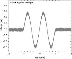
Figure 1. Voltage waveform applied to the inter-electrode gap with 4 torr pressure synthetic air with repetition of 30 Hz. The burst consists of a sequence of two sinusoidal waveforms (1.5 kV amplitude) superposed with a 2 kV high-voltage nanosecond pulse (at the time t = 0 ms) to trigger the discharge at the right moment.
Download figure:
Standard image High-resolution imageOptical emission was recorded by PMT (Hamamatsu H10721, rise-time of 200 ps) via 25 cm long capillary with an inner diameter of 1 mm. In order to record only spectrally selected emission of the first negative and second positive system band, a set of suitable bandpass filters was utilized. For the signal of the second positive system (SPS) 0-0 vibrational transition, band head at 337.1 nm the bandpass filter with FWHM of 9.7 nm was used (LOT Oriel 337FS10). For the 391.5 nm wavelength, a Semrock FF01-395/11 filter (central wavelength 395 nm, FWHM 16.1 nm) was used, and for 370 nm, a Semrock FF01-370/10 filter (central wavelength 370 nm, FWHM 11.5 nm). The temporally resolved spectra (spectral kinetic series) were recorded on an ICCD camera (Andor DH740i-18U-03 iStar) via an iHR-320 (Jobin-Yvon) spectrometer. For this purpose a larger opening of 8 mm diameter was used in order to get a reasonable signal. This was performed at a distance of approximately 15 mm from the cathode.
3. Electrical analysis and spectrally resolved streamer emission
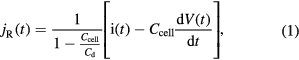
Triggered early stage streamers were generated within the barrier discharge with a repetition frequency of the burst, i.e. 30 Hz. Using electrical probes, the instantaneous current and voltage waveforms were recorded in the external electrical circuit of the discharge setup. Note that using electrical probe measurements in the external circuit of the barrier discharge, one does not get the exact electrical parameters of the plasma, due to the capacitive coupling of the dielectric barriers. Thus, the measured values have to be corrected by a factor derived from the characteristic capacitances of the setup. We followed the theory given in [34] and determined the correction factor using the method of Pipa et al [35]. The equation describing the current in the plasma is (according to [34])
where  is the measured current,
  is the capacitive current (which can be measured for the same electrical conditions only at an elevated gas pressure, where the discharge does not happen, and subtracted) and
  and
and  are the characteristic capacitances of the barrier discharge setup. These capacitances were determined from the charge–voltage, i.e. Q–V plot, see figure 2(a). The capacitance
  is determined from the 'capacitive charge' increase prior to the breakdown. The capacitance
  is determined from a linear fit of the points of maximal charge values for different amplitudes of the applied voltage pulses as proposed in [35]. The equation for the correct electrical charge transfer within the plasma is obtained by integrating equation (1) over time. The corrected plasma parameters of the current and the charge are presented in figure 2(b). The electric current of a single triggered discharge reached a peak value of 1000 mA with a FWHM equal to 30 ns of the current profile. The charge transferred by a single discharge has a value of 35 nC. According to its temporal development and final saturation, the overall electrical discharge duration does not exceed 100 ns by very much. Using the results in [34] one can compute also the real gap voltage, i.e. the true voltage applied onto the gas in the gap without influence of the dielectric barriers (see in figure 3). Dividing this gap voltage by the real discharge current one can obtain the resistance of the plasma. The development of instantaneous electrical resistance is shown in figure 3. At the time of 0 ns the first charge transfer happens. At the 20th nanosecond the streamer impacts onto the cathode and the resistance is approximately 2000 V A−1. Ten nanoseconds later, a discharge filament is created and the resistance goes down to approx. 1000 V A−1.
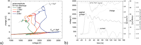
Figure 2. Q–V plot constructed for determination of characteristic capacitances of the 4 torr setup discharge (a) and corrected electrical parameters of the barrier discharge with SPS recording via PMT, temporally synchronized (b). The empty circles in part (a) denote truncated Q–V dependency for further irrelevant values.
Download figure:
Standard image High-resolution image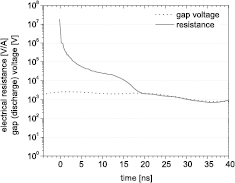
Figure 3. Dividing the real gap voltage and current waveform one can obtain the instantaneous electrical resistance of the discharge. In the 30th nanosecond (at the maximal SPS signal, see figure 2) the resistance value is approximately 1000 V A−1. For effective radius of 1 cm (see further in the text) and length of 4 cm the conductivity of the resulting transient plasma channel is approx. 0.13 S m−1.
Download figure:
Standard image High-resolution imageIn figure 2(b), the temporally correlated emission of the SPS (0, 0) vibrational transition band is shown recorded using the capillary, interference filter and photomultiplier. One can see that the emission starts simultaneously with the current rise, reaching its maximum 20 ns later. The SPS spectral bands contribute primarily to the barrier discharge emission. Accordingly, the temporally correlated spectral kinetic series are shown in figure 4. Besides the emissions of the SPS bands, the FNS (0, 0) vibrational transition band is visible as well. The SPS bands peak at 30 ns, the same time as in figure 2(b). Nevertheless, the FNS emission reaches its maximum approximately 10 ns earlier. At the 20th nanosecond of the emission development, the FNS signal marks the presence of a higher electric field with electrons reaching an energy of almost 19 eV. At this time the streamer crosses the gap.
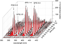
Figure 4. Kinetic series of the air discharge spectra around 400 nm for 4 torr pressure. This time-resolved spectra (time indicates a delay between the trigger and ICCD gate) were acquired via a larger opening of 8 mm diameter with centre positioned 15 mm axially from the cathode using a 5 ns ICCD gate width. The larger opening was necessary due to the weak signal. Clearly, one can see that the maximum of the FNS (0, 0) emission precedes the SPS bands' maxima in time (compare [18]).
Download figure:
Standard image High-resolution image4. Determination of radially and temporally resolved E/N
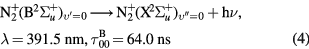
The electric field determination is based on the measured emissions of the spectral bands of the second positive (SPS (0, 0) vibrational transition band head at wavelength 337.1 nm, upper state of N2(C )) and first negative (FNS (0, 0) vibrational transition band head at wavelength 391.5 nm, upper state N
 (B
(B )) systems of molecular nitrogen [36], see the following equations. Equations (2) and (3) describe the direct electron impact excitation/ionization via high energy electrons, Equations (4) and (5) describe the radiative de-excitation with corresponding wavelengths and radiative constants, and equations (6) and (7) describe the collisional de-excitation by molecular nitrogen and oxygen with corresponding effective radiation times for 4 torr pressure air [37–39].


These SPS and FNS emissions were recorded via interference filters placed before the capillary and PMT entrance. The measured emissions for these spectral filters are shown in figures 6(a) and (c). The emission FNS waveform sampled in the region of the (0, 0) band must be corrected appropriately, because the FNS (0, 0) band always overlaps the tail of the SPS (2, 5) band [40]. In the case of the FNS (0, 0) waveforms obtained in this research, we used an alternative approach based on sampling part of the  sequence of the SPS in the 366–375 nm spectral range. After being multiplied by the appropriate constant, this waveform was used to subtract the SPS contribution from the mixed FNS (0, 0) and SPS (1, 4) + SPS (2, 5) + SPS (3, 6) waveforms. The appropriate constant was determined by simulating the SPS emission [17] at
  K using the experimentally determined vibrational distribution of the
  state. The synthetic SPS spectrum was multiplied by the transmittance of both (371/391 nm) filters, corrected for quantum efficiency of the H10721 photocathode, and finally integrated over the spectral regions covered by the two filters. The ratio of the two integrals then provides the required constant.
4.1. Two-dimensional data fitting
Despite the very careful experimental setup for recording the PMT signals, the radial scans of the temporal profiles of the optical emission (337 nm and 395 nm filter recordings) may suffer from a low noise-to-signal ratio as well as from strong spurious oscillations. These disruptive effects mean that using simple noise filters or data smoothing to process the individual temporal profiles gives inherently poor and unreliable results. Thus, we developed a fitting procedure that allows taking into account all radial scans at once. Following the approach for Abel inversion from [41], a Gaussian profile is assumed for the radial distribution of the optical emission signal of the discharge at any given time:
where I0(t) is the amplitude,  is the characteristic width of the signal at time t, and x is a radial coordinate. Because the PMT recording of the optical emissions features a sharp rise followed by a slower decay, we have adopted a double-sigmoid function for parametrization:
where {pj} are parameters to be determined by fitting. The double-sigmoid is advantageous since it asymptotically approaches the initial and the final state, thus avoiding physically unreasonable overshoots. The characteristic width of the signal is parametrized using a simple quadratic function

where {qi} are parameters. Let  be the temporal profiles of the optical emission at the radial positions
 ![$x\in \left[-12,\ldots,12\right]$](https://content.cld.iop.org/journals/0963-0252/25/4/045021/revision1/psstaa2cd5ieqn026.gif) consisting of Np = 1000 discrete data points at
consisting of Np = 1000 discrete data points at ![$t\in \left[1,\ldots,{{N}_{p}}\right]$](https://content.cld.iop.org/journals/0963-0252/25/4/045021/revision1/psstaa2cd5ieqn027.gif) . For the purpose of fitting, the set of
. For the purpose of fitting, the set of  is arranged into a 1D array
  with linear indexing ξ:

A function  is then fitted to
  at the discrete points ξ via the parameters {pj}, {qi} using model (9) with mapping


The Levenberg–Marquardt nonlinear regression algorithm from the optim toolbox of GNU Octave [42] is used for this purpose. Figure 5 shows the data sets  for the SPS and FNS optical emission PMT signals together with the fitted model (9) as a function of the linear index ξ. In spatiotemporal graphs in figure 6, the original measured 2D-data ((a) and (c)) and the fitted 2D-profiles (for FNS with subtracted overlap with neighbouring SPS (2,5)) and after Abel inversion are shown ((b) and (d)).
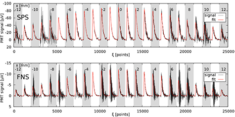
Figure 5. Radial scans of temporal profiles of SPS and FNS optical emission of the discharge. Temporal records for each radial position consist of 103 points and are arranged in a 1D array with mapping (11). Curves: PMT signals (black) and fit (red) using model (9).
Download figure:
Standard image High-resolution image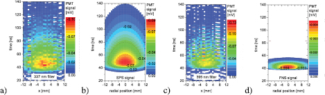
Figure 6. Radially and temporally resolved scans of the whole discharge emission (streamer emission just around the 40th nanosecond, see further) using 337 nm filter (a). In (b), the corresponding two-dimensionally fitted emission of the SPS band at 337 nm is determined for further processing. In (d), the deconvolved FNS signal is obtained from the 395 nm filter recordings (c) by subtracting the overlap with the neighbouring SPS (2,5) spectral band as described in the text. Compare figure 4. For more details about the subtraction, see the text. Time here indicates the delay elapsed from the oscilloscope's trigger. Note that these scans were recorded for different trigger settings and thus they are not temporally correlated with the recordings in the previous figures. The delay is approximately 20 ns.
Download figure:
Standard image High-resolution image4.2. The proper discharge part selection: propagating streamer, its velocity and diameter
The velocities of the streamers were estimated from the axial scans, see the example of the integral unfiltered emission signal from the 4 torr discharge in figure 7. Within the first 42 ns, two different phases of the signal development towards the cathode can be resolved: diffuse ionization wave initially with a low velocity (blue area), and subsequently with much higher velocities (no color). The axial development of the barrier discharge here is quantitatively identical to that known from atmospheric pressure discharges, whether sinusoidal or pulsed [32, 43, 44]: The discharge starts with a short charge accumulation phase during the first nanoseconds of the high-voltage pulse (see the electrical measurements in figure 2): the so-called pre-breakdown phase. It is followed by the phase of the ionization wave and cathode directed streamer propagation, its impact onto the cathode, and the creation of a transient glow discharge structure in the gap. Finally, the electric field in the gap decreases due to the charge deposition onto the dielectrics and the emission is quenched [32, 43, 44].
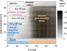
Figure 7. Axial scan of the discharge integral emission at 4 torr. The propagation of the streamer is denoted by dotted lines, which serve also for estimation of the actual streamer velocity, which is written beside them. The development of the discharge emission is typical for barrier discharges: an anode glow as well as a cathode layer is visible. The emission decays for over 100 ns. Note that this signal is correlated with the radial scans and electric field development in figures 6, 8, 9, 10 and with the results of kinetic model.
Download figure:
Standard image High-resolution imageThe PMT recordings presented here do not attain the sensitivity of the streak camera or the time-correlated single photon counting techniques, so the excitation processes in the short pre-breakdown phase are not visible in this by-pulse-initiated breakdown. However, the fast ionization wave moving from the anode towards the cathode is well visible. The velocity apparently increases from the initial  m s−1, through
  m s−1 (at the position of the PMT measurements in figure 6), and up to
  m s−1 close to the cathode for the 4 torr pressure streamer. Similarly to Yourgelenas and Wagner [44], the low velocity phase corresponds to the so-called diffuse part of the development of the barrier discharge ionization, while the high velocity phase corresponds to the streamer propagation. This point of view can be applied to the development of any higher-pressure filamentary barrier discharge, independently of whether pulsed or sine (compare [43]).
Furthermore, from the deconvolved radially resolved SPS data (see figure 6(b)), we have determined the radius of the streamer using following method. The radial emission profile of the SPS in the time of streamer passage (at 39th ns, see figures 7 and 8) was plotted and the FWHM dimension was determined. This gives the radius value of approximately 9 mm. It is important to note that it is not possible to built a completely scalable experimental setup, i.e. electrode spacing, and to have a streamer discharge stable enough to perform advanced spectroscopy studies at the same time (as mentioned already in the introduction). The radial emission profile gives the estimation of the streamer radius of 9 mm (compare [46] for similar pressure conditions). Clearly, the limited space between the electrodes of 4 cm is not allowing the streamer in our experiment to be fully developed. Nevertheless, we still observe high electric field enhancement (see further in the text) and a contracted discharge with a finite radius that is propagating at streamer-like velocities, therefore we believe that this allow us to say that we study a streamer at an early stage of development.
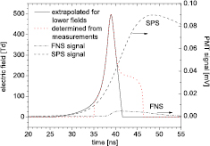
Figure 8. Electric field distribution in axial position in time (red dotted line) for a 4 torr streamer, determined from experimental measurements. The black solid line denotes the reconstructed electric field distribution in time using the Kulikovsky approach from [52] also for lower values of the electric field. The measured FNS and SPS signals, from which the field is determined, are shown as well. Note that these emission signals are for later times (approx. >42 ns) convolution of the streamer and the starting transient glow phase emission of the discharge, i.e. emitted not only by the streamer itself (for comparison see figure 7 and for pure streamer emission see results of the kinetic model in figure 12). This fact however does not disturb the determination of the electric field here. The sufficiently high time resolution of the PMT allows proper separation of the emission from subsequent discharge phases.
Download figure:
Standard image High-resolution imageTo summarize, we have run a stable barrier discharge in 4 torr pressure air. We have selected the emission part corresponding to the streamer only and used it for the electric field distribution determination (see next section). In subsequent step, only the streamer electric field has been used to show the long-duration chemistry induced solely by the streamer as it propagates free of other excitation/ionization mechanisms.
The first field observation of enhanced FNS emission in Blue Jets was reported by Wescott et al in [45] (first proposed in [6]). Later, Kuo et al [26] measured the spatially resolved emissions of the FNS and SPS systems for Blue Jet events. Also, from their photometers, Kuo et al estimated the speed of the propagation of the event to be on the order of 107 m s−1. Liu and Pasko made simulations of streamers under similar pressure conditions (30 km altitude, i.e. approximately 11 torr) in [46]. The velocity of the simulated streamer was  m s−1, which is directly comparable with the velocity of
  m s−1 obtained in the present paper.
4.3. Method of determining the electric field
The ratio of the intensities of the FNS and SPS is directly proportional to the reduced electric field strength [36]:

According to recent results [47, 48], this dependence (the right hand side of the equation (14)) should be divided by a factor of two and in such a form it is used further in the present paper. Nevertheless, the important comparison with the original form is also presented, see further in the text and in figure 9.
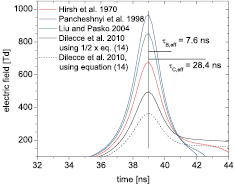
Figure 9. Influence of the chosen quenching constants and ratio multiplication factor on the determination of the development of the reduced electric field strength. The data are shown without the extrapolation procedure for low fields, as the result focuses on the peak magnitude. The effective lifetimes are shown for the quenching set of Dilecce et al [37].
Download figure:
Standard image High-resolution imageAs the streamer velocity remains at values on the order of 106 to 107 m s−1 over a wide pressure range [50], the sub-nanosecond time resolution of the spectroscopic device is crucial [18] even for lower pressures. It is absolutely necessary to resolve the rising edge of the streamer head emission for both spectral bands. For such a rapidly changing emission intensity, as it in the streamer head, the time-dependent form of the FNS to SPS ratio [18] has to be used. It results from the differential equations representing the dominant processes as given in equations (2)–(7) [51]:
where I denotes the intensity of the band emission and  the corresponding effective lifetime. The
  used were computed according to the definition in [39] based on experimentally obtained constants from [37–39].
The profile of the electric field in the centre of the discharge radial symmetry determined by the ratio method is shown in figure 8 by the red dotted line together with the recorded and fitted SPS and FNS signals. From the temporal development of both signals with respect to the electric field peak one can not directly observe mutual delays of signal maxima as observed and analysed for atmospheric pressure in [18]. The slow quenching and the subsequently created transient glow discharge structure (as described above) mutually interfere and thus these effects can not be attributed exclusively to the streamer-induced excitation/ionization.
The determined electric field values in figure 8 for times prior to 34 ns and after 42 ns suffer from a larger uncertainty, as the recorded FNS emission was too weak and/or noisy, and were disregarded in the further analysis. In order to reconstruct the electric field also in these low field regions, the profile was extrapolated according to the Kulikovsky model (black solid line in the graph) as proposed for a streamer head based on numerical simulations in [52] and experimentally confirmed also by Sretenovic et al [53]. In fact, the electrical field of the streamer head can be described by following the analytical expression [52]
where  is the peak value of the electric field produced by the space charge, lp is the width of the space charge layer, and x is the actual space coordinate at which the field is reconstructed. The x coordinate can be easily replaced by the time t via the known velocity. The electric field has its peak value at x = 0. Repeating the extrapolation process for noisy signal areas for all radial coordinates recorded, the radial and temporal distribution of the electric field can be obtained in a 2D graph, as shown later in figure 10.
Figure 10. 2D radially and temporally resolved electric field distribution in the streamer head in 4 torr determined from the experiments, panel (a). The peak value is 500 Td. The reduced electric field strength scale is logarithmic. The development of the radial structure of the electric field distribution in time is shown in (b).
Download figure:
Standard image High-resolution imageAn important parameter which can significantly influence the final result of the electric field determination is the chosen set of quenching constants. The influence of different quenching sets was presented in [37, 49] for constant electric fields. In figure 9, the development of the reduced electric field strength on a sub-nanosecond time scale is shown for several sets of quenching parameters, see table 1. In all cases, the same measured data for FNS and SPS intensities are used as an input for the computation. Note that the ratio of the effective lifetimes of selected nitrogen states  is very important, as equation (15) is directly proportional to its value. In figure 9, the corresponding effective lifetimes of the radiative states for 4 torr are shown as well, with respect to the electric field peak. While for the ICCD camera nanosecond recordings these several nanosecond long lifetime durations would result in incorrect values of the determined reduced electric field strength, for the here presented sub-nanosecond PMT resolution recording and the differential form of equation (15) used, that is not the case.
Table 1. Quenching rate constants (10−10 cm3 s−1) for evaluation of the effective lifetimes used in equation (15) for determining E/N.
 quenched by quenched by |
 quenched by quenched by |
|||
|---|---|---|---|---|
| N2 | O2 | N2 | O2 | |
| Dilecce [37], used here |  |
 |
 [39] [39] |
 [39] [39] |
| Hirsh [54] |  |
 |
 [39] [39] |
 [39] [39] |
| Pancheshnyi [55] |  |
 |
 [39] [39] |
 [39] [39] |
| Liu and Pasko [46] | 4 | 0 | 0 [46] | 3 [46] |
Note: As the quenching constants for  differ less from case to case, we further describe the complete set according to the constants for
  .
.
As mentioned above, we used here a novel form of the  dependence. The effect of the multiplication factor of 1/2 is shown in figure 9 as well. Multiplying equation (14) by 1/2, the electric field magnitude increases in its maximum by about 130 Td. This occurs with the
  quenching constants from Dilecce et al [37]. In this way, the determined electric field is used further for kinetic modelling of the induced plasma chemistry.
In order to confirm the magnitude of the obtained electric field profile we transformed the electric field profile in time (as shown in figure 8) to the space dimension over the actual velocity and integrated over the space. Comparing the resulting value of the electric potential difference to the obtained gap voltage from the electric measurements we are well within the error interval. Paris et al assessed the error of the method for determining E/N as approximately 10% (see [36] for more details). From our control measurements (repeating the experiment under the same conditions for the FNS signal), the electric field peak value varied within 20% of its value.
4.4. Radial and temporal electric field profile
In figure 10, the spatiotemporally resolved electric field distribution in the streamer head is shown for pressure of 4 torr. The electric field peaks at 500 Td and propagates with an instantaneous velocity of  m s−1 at the axial coordinate of 30 mm (see figure 7). The streamer head field distribution is restricted to a given radial area. The values of the electric field on the outer edges of these areas are conditioned by low FNS signal values, and therefore the determination of the electric field outside of the presented region suffers from a high error. Consequently, the complete radial dimension of the streamer head electric field distribution cannot be commented on in more detail in this case. Especially, the typical concave shape of the streamer head could not be reconstructed. This is also influenced by the fact that the emission under 4 torr has a high quantum yield with respect to the collisional quenching [17, 46], so the emission loses the information about the concave form (compare to [46, 56]).
Liu and Pasko made simulations of streamers under similar pressure conditions (30 km altitude, i.e. approximately for 11 torr) in [46]. The resulting electric field peak in the streamer head was approximately 620 Td, which is higher than the measured value of 500 Td in this experiment. Kuo et al [26] used the sensitivity of the ratio of FNS/SPS intensities to the electric field and gave the interval between 400 and 650 Td. This was related to the streamer fields known from simulations and is comparable with the results presented here.
5. Streamer induced chemistry
The full non-equilibrium kinetic model of air plasmas proposed in [11, 58–60] to study upper atmospheric natural electric discharges is used here for the analysis of the reaction kinetics of (synthetic) air plasmas produced under dielectric barrier discharges mimicking the pressure conditions of the Earth's stratosphere where Blue Jets (BJ), a type of TLEs, are observed. The basic equations entering the non-equilibrium air plasma chemistry model used here are a set of time-dependent space-independent continuity equations for each of the species involved, that is, ground neutrals, electronically and vibrationally excited neutrals, positive and negative atomic and molecular ions, and electrons. These continuity equations are coupled to the time-dependent spatially-uniform Boltzmann equation of the electron energy distribution function (EEDF) of free electrons in the stratospheric plasma. Consequently, the time-dependent EEDF is self-consistently calculated for the experimentally derived time-dependent electric field in each radial position of the discharge reactor. The model considers more than 100 chemical species and about 1000 reactions including electron production mechanisms such as electron-impact ionization and associative electron detachment, and electron loss processes due to attachment and dissociative recombination [11, 58, 61, 62]. In addition, the kinetic model considers the same quenching rate contants of  and
and  by N2 and O2 used for the experimental determination of E/N.
The simulation process consisted of two steps. The first step considered the relaxation of the air kinetic scheme [12, 61]. In this step, the values of the ambient species concentrations at the pressure investigated (4 torr), including those of electrons and ions, were determined when the model equations are left to evolve in the presence of a fair weather reduced electric field E/N = 0.005 Td for a relatively long time ( s) compared to the typical time scale of the problem (several 10−9 s). The initial ambient concentrations of the neutral species for dry air at 4 torr (≃37 km altitude) were taken from the whole atmosphere community climate model (WACCM) [63] assuming midlatitude nighttime conditions at the same gas and electron temperature (laboratory temperature of ∼300 K). The densities of all species, including those of the neutrals, obtained soon after the relaxation of the present synthetic air kinetic scheme, were used as the new ambient concentrations to initialize the kinetic simulations driven by streamer discharges under BJ conditions.
Due to our experimental setup and the way ionizing waves are produced in the discharge chamber, a background electron density of 108 cm−3 is assumed in the discharge reactor, due to preceding discharge events of kHz repetition frequency [13, 17].
Chemical perturbations due to BJs are of interest since they could influence the chemical composition of the stratosphere, including the ozone layer. To the authors' best knowledge, there are no available measurements regarding the chemical impact of BJs in the atmosphere. However, there are three publications (viz. [13–15]) investigating the plasma chemistry induced by single BJ streamers. We will focus on comparing our results with the most recent BJ plasma chemical model [13], which uses realistic electric field parameters to investigate the short-term (100 s) local chemical impact of BJ streamers in the stratosphere.
As shown in figure 10, the experimentally derived 2D reduced electric field in the head of streamers generated in the laboratory under similar pressure conditions to those found in the streamer phase of BJ reaches its highest value (≃500 Td) at around 40 ns at all radial positions.
The radial and temporal evolution of the electron density shown in figure 11 exhibits an increase by less than a factor of two from the background values. There are two growth stages of the electron density. First, during undervoltage conditions, when the reduced electric field in the streamer head is below breakdown values (≃120 Td), the concentration of electrons grows due to electron associative detachment (O− + N2 / O3 / O2  N2O / 2 O2 / O3 + e). Under overvoltage conditions (>120 Td), the electrons are mainly produced by direct electron impact ionization of O2 and N2. After ≃40 ns, when the experimentally derived streamer reduced electric field reduces to negligible values, the electrons are again produced by associative detachment but losses dominate, with the principal loss mechanisms being three-body attachment (e + O2 + O2 / N2
 + O2 / N2) followed by two-body attachment (e + O3
  O− + O2 and e + O3
 + O).
+ O).
Figure 11. Radial and temporal 2D electron density induced by the reduced electric field distribution in the streamer head (see figure 10) generated in synthetic air at 4 torr.
Download figure:
Standard image High-resolution imageThe value ( cm−3) reached by the electron concentration after a relaxation time of 10 ms is similar to the one predicted in the BJ chemical model in [13] for a BJ streamer at 38 km altitude. In the following, an analysis of the induced BJ streamer and post-streamer air plasma chemistries will be discussed.
In figure 12 the radial and temporal 2D concentrations of N2(C , v
, v ) (a) and N
 (B
(B , v
, v ) (b) are shown. These concentrations are important because they contribute to the emissions of the recorded spectral bands of the N2 second positive system (SPS (0,0) vibrational transition, band head at 337.1 nm) and N
 first negative system (FNS (0,0) vibrational transition, band head at 391.5 nm) used to experimentally determine the electric field in the head of streamers produced in the laboratory as well as in the streamers present in Sprites, Blue Jets and Giant Jets. Moreover, the concentration of N
 (B
(B ,
,  ) is also of interest since the FNS, 0-1 vibrational transition (band head at 427.8 nm) has been recently used to quantify the ionization degree in stratospheric blue luminous events including not only Blue Jets but also Blue starters, Gnomes and Pixies [64].
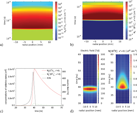
Figure 12. Radial and temporal 2D concentrations of N2(C , v
, v ) (a) and N
 (B
(B , v
, v ) (b) induced by the reduced electric field distribution in the streamer head (see figure 10) generated in synthetic air at 4 torr. For the axial position of r = 0 mm the electric field is shown for comparison in panel (c). The comparison of the experimentally determined electric field distribution (the same as in figure 10(a)) and resulting computed distribution of N
 (B
(B , v
, v ) state density (i.e. FNS emission, the same data as in panel (b) of this figure) in the streamer head is shown in panel (d). The resolved radial structure in both distributions is apparent.
Download figure:
Standard image High-resolution imageAs can be seen in figure 12(a), the shape of the concentration N2(C3 , v
, v ) resembles the two-dimensional emission of the SPS band at 337.1 nm shown in figure 6(b). Between 30 ns and 41 ns, the main production mechanisms of N2(C3
 , v
, v ) are direct electron impact excitation (e + N2
  N2(C3
N2(C3 , v
, v ) + e) and collisional deactivation of N2(C3
 , v
, v ) by N2 producing N2(C3
 , v
, v ) and N2(X1
 , v = 1). However, the production rate (in cm−3 s−1) via electron impact excitation is three orders of magnitude higher than the collisional deactivation. The principal loss channels of N2(C3
 , v
, v ) are radiative decay to N2(B3
 , v = 0, 1) followed by quenching of N2(C3
 , v
, v ) by O2 producing N2 and O2 or N2 and O + O.
The concentration of N2(C3 , v
, v ) reaches its maximum value at ≃41 ns near the center (r = 0 mm) of the discharge axis (see figure 12(c)). At the borders of the streamer emission (r = −12 mm and 12 mm), the density of N2(C3
 , v
, v ) is slightly reduced since direct electron-impact excitation is less efficient in those regions. At ≃50 ns, the concentration of N2(C3
 , v
, v ) decreases by a factor of two and, at 100 ns and 150 ns, it decreases by, respectively, one and two orders of magnitude with respect to its maximum (peak) value of
  cm−3.
cm−3.
Regarding the concentration of  (B2
(B2 , v
, v ) shown in figure 12(b), direct electron impact ionization from the ground electronic state of N2 (e + N2(X1
 )
) 
 (B2
(B2 , v
, v ) + 2 e) is the dominant production mechanism of
  (B2
(B2 , v
, v ) while quenching (
 (B2
(B2 , v
, v ) + N2 / O2
 (X2
(X2 ) + N2 / O2) and radiative decay (
 (B2
(B2 , v
, v )
) 
 (X2
(X2 ) + 391.5 nm) are the most important loss processes. A significant (>103 cm−3) concentration of
  (B2
(B2 , v
, v ) exists between ≃40 ns and 80 ns for all radial positions.
The time evolution of  (B2
(B2 , v
, v ) and N2(C3
 , v
, v ) are shown in figure 12(c) together with the experimentally determined electric field profile. There, a slight delay of units of nanoseconds between the maxima of both species (and mutually also to the electric field peak) is visible in agreement with previous theoretical and experimental analysis [18, 46].
In panel (d) of the figure 12, the 2D distributions of the experimentally determined electric field and computed  (B2
(B2 , v
, v ) density are shown in linear scale. It gives a clear insight into the FNS emission caused solely by the streamer. The development of this emission in both dimensions, i.e. the radial and the temporal, is well visible. This is comparable with the results of theoretical simulation for similar pressure as shown in [46].
The qualitative and quantitative behaviour of N2(C3 , v
, v ) found in the present measurements in the laboratory agrees with the temporal trend exhibited by the concentration of the (vibrationally) lumped N2(C3
 ) shown in the BJ streamer model in [13] at 27 km altitude. However, no observations or model results exist up to date concerning the spatial (altitude) and temporal dynamics of the vibrational populations of key electronic states such as N2(C3
 , v'), N2(B3
 , v') and
  (B2
(B2 , v') controlling the optical emissions of BJ and Giant Jets in the stratosphere and mesosphere. There is also no information on how BJs can affect electrical characteristics of the stratosphere such as the electrical conductivity [57] which has been explored for Sprites (another type of TLE occurring in the mesosphere).
The radial and temporal 2D concentrations of the metastables N(2D) and N(2P) are shown in, respectively, figures 13(a) and (b). The concentrations of N(2D) and N(2P) start to be significant at ≃30 ns when the measured streamer electric field is high enough to promote direct electron impact dissociative excitation (e + N2(X1 )
)  N + N(2D) / N(2P) + e) and dissociative recombination of N
 (e + N
 (X2
(X2 )
)  N + N(2D)). The densities of both atomic nitrogen excited states 2D and 2P reach their maximum values (
 cm−3) at ≃41 ns. Then, the generation of N(2D) and N(2P) ceases and their densities begin to decrease, mainly driven by N(2D) / N(2P) + O2
  NO + O followed by the less important N(2D) / N(2P) + N2
  N + N2. At ≃0.16 ms, the concentrations of N(2D) and N(2P) have decreased by, respectively, three and five orders of magnitude.
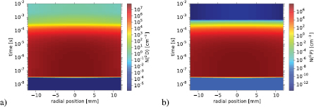
Figure 13. Radial and temporal 2D concentrations of N(2D) (a) and N(2P) (b) induced by the reduced electric field distribution in the streamer head (see figure 10) generated in synthetic air at 4 torr.
Download figure:
Standard image High-resolution imageThe radial and temporal evolution of NO is shown in figure 14. A very important (eight orders of magnitude) increase of NO is produced in a relatively short period of time: between ≃3.5 ns and ≃15 μs. Then, from ≃15 μs to 10 ms, the concentration of NO only increases by less than a factor of two. The kinetic mechanisms underlying the strong and fast increase of NO up to ≃15 μs are N(2D) / N(2P) + O2  NO + O fueled by the N(2D) and N(2P) produced through the (electric field driven) electron-impact dissociative excitation of N2. For times beyond ≃15 μs, the production of NO is controlled by less efficient processes such as N + O2
  NO + O followed by O
 + N2
+ N2  NO + NO+ while, simultaneously, the relative importance of NO loss mechanisms such as O + NO
  NO2, O3 + NO
  O2 + NO2 and O
 + NO
+ NO  O2 + NO+ increases. The trend followed by the NO density suggests that, as predicted by the BJ chemical model in [13], the concentration of NO produced by BJ streamers will slowly decrease for longer (hundreds of ms) times not accessible in the present experiment.
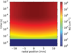
Figure 14. Radial and temporal 2D concentrations of NO induced by the reduced electric field distribution in the streamer head (see figure 10) generated in synthetic air at 4 torr.
Download figure:
Standard image High-resolution imageIt is worth mentioning that the experimental trends found for the concentrations of N(2D), N(2P) and NO are very similar to those predicted by the BJ chemical model in [13]. In addition, the radial and temporal 2D concentrations (not shown) of other nitrogen oxides (NO2, NO3 and N2O) hardly change when computed with the streamer electric field measured in the present experiment.
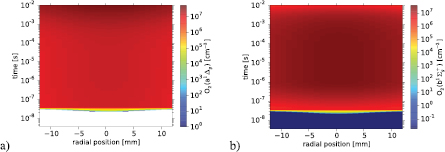
The analysis of the generation or loss of ozone (O3) in BJs is important because BJs take place in the altitude range (the stratosphere of the Earth) where the natural ozone layer is located (around 35 km). The ozone layer protects life on the Earth's surface from damaging solar UV radiation. Therefore, changes in the stratospheric chemical composition due to electrical activity could affect the ambient concentration of O3 with potential effects on the levels of solar UV radiation reaching the surface of the Earth.
The radial and temporal concentration of O3 (not shown) induced by the experimentally derived reduced electric field distribution in laboratory produced streamer heads in synthetic air at 4 torr is found to be negligible. The temporal dependence of the O3 densities computed at three separate radial positions (center and borders) in the discharge reactor is discussed below. A very slight decrease (≃0.05%) is seen with respect to the initial (ambient) ozone values in the reactor up to ≃1 ms, in agreement with a recent BJ chemical model [13].
At the beginning (≃40 ns) of the simulation, the total (sum of the contribution of all considered production or loss mechanisms) formation and removal rates of O3 were  cm−3 s−1 and
  cm−3 s−1, respectively. At 10 ms (when our computations stop), the total formation and removal rates changed to, respectively,
  cm−3 s−1 and
  cm−3 s−1, that is, while the total formation has increased by a factor of three, the total removal rate has decreased almost three orders of magnitude. Thus, during the 10 ms of our computations using measured electric fields up to ≃40 ns, the concentration of O3 remains flat, unaffected by the presence of the electric discharge. However, according to the above mentioned trends of the total formation and removal rates of O3, the density of O3 might slightly increase for longer times (>10 ms), as pointed out in [13]. At 4 torr (37 km altitude) the calculated variation of O3 for relatively long times (tens of seconds) is negligible (less than 5 per cent). At higher pressures (lower altitudes) BJ seem to be able to increase the amount of O3 by a factor of two at 20 km altitude [13].
Among the 17 considered gain mechanisms of O3, the dominant ones at ≃40 ns are, in order of importance, O + O2 + N2 / O2  O3 + N2 / O2 followed by O− + O2
  O3 + e. Also, the key O3 removal processes (among the 21 considered) are e + O3
  O2 + 2 O, e + O3
  O− + O2 and O(1D) + O3
  2 O2 / 2 O + O2.
It is also worth noting that at 10 ms (when NO reaches its hightest value), the contribution of the kinetic path NO + O3  O2 + NO2 to the destruction of O3 is modest, being the eighth (out of a total of 21) most important loss process, after (in order of importance) e + O3
  O2 + 2 O,
  + O3
+ O3  3 O2 + e,
  + O3
+ O3  O2 +
O2 +  , O2(b1
 ) + O3
  2 O2(a1
 ) + O, e + O3
  O− + O2, O + O3
  2 O2 and NO
 + O3
+ O3  O2 + NO
 .
.
Figure 15 shows the radial and temporal 2D concentrations of the metastable O(1D) (a) and ground atomic oxygen O (b) calculated with the measured streamer electric field. The species O(1D) plays a role in the early time (up to 1 ms) slight removal (O(1D) + O3  2 O2 / 2 O + O2) of O3 while the ground state atomic oxygen is involved in the dominant mechanisms (O + O2 + N2 / O2
  O3 + N2 / O2) generating O3 that become increasingly important as the density of atomic oxygen grows (see figure 15(b)).
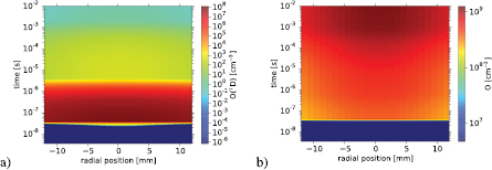
Figure 15. Radial and temporal 2D concentrations of the metastable O(1D) (a) and ground atomic oxygen O (b) induced by the reduced electric field distribution in the streamer head (see figure 10) generated in synthetic air at 4 torr.
Download figure:
Standard image High-resolution imageLastly, figure 16 shows the variations in time and radial position of the concentration of the metastable electronic states a1 and b1
 of O2. These two O2 metastable states are important because, due to their long radiative lifetime, they can transfer energy to the surrounding atmosphere by fast quenching. The ambient (before the discharge begins) concentrations of both O2(b1
 ) and O2(a1
 ) are rather small but, as the the electron density grows by electron-impact ionization (driven by the streamer electric field), they also grow very rapidly up to relatively high values (≃107 cm−3). In this way, the concentration of O2(a1
 ) is controlled by e + O2
  O2(a1
O2(a1 ) + e up to ≃41 ns. Then, between ≃41 ns and ≃1.5 μs, O(1D) + O2
  O + O2(a1
 ) replaces electron-impact production of O2(a1
 ) and keeps it growing, though its production later is lower and losses (by fast quenching, that is, O2(a1
 ) + O2 / N2
  O2 + O2 / N2) increase. Beyond ≃15 μs, O(1D) + O2
  O + O2(a1
 ) no longer dominates the formation of O2(a1
 ) and it is replaced by (in order of importance) O2(b
 ) + N2
  O2(a
O2(a ) + N2, O2(b
 ) + O3
  O2(a
O2(a ) + O3 and O2(b1
 ) + O2
  O2(a
O2(a ) + O2.
Figure 16. Radial and temporal 2D concentrations of the metastables O2(a ) (a) and O2(b
 ) (b) induced by the reduced electric field distribution in the streamer head (see figure 10) generated in synthetic air at 4 torr.
Download figure:
Standard image High-resolution image
The concentration of O2(b ) reaches its maximum at ≃2.2 μs and, after that time, fast quenching of O2(b
 ) by N2, O3 and O2 dominate and produce O2(a
 ).
).
6. Summary and conclusions
In this paper we report the determination of the spatiotemporally resolved distribution of the electric field in streamer heads at a pressure of 4 torr in synthetic air. This result is based on experimental measurements of mono-filamentary non-branched positive streamers periodically produced in a volume point-to-plane DBD electrode geometry. Applying a complex 2D fitting and Abel inversion procedures on the projected and sequentially scanned SPS and FNS luminosity waveforms, the radially resolved emission intensities were obtained with sub-nanosecond temporal resolution. The E/N is determined from the ratio of FNS/SPS intensities. The resulting axially-symmetric reduced electric field strength distribution peaks at 500 Td, with a temporal profile corresponding to the theoretical results on streamer structure by Kulikovsky [52], which is also used as a tool for extrapolation to low field values. The influence of the different sets of quenching constant on the resulting electric field strength is presented on sub-nanosecond resolved data for the first time. We point out that applying the above mentioned method of electric field determination, the use of different quenching sets can result in reduced electric field values differing by a factor of almost two (a peak value of 500 Td for quenching constants from [37] and 950 Td for [55]).
The obtained highly-resolved electric field pattern can serve as a benchmark for kinetic modelling of the plasma chemistry in streamer discharges, e.g. for validating the models of streamer phenomena in the upper atmosphere of the Earth. Here, we used the experimentally obtained reduced electric field strength profiles of low pressure laboratory produced streamers as an input to a kinetic model [11, 58–60] in order to investigate how the streamer phase of Blue Jets affects the stratospheric air plasma chemistry. As a result, the 2D density distributions of important chemical species induced in the streamer heads have been calculated. In particular, we have investigated electrons, the excited electronic states N2(C3 , v
, v ) and
) and  (B2
(B2 , v
, v ), nitrogen atomic metastables N(2D) and N(2P), NO and ozone, atomic oxygen metastable O(1D) and ground state O, metastables O2(a1
 ) and O2(b1
 ). The production of ozone was found to be negligible while that of nitride oxide (NO) was considerably enhanced with respect to its ambient value.
We found that streamers produced under low pressure conditions (4 torr or 37 km altitude) are able to seed the air ahead BJs with significant transient concentrations of chemical species such as O(1D) and N(2D) that contribute to fast heating and, ultimately, to the streamer to leader transition.
In general, the concentration of all the above mentioned chemical species are qualitatively consistent and support the findings of recent models [13] that study the local chemical influence of Blue Jet streamers in the stratosphere even though those models (i.e. [13]) only use simplified synthetic electric field pulses.
As the conditions in the upper atmosphere differ not only in the pressure, additional experimental efforts as well as an extension of the spectral analysis into the VIS-NIR spectral range are necessary.
Acknowledgments
This research was funded by the Academy of Sciences of the Czech Republic under collaborative project M100431201 between the IPP Prague and IAA Granada. TH was supported through the European Science Foundation within the network entitled 'Thunderstorm effects on the atmosphere-ionosphere system (TEA-IS)' (exchange grant no. 4219). FJGV acknowledges the support of the Spanish Ministry of Science and Innovation, MINECO under projects ESP2013-48032-C5-5-R and ESP2015-69909-C5-2-R. ZB acknowledges the support of the Czech Science Foundation (GACR contract no. 15-04023S).