


ABSTRACT
We present a multiwavelength study of the 2012 March 5 solar eruptive event, with an emphasis on the radio triangulation of the associated radio bursts. The main points of the study are reconstruction of the propagation of shock waves driven by coronal mass ejections (CMEs) using radio observations and finding the relative positions of the CME, the CME-driven shock wave, and its radio signatures. For the first time, radio triangulation is applied to different types of radio bursts in the same event and performed in a detailed way using goniopolarimetric observations from STEREO/Waves and WIND/Waves spacecraft. The event on 2012 March 5 was associated with a X1.1 flare from the NOAA AR 1429 situated near the northeast limb, accompanied by a full halo CME and a radio event comprising long-lasting interplanetary type II radio bursts. The results of the three-dimensional reconstruction of the CME (using SOHO/LASCO, STEREO COR, and HI observations), and modeling with the ENLIL cone model suggest that the CME-driven shock wave arrived at 1 AU at about 12:00 UT on March 7 (as observed by SOHO/CELIAS). The results of radio triangulation show that the source of the type II radio burst was situated on the southern flank of the CME. We suggest that the interaction of the shock wave and a nearby coronal streamer resulted in the interplanetary type II radio emission.
Export citation and abstract BibTeX RIS
1. INTRODUCTION
Eruptive processes on the Sun, such as flares and coronal mass ejections (CMEs), are often related to the formation of large-scale disturbances, such as shock waves, that travel through the corona and interplanetary space and can have a significant impact on Earth. Electrons accelerated at propagating shock waves radiate at the local plasma frequency or its harmonics and can be observed in a dynamic spectrum as a so-called type II radio emission (e.g., Wild 1950; Nelson & Melrose 1985; Vršnak & Cliver 2008; Nindos et al. 2008). Metric type II bursts, which appear typically at or below 100 MHz, are caused by shocks traveling through the low solar corona, whereas those recorded in the decameter and kilometer wavelength range are excited by shocks traveling through the upper corona and interplanetary space. The arrival time of CME-driven disturbances to Earth can therefore be estimated using type II radio bursts (e.g., Cremades et al. 2007 and references therein).
It is generally accepted that the majority of interplanetary shocks (within 1 AU) are CME-driven (e.g., Cane et al. 1987; Gopalswamy et al. 2000). However, the relative position of the CME and the associated shock wave and its radio signatures (type II radio bursts) is still a subject of open debate. The majority of studies performed so far are focused on metric type II radio bursts (e.g., Magdalenić et al. 2008; Pohjolainen 2008; Magdalenić et al. 2010; Kerdraon et al. 2010; Nindos et al. 2011; Zimovets et al. 2012), which is explained by the lack of radio imaging in the interplanetary range.
The studies of CMEs and associated shock waves show that metric type II radio bursts mostly appear far from the CME leading edge (Gary et al. 1984; Klein et al. 1999), i.e., close to the CME flanks. Maia et al. (2000) studied a rare and, to our knowledge, unique event in which the scenario of a metric type II radio burst generated close to the leading edge of the CME is plausible.
The situation is significantly more complex for interplanetary type II radio bursts due to the lack of radio imaging observations. Additionally, the interplanetary type II radio bursts are usually observed to be patchy and intermittent, i.e., morphologically rather different from the metric type II bursts, which makes the connection between these two frequency ranges difficult or impossible (Reiner et al. 2003, 2001; Cane & Erickson 2005). The evolution of interplanetary type II radio bursts indicates strong association with CMEs: the type II propagation curve and the propagation curve of the projected leading edge of the CME (the nose of the CME) can be well synchronized. On the other hand, some recent case studies indicate that the interplanetary type II radio emission is preferably originating near the CME flanks (e.g., Xie et al. 2012; Feng et al. 2013b; Shen et al. 2013). The high-density streamer regions (often observed close to the CME flanks) are considered to be places with plasma conditions favorable for shock formation (Evans et al. 2008) and the generation of associated radio emission (e.g., Magdalenić et al. 2002; Schmidt & Cairns 2012, 2014). Moreover, Shen et al. (2013) indicates the streamer–shock interaction region is one of the main source regions of the decameter to hectometric type II radio burst. It is also worth noting that CME–CME interactions are sometimes considered to be a source of the continuum-like radio emission following an interplanetary type II burst (Gopalswamy et al. 2001; Gopalswamy 2011). A recent study by Temmer et al. (2014) discusses enhancements in the interplanetary type II radio burst as well as subsequent intense continuum-like radio emission associated with two interacting CMEs. The authors indicate that enhancement of the radio emission is possibly due to the interaction between the shock of the second CME and the streamer-like, post-eruption current sheet formed behind the first CME.
In order to compensate for the lack of spatial information in the interplanetary range, different methods for estimating the source position of the interplanetary radio emission (type III and type II radio bursts) are being developed (e.g., Fainberg et al. 1972; Krupar et al. 2010, 2012; Martínez Oliveros et al. 2012a; Shen et al. 2013). Triangulation measurements (also referred to as direction-finding measurements) from two or more widely separated spacecraft were previously made using radio instruments on the IMP-6, RAE, and Helios spacecraft and on the WIND and Ulysses spacecraft (Fitzenreiter et al. 1977; Weber et al. 1977; Reiner et al. 1998). More recent attempts to estimate the position of type III radio bursts (Reiner et al. 2009; Thejappa et al. 2012) have used the multipoint observations from the WIND and twin STEREO spacecraft. Similarly, using WIND and STEREO observations, Martínez Oliveros et al. (2012b) studied the position of the type II radio burst. They performed radio triangulation by applying eigenvector and singular value decomposition algorithms (Santolík et al. 2012; Krupar et al. 2012; Martínez Oliveros et al. 2012a). The authors studied a short interval of type II radio emission and obtained a rather large spread in type II radio source positions and somewhat inconsistent results regarding the direction of the radio emission. This inconsistency shows in the radio source positions for lower observing frequencies that appear closer to the Sun than the radio source positions for higher observing frequencies, which therefore indicates shock propagation toward the Sun (see Figure 5 in Martínez Oliveros et al. 2012b). The uncertainty in the results might have been induced by the probable simultaneity of type II and type III radio emission during the considered time intervals.
In this paper, we present a study of the CME/flare event on 2012 March 5, the associated shock wave, and its signatures in white light and radio wavelengths. Section 2 describes the CME/flare event (Section 2.1) and the associated radio emission (Section 2.2). Section 3 is devoted to modeling and simulating the event, which includes a three-dimensional (3D) reconstruction of the CME (Section 3.2) and modeling with the ENLIL cone model (Section 3.1). In Section 4 we estimate the position of the type II and type III radio burst and present the first rather extensive radio triangulation study of different types of radio emission associated with the same CME/flare event. The summary and conclusions are listed in Section 5.
2. OBSERVATIONS
2.1. Flare and CME on 2012 March 5
The Geostationary Operational Environmental Satellite (GOES) observations show a complex flare profile (Figure 1(a)) on 2012 March 5. The flare started at 02:30 UT, achieved its first and second (main) local maxima at about 03:00 UT and 04:05 UT, respectively, and ended around 10:00 UT. The flare originated from NOAA AR 1429 (N19° E58°).
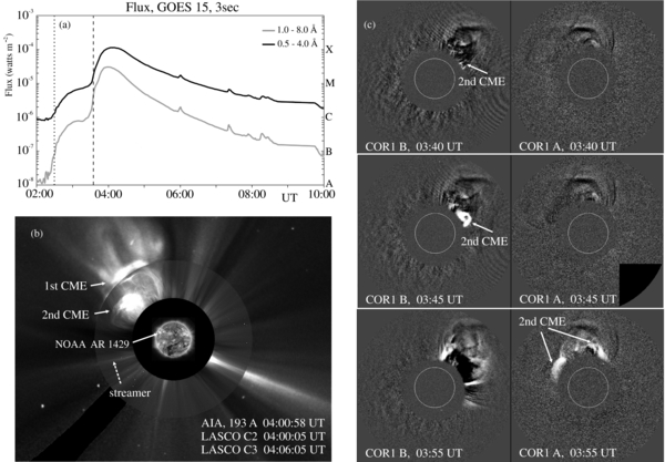
Figure 1. Overview of the CME/flare event. (a) The complex profile of the GOES X1.1 flare gives an indication of possibly two energy releases in progress during the rise time of the flare. The dotted and dashed lines mark the time of the first and second eruption seen in the AIA 171 Å observations. The two eruptions seen in AIA were associated with two CMEs seen by SOHO/LASCO. (b) The combined images of the AIA observations at 193 Å, SOHO/LASCO C2 and SOHO/LASCO C3 observations around 04:00 UT. The observations show two CMEs: the first CME at a height of about 4.7 R☉ and the second CME at 3.9 R☉. (c) The second CME as seen by the STEREO/SECCHI instruments. The left panel presents COR1 B, and the right panel presents COR1 A observations.
Download figure:
Standard image High-resolution imageThe Atmospheric Imaging Assembly (AIA; Lemen et al. 2012) observations from the Solar Dynamics Observatory (SDO) 193 Å passband show two eruptions in NOAA AR 1429 associated with the two GOES flare maxima. The AIA 171 Å observations show coronal loops that slowly start to lift up at 02:00 UT and erupt some 30 minutes later (marked with the dotted line in Figure 1(a)). Hereafter we refer to this ejection, associated with the first flare maxima, as "the first CME". At approximately 03:34 UT the start of the ejection (marked with the dashed line in Figure 1(a)) of a strongly twisted flux rope (hereafter "the second CME") was observed in the same active region. This ejection was associated with the second flare maximum observed at about 04:05 UT.
The event was also observed by the EUV Imagers (EUVI; Howard et al. 2008) on board the Solar TErrestrial RElations Observatory spacecraft (STEREO). The STEREO-Ahead EUVI observations (STEREO-A EUVI) in 304 Å and 195 Å show a weak flare brightening in the northeast quadrant of the Sun. At the same time, STEREO-Behind (STEREO-B EUVI) observed a strong flare brightening in 195 Å and a fast spray-like eruption in 304 Å originating from the active region situated close to the northwest solar limb.
The Large Angle and Spectroscopic COronagraph instruments (LASCO; Brueckner et al. 1995) on board the Solar and Heliospheric Observatory (SOHO; Domingo et al. 1995) also show two CMEs (Figure 1(b)). The first CME appeared in the SOHO/LASCO C2 field of view at 03:12 UT and had a projected speed of 480 km s−1. About one hour later at 04:00 UT, the second full halo CME was observed in the SOHO/LASCO C2 field of view. The second CME had a projected plane-of-the-sky speed of approximately 1230 km s−1 and overtook the first CME in the course of the following 24 minutes (the subsequent SOHO/LASCO C2 image at 04:24 UT shows only one CME).
Both CMEs were seen in the STEREO Sun Earth Connection Coronal and Heliospheric Investigation (STEREO/SECCHI) coronagraphs COR1 and COR2 white-light images. The second CME exhibits a very complex structure in STEREO-A observations; it is difficult to distinguish the trailing structures of the first CME and the leading edge of the second CME. Our study is focused on the second CME (referred to as "the CME" hereafter), first observed in the northwest quadrant of the COR1 B observations at about 03:40 UT and 15 minutes later, 03:55 UT, in COR1 A observations (Figure 1(c)). The Heliospheric Imagers (STEREO/HIs) observations show typically diffused and structured CME with possible signatures of a white-light shock.
Along with the CME, the SOHO/LASCO images also show the presence of a streamer situated close to the southern flank of the CME. The streamer shows a displacement associated with the passage of the CME-driven shock wave. The displacement of the streamer is first observed in the SOHO/LASCO C2 field of view simultaneously with the appearance of the CME itself at 04:00 UT. The white-light shock was most visible, in the SOHO/LASCO C2 field of view, near the southern flank of the CME. The white-light shock will be discussed in more detail in Section 4.2. The displacement of the streamer, associated with the passage of the CME-driven shock wave, was also observed in COR1 B images at 03:55 UT (Figure 1(c)).
2.2. Radio Observations
The radio emission associated with the CME/flare event started at about 03:34 UT with an unusually intense (about 650 000 sfu at 610 MHz) type IV continuum emission in the metric range. The Hiraiso Radiospectrograph (HiRAS; Kondo et al. 1994) observations (Figure 2(a)) show that the drifting continuum emission extends from 50 to 2500 MHz. The dynamic spectrum recorded by the Bruny Island Radio Spectrometer (BIRS; Erickson 1997) shows the continuum emission, a group of low-frequency type III bursts associated with the impulsive phase of the flare and a complex multiple-lane type II emission (marked with arrows in Figure 2(b)).
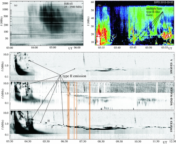
Figure 2. Overview of the radio event. (a) The HiRAS dynamic spectrum shows strong continuum emission probably associated with the CME/flare event. (b) Dynamic spectrum recorded by BIRS shows multiple-lane type II-like burst that consists of short-lived, patchy, and slow-drift emission lanes, low-frequency type III bursts, and type IV continuum emission. (c) The radio emission in DH to km wavelength range. The two top panels show the observations by STEREO/Waves, and the bottom panel is observations by WIND/Waves.
Download figure:
Standard image High-resolution imageThe interplanetary type II emission was observed by the Waves instrument on board the WIND spacecraft (WIND/Waves; Bougeret et al. 1995) and two Waves instruments on board STEREO (STEREO/Waves; Kaiser 2005; Kaiser et al. 2008; Bougeret et al. 2008). The type II burst is a radio signature of a propagating interplanetary shock wave, which is the main subject of this study. Figure 2(c) shows that the radio emissions observed in the metric range, i.e., type III bursts, as well as a multiple-lane type II burst, extend into the decameter to kilometer range. A diffuse and very slowly drifting interplanetary type II-like radio emission was observed after 09:00 UT (Figure 2(c)). The drifting emission appears almost like a continuation of the hectometric type II radio burst but with a slower drift rate.
The STEREO B observations (middle panel of Figure 2(c)) show well-defined, long-lasting, and intense type II radio emission. The intensity of the type II radio burst is somewhat fainter in the WIND observations and very faint in the STEREO A observations (Figure 2(c) bottom and top panel, respectively). If we assume that the radio emission is most intense along the direction of propagation of its source, then we can estimate the direction of the propagation of the CME-driven shock wave and of the CME itself. In this event, we estimate that the shock wave and the CME are propagating between the STEREO B and WIND spacecraft, with the direction somewhat more toward STEREO B. We note that the "intensity–directivity relation" is more exact for STEREO observations because for the comparison with WIND data a somewhat different sensitivity of the antenna should be accounted for. This relation of the intensity and directivity of the type II emission is observed for more events and will be addressed in a separate publication (J. Magdalenić et al., in preparation).
To derive the velocity of the type II burst, we used the frequency drift of the type II radio burst and the Saito (1970) coronal electron density model in the metric range and the Leblanc et al. (1998) electron density model for the decametric to kilometric range. We used five-fold Saito (1970) and one-fold Leblanc et al. (1998) density models and obtained shock speeds of about 1900 km s−1 and 700 km s−1 in the metric and decametric to kilometric range, respectively. The selected electron density models are generally considered suitable for complex flaring events. Similar shock speeds were obtained (1830 km s−1 in the metric and 900 km s−1 in the decametric to kilometric range) while using the hybrid electron density model by Vršnak et al. (2004), which is applicable for the whole range of distances. We note that the shock speed did not differ significantly when estimated using observations from different spacecraft, i.e., STEREO B and WIND observations.
3. MODELING AND SIMULATION OF THE 2012 MARCH 5 EVENT
3.1. 3D Reconstruction of the CME
On March 5, the separation angle between STEREO A and STEREO B was about 133°, and the separation angle between STEREO A and STEREO B with the Earth was 109° and 118°, respectively. This configuration of the spacecraft provided good observations for performing 3D reconstructions of coronal structures like CMEs and streamers (see, e.g., Mierla et al. 2008; Thompson 2013; Feng et al. 2013a).
The two eruptions on March 5 were observed in close temporal succession, but only the second CME seemed to be directly associated with the studied shock wave. Therefore we make the 3D reconstruction only for the second CME. A 3D reconstruction of the CME was made using the graduated cylindrical shell model (Thernisien et al. 2006, 2009; Thernisien 2011), a forward modeling technique for a flux rope-like CME (Chen et al. 1997). This model reproduces the large-scale structure of a flux rope-like CME, modeling only the surface of the CME without rendering its internal structure. The model consists of a tubular section forming the main body of the CME attached to two cones that correspond to the "legs" of the CME. Because of the rather simple structure of the model, the reconstruction gives information mostly on the propagation of the leading edge of the CME.
The trailing structures of the first CME visible in the coronagraph data made the 3D reconstruction of the second CME, using the simple flux rope model, quite difficult to perform. We therefore note that the CME reconstruction gives a rather conservative representation of the CME and that the extent and the width of the CME were probably larger than those obtained with the reconstruction. Figure 3 shows the reconstructed flux rope (green-grid croissant) on SOHO/LASCO and STEREO/SECCHI COR images. Results of the 3D reconstruction enabled a rather accurate estimation of the CME speed. The 3D speeds of the radial CME propagation in the STEREO COR1 and COR2 fields of view were found to be 1370 km s−1 and 1020 km s−1, respectively.

Figure 3. 3D reconstruction of the CME in the SOHO/LASCO C2 and STEREO/SECCHI COR1 field of view and in the SOHO/LASCO C3 and STEREO/SECCHI COR2 field of view (top and bottom panels, respectively). The reconstructed flux rope is denoted with the green grid croissant.
Download figure:
Standard image High-resolution imageThe 3D reconstruction of the CME was not possible in the STEREO HI (Howard et al. 2008) field of view (>15R☉) because of the very diffuse structure of the CME and its leading edge at these heights. The CME speed of about 740 km s−1 in the HI field of view was obtained using the Point-P and FixedPhi methods (Rouillard et al. 2008). Figure 4(a) shows the kinematics of the projected leading edge of the CME obtained with the 3D reconstruction of the CME and the Point-P and FixedPhi methods. The CME velocity between the HI field of view and the shock-like structure at 1 AU (as observed by the CELIAS/MTOF Proton Monitor on SOHO) was obtained as a linear fit (Figure 4(b)).
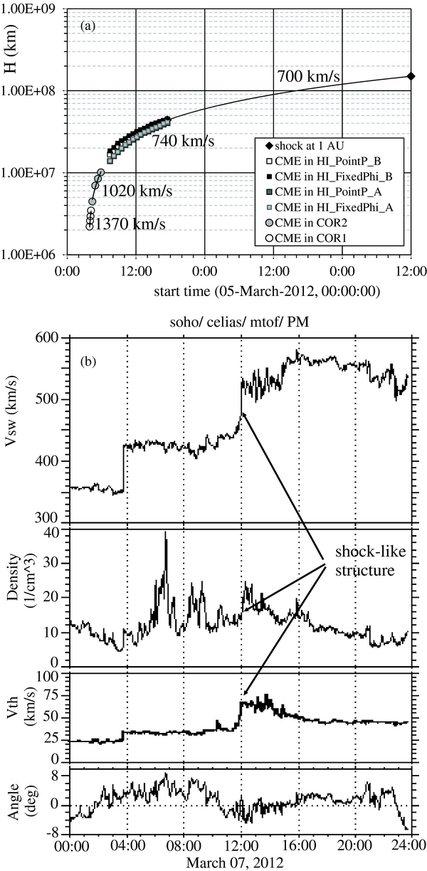
Figure 4. (a) Kinematics of the projected leading edge of the CME is presented. The CME speeds are 3D speeds of the radial propagation obtained from the 3D reconstruction in COR1 and COR2 fields of view and with the Point-P and FixedPhi methods in the HI field of view. The speed of the CME beyond the HI field of view is a linear fit between the points obtained in the HI field of view and arrival of the shock-like structure at 1 AU, as observed by CELIAS/MTOF Proton Monitor on SOHO. (b) The SOHO/CELIAS/MTOF data show arrival of the shock-like structure at 12:00 UT on 2012 March 7.
Download figure:
Standard image High-resolution image3.2. The ENLIL Cone Model
The SOHO and STEREO observations (Figure 3) show that the bulk of the CME mass was directed northward of the Sun–Earth line and that only the arrival of the CME-driven shock wave was expected at Earth. The observations from the CELIAS/MTOF Proton Monitor on SOHO show a shock-like structure at 12:00 UT on March 7 (Figure 4(b)), possibly associated with the second CME from March 5. The discontinuity-like feature was observed in the solar wind speed, proton density, and thermal speed. However, because the observations from the Advanced Composition Explorer spacecraft ACE were corrupted due to an ongoing particle event (associated with a halo CME that erupted on March 4), it was not possible to confirm that the discontinuity-like feature observed in the SOHO/CELIAS data was a signature of a shock wave. Therefore, the motivation for this part of the study was to understand if there is an association between the second CME and the shock-like structure in the SOHO/CELIAS/MTOF data.
In order to investigate the 3D evolution of the second CME in interplanetary space and confirm the possible arrival of the CME at Earth, we used the ENLIL cone model (e.g., Odstrčil et al. 1996; Odstrčil & Pizzo 1999; Odstrčil et al. 2005; Xie et al. 2004). The ENLIL cone model is a time-dependent 3D MHD model of the heliosphere. The model calculates the time-dependent behavior of the ideal fluid due to various initial and boundary conditions. It forecasts CME propagation from the inner radial boundary (which is either at 21.5 R☉ or 30.0 R☉) to the point of interest. The background solar wind used in the ENLIL cone model is based on the Wang–Sheeley–Arge solar wind model (e.g., Arge & Pizzo 2000; Arge et al. 2004). The runs of the ENLIL cone model are done through the Community Coordinated Modeling Center (CCMC, see http://ccmc.gsfc.nasa.gov/).
The CME parameters (cone latitude, cone longitude, and cone angular width) obtained from the CME reconstruction described in Section 3.1 and the CME speed at 21.5 R☉ were used as inputs to the ENLIL model. The ENLIL cone model predicted the CME arrival time at Earth (1 AU) to be 08:34 ± 7 hr on 2012 March 7. Figure 5 shows the simulation results as 2D density contours in the ecliptic and meridian planes (left and middle panel, respectively) on March 7. The model also predicts that the CME should not hit STEREO-B or that the impact should be very weak. The observations indeed show a shock-like structure in the STEREO-B data (18:00 UT on March 7). The arrival time at 1 AU obtained from modeling corresponds well, within the error of prediction, with the shock-like structure observed in the SOHO/CELIAS/MTOF data at 12:00 UT on 2012 March 7. Therefore, we conclude that it is very likely that this shock-like structure is associated with the second CME observed in the coronagraph images on March 5. We note that the observations of CME-driven shock-like structures that do not steepen into classical shocks are not uncommon (e.g., Skoug et al. 1999).
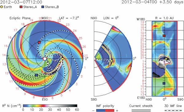
Figure 5. Snapshot of the ENLIL cone model simulation for the 2012 March 5 event. The 2D density contours in the ecliptic and meridian plane (left and middle panel, respectively) and R = 1 AU surface (right panel) are shown for 12:00 UT, the time of arrival of the shock-like structure in the SOHO/CELIAS/MTOF data. The model predicts the CME arrival at Earth at 08:34 ± 7 hr.
Download figure:
Standard image High-resolution imageAlthough the ENLIL cone model does not distinguish between the CME body and the CME-driven shock wave, it can provide an indication of the possible interaction of the CME/shock wave and the streamer. The displacement of the streamer associated with the passage of the CME-driven shock wave in this event was first observed at low heights, i.e., shortly after the first appearance of the CME in the field of view of the COR1 B coronagraph (Figure 1(c)). Therefore, the ENLIL cone model simulations cannot provide an indication of the first interaction of the streamer and the CME but only the streamer–CME interaction at heights above 21.5R☉ (the lowest height of the ENLIL cone model simulation; see Figure 6). The first two panels of Figure 6 show synoptic maps of the magnetic field and the particle number density, scaled with the radial distance. A well-defined magnetic neutral line (Figure 6(a) coincides with the dense streamer seen in the density synoptic map (Figure 6(b)). The subsequent image at 12:02:03 UT (time resolution of the simulation is six hours) shows the modeled CME between Carrington longitudes 75° and 215°, partially situated in a region previously occupied by a streamer, thus giving an indication of their interaction. We note that the position of the streamer obtained from a 3D reconstruction roughly corresponds to the streamer position obtained with the ENLIL model (Carrington longitude about 110° and Carrington latitude of about 40°).
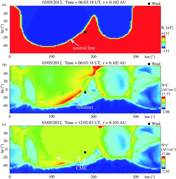
Figure 6. (a) Synoptic map of the magnetic field (scaled with the radial distance) in the high corona. The map is the output of the ENLIL cone model simulation for the 2012 March 5 event. The considered radial distance is 0.102 AU, the lowest height of the ENLIL cone model simulation. (b and c) Synoptic maps of the particle number density (scaled with the radial distance) obtained from the ENLIL cone model simulation (r = 0.102 AU). Two maps show the streamer and CME at 06:03:18 UT and 12:02:03 UT, panels (b) and (c), respectively. The black square represents the WIND spacecraft.
Download figure:
Standard image High-resolution image4. RADIO TRIANGULATION
In this study we used the radio triangulation measurements, also often called direction-finding or goniopolarimetric observations, from WIND and STEREO spacecraft. The direction of arrival of an incoming electromagnetic radio wave, its flux, and its polarization can be derived from these observations. Because of the different types of antenna on these spacecraft, we applied different direction-finding methods. For the WIND observations we used the standard spinning demodulation method described in Manning & Fainberg (1980). For the STEREO B observations we applied a recently developed goniopolarimetric inversion of a signal measured on nonorthogonal antennas using the singular value decomposition (SVD) technique (Krupar et al. 2012). This technique enabled the determination of the wave vector directions, polarization properties, and angular half apertures of apparent source sizes (γ) of the incident waves.
In this direction-finding study we retrieved the wave vector directions, which allowed us to estimate the radio source location for a case when radio emission is observed by two or more spacecraft. The position of the radio source in the 3D space is then considered to be the closest point between the two wave vectors (Krupar et al. 2013, 2014). The shortest distance between wave vectors gives an indication of the error of the source position. We call the described method radio triangulation.
The results of the recent statistical study by Krupar et al. (2013, 2014) indicate that the type III radio source positions obtained by radio triangulation are most reliable at frequencies above 400 kHz because for lower frequencies apparent source sizes seem to be very extended (γ ∼ 50°). A possible explanation for this finding is the strong influence of the scattering of the radio beams at low frequencies (Melrose 1970; Thejappa et al. 2007). Therefore, we consider only frequencies above 400 kHz in this study. Because the interplanetary type II radio emission is usually intermittent and of variable intensity (Vršnak et al. 2001), we applied background subtraction of the lowest five percent of the signal.
In general, several sources of error can influence the direction-finding measurements and consequently also the results of the radio triangulation (see, e.g., Cecconi et al. 2008 and references therein). Here we list only the most obvious characteristics of goniopolarimetric observations that are the sources of uncertainty in the estimation of the position of radio bursts. First, the accuracy of the radio triangulation depends on the separation angle between the spacecraft, with the angle of 90° as the most favorable one (Bougeret et al. 2008). Second, the width of the observing frequency channel, i.e., the effective bandwidth, differs between the used receivers (3 kHz for WIND and 25 kHz for STEREO). Further on, the goniopolarimetric observations are made for a selected set of frequency channels at each spacecraft, and the observing frequencies differ slightly for WIND and STEREO observations (Bougeret et al. 1995, 2008), which also induces some uncertainty in the source position estimation. However, Krupar et al. (2012) report that the largest source of error in estimation of the wave vector direction and apparent source size for the STEREO instruments is the uncertainty in the receiver gain.
4.1. Source Positions of the Type III Radio Burst
To test the accuracy of the method described above, we first performed the radio triangulation of a well-defined type III radio burst, observed at about 03:50 UT on March 5, using observations from all three spacecraft, WIND and both STEREOs (Figure 2).
The radio triangulation is made using simultaneous goniopolarimetric measurements from two spacecraft. Therefore, when the radio signal is well observed by all three spacecraft, the radio triangulation can be made for three different pairs of observations. We performed the radio triangulation for all three pairs of observations using the frequency pair 625/624 kHz (see Figure 7). This frequency pair was selected because the frequencies differ by only one kHz and the type III radio burst was clearly defined at both frequencies. For this part of the study, we selected points around the local maximum of the type III radio flux. It can be seen in Figure 7 that the spread of the radio source positions is the largest for the triangulation made using the STEREO A and STEREO B observations and smallest when combining STEREO B and WIND observations. The same was observed for the triangulation of the type II burst (see Section 4.2). We note that the results of the radio triangulation seem to be the best (least dispersed) when using the goniopolarimetric observations from the two spacecraft between which the radio source is propagating. This conclusion is in agreement with the above-mentioned hypothesis on the intensity–directivity relation for the radio emission (Section 2.2).

Figure 7. Radio triangulation of the type III radio burst at the frequency pair 625/624 MHz. The yellow circle represents the Sun, green represents WIND, blue STEREO B, and the red circle represents the STEREO A spacecraft. The radio source positions obtained by radio triangulation using STEREO A and STEREO B observations are marked with gray points, and for WIND and STEREO A and WIND and STEREO B with red and blue points, respectively. The gray circular line denotes the ecliptic plane. The minor unit on the axes is 0.1 AU. Panels (a)–(d) present different views of the same reconstruction.
Download figure:
Standard image High-resolution imageBecause the best radio triangulation results were achieved with STEREO B and WIND data, these observations were used in a more extensive study of the type III burst. We considered the frequency pairs 1025/1040, 825/804, 625/624, 575/548, 525/548, 475/484, and 425/428 kHz for the WIND and STEREO B observations, respectively. Figure 8 shows two different views on the reconstructed path of the type III radio burst and the reconstructed flux rope. The frequencies are color coded: the dark-green color corresponds to the highest observing frequency pairs and the light green to the lowest frequencies. It is clear that the type III burst was generated by electrons propagating along the open field lines northward of the CME flux rope.
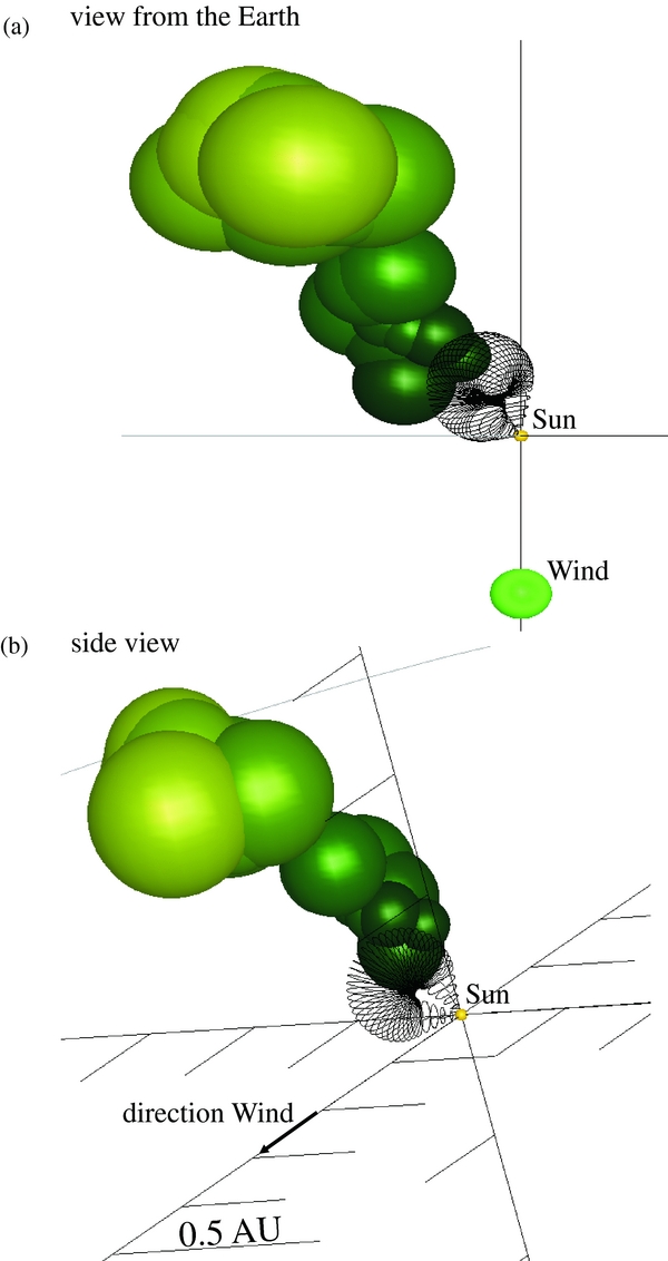
Figure 8. Two different views of the reconstructed propagation path of the type III radio burst. Green spheres represent positions of the type III radio sources obtained with radio triangulation at different frequency pairs. The size of the sphere is a half-distance between the two wave vectors when estimating the source position, and it gives an indication of the uncertainty of the type III source position. Position of the type III radio source is color-coded, where lighter color corresponds to lower observing frequency pairs. The CME flux rope obtained form the 3D reconstruction is presented as a black grid croissant. The large green point represents the WIND satellite and the yellow one represents the Sun.
Download figure:
Standard image High-resolution imageThe size of the sphere that represents the radio sources in Figure 8 is a half-distance between the two wave vectors obtained when estimating the source position. The radio source position is situated within the sphere. The calculated "apparent" source sizes γ increase as the observing frequency decreases, similarly to the increase radio source sizes observed in the metric range.
4.2. Source Positions of the Type II Radio Burst
The STEREO A observations of the interplanetary type II radio burst show low signal-to-noise ratios (see Figures 2(c) and 9(a), two top panels). In addition, results from the radio triangulations of the 625/624 kHz frequency pair, using goniopolarimetric measurements from all three spacecraft, show very dispersed source positions derived from the triangulation of STEREO A with STEREO B and STEREO A with WIND observations. Therefore, for the radio triangulation of the type II emission, we used, as for the type III burst, only WIND and STEREO B observations. We examined five frequency pairs: 625/624, 575/548, 525/548, 475/484, and 425/428 kHz (WIND and STEREO observations, respectively). The criterion for the frequency selection was a well-defined type II radio emission.

Figure 9. (a) Radio flux, colatitude, and azimuth components for STEREO A and STEREO B observations are shown. The radio triangulation was done only for WIND and STEREO B because of low signal-to-noise ratio of STEREO A observations. (b) Top view of reconstructed type II burst sources (orange to gray spheres) together with the reconstructed CME flux rope. The green, red, and blue spheres are the positions of the WIND, STEREO A, and STEREO B spacecraft, respectively.
Download figure:
Standard image High-resolution imageFollowing the procedure for the type III radio burst, we also selected corresponding data points of the type II burst in the STEREO B and WIND data. For the estimation of the type II radio source positions we used three points close to or at the local maximum of the type II radio flux observed by both spacecraft. The points used for the radio triangulation were selected in such a way that intervals of simultaneous type II emission and some other types of radio emission, e.g., weak type III radio bursts, were avoided. In this way we minimized possible ambiguities in the type of radio emission associated with the obtained radio source positions. We show a top view of the reconstructed positions of the type II sources in Figure 9(b) and different views of the reconstructed propagation path of the type II radio burst in Figure 10. The black "cloud" represents the reconstructed CME flux rope expanded self-similarly to the height that the CME reached at the time of the type II radio emission. The yellow sphere represents the position of the Sun, and the orange to gray spheres (higher to lower frequencies, respectively) denote positions of the type II radio source. The green, red, and blue spheres are positions of the WIND, STEREO A, and STEREO B spacecraft, respectively. To highlight the results of the radio triangulation, we present a zoomed view of the reconstructed flux rope and radio sources as seen from Earth in Figure 10(d) and a SOHO/LASCO C3 image showing the CME and the displaced streamer situated close to the southern flank of the CME in Figure 10(e). The shock signature, i.e., type II radio sources, appear close to the southern flank of the CME.
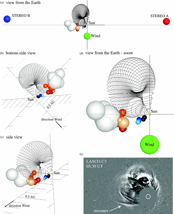
Figure 10. (a–d) Different views of the reconstructed propagation path of the type II radio burst. The CME flux rope obtained from the 3D reconstruction with self-similar expansion is presented as a black grid croissant. The 3D reconstruction of the streamer situated close to the southern flank of the CME is plotted in dark and light blue spheres. The yellow sphere represents the Sun. Panel (d) represents the view of the flux rope and radio sources as seen from Earth. (e) SOHO/LASCO C3 image showing the CME as seen from Earth, for comparison with panel (d).
Download figure:
Standard image High-resolution imageTo visualize the position of the streamer situated close to the flank of the CME in the south solar hemisphere, we applied the tie-pointing method (e.g., Inhester 2006). Figure 10 shows that the reconstructed position of the streamer (denoted with dark blue and light blue spheres) is in close agreement with the direction of the type II radio emission. Therefore, we conclude that the interaction of the shock wave and the streamer most probably resulted in the enhanced type II radio emission.
The heights of the type II radio sources (estimated from the 3D source positions obtained with radio triangulation) were converted to coronal electron densities and plotted in Figure 11 with several other well-known coronal electron density models included for comparison. We note that the fundamental emission band was considered while estimating radio source positions (Figure 2). The top and the bottom of the vertical bars (black spheres) indicate two frequencies of goniopolarimetric observations, and the horizontal bars indicate the full distance between two wave vectors as seen from different spacecraft. We have found that the range of densities obtained using radio triangulation corresponds well with the electron density model of one-fold to two-fold Leblanc et al. (1998). The results obtained for the frequency pair 425/428 kHz show significantly larger distances between two wave vectors than the other considered frequency pairs. Therefore, the density obtained for this frequency pair deviates from the Leblanc et al. (1998) density model. We suggest that this deviation is possibly induced by the scattering of the radio beams at such a low frequency (Melrose 1970; Thejappa et al. 2007).

Figure 11. Coronal electron density/frequency shown as a function of height (in solar radii R☉). The electron density profile obtained from the radio observations is presented with black circles. The position of the radio source at each observing frequency was converted to height. The top and the bottom of the vertical bars (two black circles) indicate two frequencies of goniopolarimetric observations, and the horizontal bars indicate the full distance between two wave vectors as seen from different spacecraft. For comparison, the radial dependence of the plasma density based on the models by Mann et al. (1999), Saito (1970), Leblanc et al. (1998), and Vršnak et al. (2004) is displayed.
Download figure:
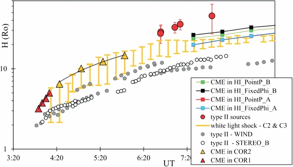
Standard image High-resolution imageFigure 12 summarizes the kinematics of the projected leading edge of the CME (at the CME nose) and the propagation path of the type II burst source obtained from the frequency drift and the coronal electron density model (Leblanc et al. 1998). The extent of the clearly defined white-light shock measured close to the southern flank of the CME in the SOHO/LASCO C2 and C3 fields of view is marked with orange bars. Maximum heights of the visible white-light shock are found to be approximately at the heights of the CME leading edge. The CME nose is seemingly ahead of the shock wave signatures by about 2–5 R☉, indicating that the shock wave might not be CME-driven. On the other hand, the radio source positions of the interplanetary type II burst obtained with the radio triangulation (red circles in Figure 12) are situated about 10–20 R☉ above the CME kinematic curve, which is in agreement with the scenario of a CME-driven shock wave. The discrepancy might be due to the difference between the real and the applied density models and the relative position of the type II radio source and the CME. Indeed, the results of the radio triangulation show that the real corona is somewhat denser than the applied density model (Leblanc et al. 1998) and that the positions of the type II radio source are far from the nose of the CME. The type II radio source is found to be close to the southern flank of the CME. We note that the frequently used presentation of the CME kinematics and shock wave propagation shown in Figure 12 is very informative on the one hand, but on the other it can also be misleading. The reason for the possibly incorrect conclusions based on such a presentation is that the projected heights and projected speeds are considered.
Figure 12. Kinematics of the projected leading edge of the CME at the CME nose and the propagation path of the type II burst sources are shown. Filled gray circles and unfilled black circles show results for WIND and STEREO B obtained using the one-fold Leblanc et al. (1998) coronal electron density model. Red circles show the radio source positions derived from radio triangulation combining WIND and STEREO B observations. The extent of the visible white-light shock, close to the southern flank of the CME, is indicated using yellow bars.
Download figure:
Standard image High-resolution image
5. SUMMARY AND CONCLUSIONS
In this paper we presented a multiwavelength study of the CME/flare event on 2012 March 5. The study is focused on the CME-driven shock wave, with the emphasis on the radio triangulation of the radio emission associated with the event. The first goal of the study was the reconstruction of the propagation of the CME-driven shock wave all the way from the Sun to 1 AU. The second goal of the study was to find the relative positions of the CME, the CME-driven shock wave, and its radio signatures.
The complex X1.1 flare on 2012 March 5 had two maxima associated with two CMEs (Figure 1). We focused on the second full halo CME. The 3D speeds of the radial propagation of the CME were obtained from the 3D reconstruction of the CME (STEREO COR1 and COR2 fields of view) and together with Point-P and FixedPhi methods in the HI field of view. The 3D speeds of the CME are about 11 percent larger than the projected speeds obtained from the SOHO/LASCO observations. The small difference between the projected and 3D speeds is probably due to the direction of the CME propagation close to the plane of the sky.
The kinematics of the projected CME leading edge shown in Figure 4(a) is consistent with the arrival of the shock-like structure at 1 AU on March 7 (as observed by CELIAS/MTOF). Additional confirmation for this association was obtained from the modeling with the ENLIL cone model, which predicted the CME arrival time at Earth at 08:34±7 hr on March 7. The prediction is in good agreement with the arrival of the shock-like structure observed by CELIAS/MTOF at 12:00 UT on March 7 (Figure 4(b)).
The second part of the study was devoted to finding relative positions of the CME, the CME-driven shock wave, and its radio signatures. For this purpose, radio triangulation was employed on the radio emission associated with the CME/flare event. We used goniopolarimetric observations of WIND and two STEREO spacecraft. The radio triangulation of the 2012 March 5 event was performed using the standard spinning demodulation method (Manning & Fainberg 1980) and the singular value decomposition technique (Krupar et al. 2012) for WIND and STEREO observations, respectively. To understand the accuracy and possible limitations of the method, we first applied radio triangulation to the type III radio emission, which generally appears stronger and better defined than more diffuse and patchy type II emission.
Figure 7 shows that the smallest spread in the radio source positions was obtained by radio triangulation when combining STEREO B and WIND observations and largest for the combination of STEREO A and STEREO B observations. Consequently, we reconstructed the propagation path of the fast "type III electrons" using WIND and STEREO B observations. The results of the radio triangulation show that the type III burst was generated by electrons propagating along the open field lines northward of the CME flux rope (Figure 8) and in between WIND and STEREO B spacecraft. These results indicate that the radio source positions obtained from the radio triangulation are most credible when using the goniopolarimetric observations of the two spacecraft between which the source of the radio emission is propagating. It should be noted that this result is in agreement with the hypothesis on the intensity–directivity dependence of the radio emission (see Section 2.2). The study of the type III radio burst showed that the "apparent source size" of the reconstructed sources increase with the decrease in the observing frequency.
For the radio triangulation of the type II burst, we used, like for the type III burst, only WIND and STEREO B observations (see Section 4.2). Figure 11 shows the obtained heights of the type II radio sources converted to coronal electron density and compared with well-known density profiles. The range of densities obtained with the radio triangulation corresponds to the one-fold to two-fold model by Leblanc et al. (1998). The frequency pair 425/428 kHz shows significantly bigger distances between two wave vectors than the other considered frequency pairs and consequently also a certain deviation from the model by Leblanc et al. (1998). This behavior is possibly induced by the scattering of the radio beam at very low frequency (Melrose 1970; Thejappa et al. 2007). We note that the type II and type III burst source sizes obtained in this study (source half-width angle of 20° to 40°) are comparable with the source sizes of type III radio bursts obtained with the same method in the study by Krupar et al. (2012).
The results of radio triangulation show that the source of the type II radio burst was situated southward of the CME nose, i.e., at the southern flank of the CME (Figure 10). This indicates that the interaction of the shock wave and the streamer situated to the south of the CME resulted in the enhanced emission of the interplanetary type II radio burst. The results of the 3D reconstruction of the streamer situated close to the southern flank of the CME in combination with the positions of the type II radio source obtained with radio triangulation and in comparison with the CME position as seen in the SOHO/LASCO C3 image in Figure 10 support the idea of a streamer–shock interaction. This result is in agreement with recent work by Shen et al. (2013), which indicates the streamer–shock interaction region as one of the main source regions of the decameter to hectometric type II radio burst. In addition, the recent study by Floyd et al. (2014) shows that the majority of the bright CMEs are interacting with streamers, which makes the shock–streamer interaction a very probable scenario. However, more events should be analyzed before a general conclusion on the position of the type II source region can be drawn.
The results presented in Figure 12 show that, although this frequently used representation of the CME kinematics and shock wave propagation can be very informative, it can also be misleading because projected heights and projected speeds are used. A well-known source of error can be the application of an inappropriate density model. As shown in this study, the coronal electron density profile for a specific event can differ from the generally considered density profile (Figure 11). In this event, the error in the radio source height introduced by the density model is up to 10 R☉. The second source of the error is the unknown position of the radio emission source with respect to the CME. The radio source may be situated at a CME flank and not at the CME nose as it is often considered (e.g., Gopalswamy et al. 2009).
The results of this study bring new insights into understanding the relative positions of the CME, the CME-driven shock wave, and its radio signatures. In addition, it confirms the great importance of radio triangulation as a method of deriving radio source positions in interplanetary space where radio imaging does not currently exist. In principle, the new ground-based LOFAR (see Van Haarlem et al. 2013) should provide radio imaging observations down to 10 MHz, which is about the limit for ground-based observations. Radio imaging in interplanetary space (kHz range) would demand spacecraft interferometric observations. All of this makes radio triangulation an indispensable method for deriving the radio source positions in interplanetary space.
EIT and LASCO data have been used courtesy of the SOHO/EIT and SOHO/LASCO consortiums, respectively. The CELIAS/MTOF experiment is on the SOHO spacecraft, which is a joint European Space Agency and United States National Aeronautics and Space Administration mission. The STEREO SECCHI data are produced by a consortium of RAL (UK), NRL (USA), LMSAL (USA), GSFC (USA), MPS (Germany), CSL (Belgium), IOTA (France), and IAS (France). The WIND/Waves instrument was designed and built as a joint effort of the Paris-Meudon Observatory, the University of Minnesota, and the Goddard Space Flight Center, and the data are available at the instrument Web site. We are grateful to the staff of the Hiraiso Radiospectrograph and Bruny Island Radio Spectrometer for their open data policy. The simulation carried out for this work was done at the Community Coordinated Modeling Center at NASA Goddard Flight Center. The authors are grateful to M. West for helpful comments. V.K. acknowledges the support of the Czech Grant Agency grant 205-10/2279. A.N.Z. and L.R. acknowledge support from the Belgian Federal Science Policy Office through the ESA-PRODEX program. L.R. partially contributed to the research for the European Union Seventh Framework Programme (FP7/2007-2013) under grant agreement number 263252 [COMESEP]. J.M. and M.M. acknowledge the financial support of Belgian Science Policy (BELSPO) under the Action 1 Programs. This research has been partially funded by the Interuniversity Attraction Poles Programme initiated by the Belgian Science Policy Office (IAP P7/08 CHARM).