Properties of Hall-MHD Turbulence at Sub-Ion Scales: Spectral Transfer Analysis

Abstract

We present results of a multiscale study of Hall-magnetohydrodynamic (MHD) turbulence, carried out on a dataset of compressible nonlinear 2D Hall-MHD numerical simulations of decaying Alfvénic turbulence. For the first time, we identify two distinct regimes of fully developed turbulence. In the first one, the power spectrum of the turbulent magnetic fluctuations at sub-ion scales exhibits a power law with a slope of ∼−2.9, typically observed both in solar wind and in magnetosheath turbulence. The second regime, instead, shows a slope of $-7/3$, in agreement with classical theoretical models of Hall-MHD turbulence. A spectral-transfer analysis reveals that the latter regime occurs when the energy transfer rate at sub-ion scales is dominated by the Hall term, whereas in the former regime, the governing process is the dissipation (and the system exhibits large intermittency). Results of this work are relevant to the space plasma community, as they may potentially reconcile predictions from theoretical models with results from numerical simulations and spacecraft observations.

1. Introduction

Space and astrophysical plasmas are often found in a highly turbulent state. In particular, the solar wind is one of the few natural plasma environments (together with planetary magnetospheres) that is accessible to direct investigation, thanks to space missions and references therein, e.g., [1]. Among others, the turbulent nature of the solar wind is revealed by in situ measurements of the magnetic field. At large scales, where the solar wind behaves as a fluid and can be modeled within the framework of magnetohydrodynamics (MHD), the power spectrum of the magnetic field exhibits a power-law behavior with a spectral index close to $-5/3$ (the so-called inertial range), analogous to the Kolmogorov cascade in hydrodynamic turbulence [2]. When approaching the ion characteristic scales, the spectrum steepens, with a slope ranging from $-2$ to $-4$. The origin of such transition (possibly related to the onset of Hall currents and ion-kinetic dissipation, e.g., [3,4,5]) and the nature of sub-ion scales turbulence are still unknown.

Turbulence properties at sub-ion scales have been the main focus of several studies in the last decades, e.g., [6,7,8,9,10,11,12,13,14,15,16,17]. Early theoretical and numerical studies [7,8,18,19,20] had predicted and/or measured a steepening of the power spectrum to a spectral index of $-7/3$, caused by either the onset of Hall physics or by the change in the wave-like nature of the nonlinear interactions (e.g., kinetic Alfvén waves) that mediate the turbulent energy cascade. Although such slope has been measured in early 3D Hall-MHD numerical simulations, e.g., [21], it was rarely observed by spacecraft [22,23,24]. Instead, a steeper slope with an average value around $-2.8$ or $-3$ is routinely reported, e.g., [25,26], as well as in later numerical studies [4,13,14,16,27,28,29,30]. Refined models incorporating intermittency effects (e.g., assuming that energy dissipation mainly takes place in localized coherent structures such as current sheets [10,31,32] and vorticity structures that form in their vicinity [33,34]) are able to reproduce the ranges of observed slopes. However, there is no definite answer on the nature of the underlying physical mechanisms, nor on the conditions that determine the onset (if any) of different sub-ion scales turbulent regimes.

In this work, we observe the establishment of two different regimes of turbulence at sub-ion scales in 2D compressible viscous-resistive Hall-MHD numerical simulations: (i) the “classic” regime, where turbulence at sub-ion scales is highly intermittent and the magnetic field power spectrum shows a power law with a slope ∼$-2.9$; (ii) a pristine Hall-MHD regime, where the spectral index is $-7/3$. Furthermore, and for the first time, by carrying out a spectral energy transfer analysis [35], we link the appearance of either of the two regimes to specific terms in the equation for the evolution of the energy cascade, one related to the Hall currents, and the other related to dissipation.

The paper is organized as follows. In Section 2, we describe the numerical setup employed and the spectral transfer analysis method. In Section 3, we highlight the general evolution of the Hall-MHD simulations and describe their turbulent spectral properties. Finally, in Section 4, we summarize our results, also in the context of previous works.

2. Methods

2.1. Hall-MHD Simulations of Plasma Turbulence: Numerical Setup

The Hall-MHD model takes into account two-fluid effects generated by the ions decoupling from the electrons and from the magnetic field at scales smaller than the ion inertial length $d_i$. Here, we use a simplified framework: the nonlinear viscous-resistive MHD equations are modified by only adding the Hall term in the induction equation. This is done by substituting the fluid velocity $\mathit{u}$ with the electron velocity ${\mathit{u}}_e=\mathit{u}-\mathit{J}/e{n}_e$, $\mathit{J}$ being the current density, e the unsigned fundamental charge, and $n_e$ the electron numerical density. In their adimensionalized form, the Hall-MHD equations take the form

$$\begin{array}{cc}\hfill {\partial }_t\rho =& -\nabla ·\left(\rho \mathit{u}\right),\hfill \end{array}$$

(1)

$$\begin{array}{cc}\hfill \rho ({\partial }_t+\mathit{u}·\nabla )\mathit{u}=& -\nabla P+(\nabla \times \mathit{B})\times \mathit{B}+\nabla ·\mathbf{\tau },\hfill \end{array}$$

(2)

$$\begin{array}{cc}\hfill ({\partial }_t+\mathit{u}·\nabla )T& =(\mathsf{\Gamma }-1)\left\{{-(\nabla ·\mathit{u})T+\eta |\nabla \times \mathit{B}|}^2/\rho +\mathbf{\tau }:\nabla \mathit{u}/\rho \right\},\hfill \end{array}$$

(3)

$$\begin{array}{cc}\hfill {\partial }_t\mathit{B}=& \nabla \times \left(\mathit{u}\times \mathit{B}\right)+\eta {\nabla }^2\mathit{B}-d_i/L\nabla \times [\mathit{J}\times \mathit{B}/\rho ],\hfill \end{array}$$

(4)

where $\mathit{J}=\nabla \times \mathit{B}$, $\mathbf{\tau }=\mu (\nabla \mathit{u}+\nabla {\mathit{u}}^T-2/3\mathbf{I}\nabla ·\mathit{u})$ is the viscous stress tensor, $\mathsf{\Gamma }=5/3$ is the adiabatic index, and $\{\rho ,\mathit{u},\mathit{B},T,P\}$ denote the usual physical quantities. The pressure evolves according to the equation of state $P=\rho T$. The above equations are normalized with respect to a characteristic length $L=d_i$, a magnetic field amplitude $B_0$, a plasma density ${\rho }_0$, an Alfvén velocity $c_A=B_0/\sqrt{4\pi {\rho }_0}={\mathsf{\Omega }}_i{d}_i$, a pressure $P_0={\rho }_0{c}_A^2$, and a plasma temperature $T_0=k_B{c}_A^2/m_i$. ${\mathsf{\Omega }}_i=e{B}_0/m_{i}c$ denotes the ion-cyclotron frequency and $m_i$ is the mass of the ions. With this normalization, the (adimensional) dynamic viscosity $\mu$ is in units of $d_i{c}_A{\rho }_0$, and the magnetic resistivity $\eta$ is in units of $d_i{c}_A$. Furthermore, we have a plasma $\beta =2P_0/B_0^2=2{\mathsf{\Gamma }}^{-1}{(c_s/c_A)}^2$, where $c_s=\sqrt{\mathsf{\Gamma }{P}_0/{\rho }_0}$ is the adiabatic sound speed. Equations (1)–(4) are numerically solved by means of a pseudospectral 2.5D code [4,36,37,38,39], that evolves the scalar fields $\{\rho ,T\}$ and the 3D vector fields $\{\mathit{u},\mathit{B}\}$ in a 2D $(x,y)$ periodic domain, using Fourier decomposition to calculate spatial derivatives and a third-order Runge–Kutta scheme [40] for temporal integration. In Fourier space, a filter is applied according to the $2/3$ Orszag rule [41], to avoid aliasing of the nonlinear quadratic terms. The aliasing of the nonlinear cubic terms is mitigated by the presence of a finite dissipation [42].

We carry out a series of three numerical simulations of decaying Alfvénic plasma turbulence. For all the simulations, we consider a 2D box of size $L_x\times L_y=32d_i\times 32d_i$ and a grid resolution of $\Delta x=\Delta y=d_i/32$, corresponding to $N_x\times N_y={1024}^2$ points. The system is initialized with a constant ambient magnetic field ${\mathit{B}}_0=B_0{\mathit{e}}_z$ out of the simulation plane, along the z direction (which we name as the parallel direction). The $xy$-plane (i.e., the perpendicular plane) is filled with freely-decaying random (incompressible) Alfvénic-like sinusoidal fluctuations of same amplitude, characterized by a root-mean-square (rms) amplitude $b_{\mathrm{rms}}=u_{\mathrm{rms}}$, a zero mean cross helicity, and wavenumbers spanning from the smallest nonzero value contained in the box up to the injection wavenumber $k_{\perp ,\mathrm{inj}}=2\pi /{\ell }_{\mathrm{inj}}$, where ${\ell }_{\mathrm{inj}}$ is the injection scale and $k_{\perp }=\sqrt{k_x^2+k_y^2}$ (for more details on the initialization, see [14]). Thanks to such initialization, the energy reservoir located above the injection scale is enough to allow the simulations to reach and mantain a fully-developed turbulent state.

In the solar wind, the value of the ion plasma beta ranges from ∼$0.01$ to ∼100, with an average value of 1. If we assume that the electron beta is the same, this translates to a total plasma beta of $\beta =2$. We set this value for the initial plasma beta in all the simulations and we vary the rms of the fluctuations as well as the injection scale and the value of viscosity $\mu$ and resistivity $\eta$ (with $\mu =\eta$).

Table 1. Physical and numerical parameters of the simulations used in this work (in code adimensional units). Box size $L_0$, injection scale $L_{\mathrm{inj}}$, rms amplitude of the initial fluctuations ($b_{\mathrm{rms}}=u_{\mathrm{rms}}$), nonlinear time at the injection scale ${\tau }_{nl}$ (in units of ${\mathsf{\Omega }}_i^{-1}$), viscosity $\mu$ and resistivity $\eta$, (magnetic) Reynolds number $\left(\mathrm{Rm}\right)\mathrm{Re}=L_{\mathrm{inj}}{u}_{\mathrm{rms}}{\rho }_0/\mu$ (since $\mu =\eta$ and ${\rho }_0=1$), and initial Mach number $M_0=u_{\mathrm{rms}}/c_s$. All simulations have the same grid size ($L_{\left[xy\right]}=32d_i$) and resolution ($\Delta \left[xy\right]=d_i/32$). The nonlinear time is defined as ${\tau }_{\mathrm{nl}}=L_{\mathrm{inj}}/u_{\mathrm{rms}}$. $Q_0$ is the total heating rate (in units of ${\rho }_0{c}_A^2{\mathsf{\Omega }}_i$) measured in the time interval of fully developed turbulence considered (see Section 3.2).

Run	${\mathit{L}}_0$	${\mathit{L}}_{\mathbf{inj}}$	${\mathit{u}}_{\mathbf{rms}}\left({\mathit{b}}_{\mathbf{rms}}\right)$	${\mathit{\tau }}_{\mathbf{nl}}$	$\mathit{\mu },\mathit{\eta }$	Re (Rm)	${\mathit{M}}_0$	${\mathit{Q}}_0$
d16	32 $d_i$	16 $d_i$	0.25	64	$5\times {10}^{-4}$	8000	∼$0.19$	$1.8\times {10}^{-4}$
d08a	32 $d_i$	8 $d_i$	0.25	32	$5\times {10}^{-4}$	4000	∼$0.19$	$4.3\times {10}^{-4}$
d08b	32 $d_i$	8 $d_i$	0.30	$26.6$	$2.5\times {10}^{-4}$	9600	∼$0.23$	$7.2\times {10}^{-4}$

reports the simulation dataset used in this work.

2.2. Spectral Transfer Equations

The main property of fully developed turbulence is the onset of an energy cascade. The energy contained in the reservoir at the largest scales is transfered (i.e., “cascades”) to smaller and smaller scales through nonlinear interactions of the fields between nearby spatial scales. In viscoresistive models, such cascade ends at the so-called Kolmogorov scale, where the plasma dynamics is dominated by the dissipation. The total energy transfer rate thoughout all scales results from different terms of different origin. Some terms may be, for example, dominant at large scales and subdominant at small scales, thus determining changes/transitions in the observed plasma regime. In this work, we use the spectral transfer approach [35,43,44] to measure and decompose the energy transfer rate into different contributions. Following [35], the temporal evolution ${\partial }_t(\rho {\mathit{u}}^2+{\mathit{B}}^2)/2$ of kinetic and magnetic energy can be obtained by summing the two inner products of Equations (2) and (4) by $\mathit{u}$ and $\mathit{B}$, respectively. Furthermore, by introducing $\mathit{w}=\sqrt{\rho }\mathit{u}$ [45] and using Parseval’s theorem to transform to Fourier space, we may write

$$\begin{array}{cc}\hfill \frac{{\partial }_t\left(|\overline{\mathit{w}}{|}^2+{\left|\overline{\mathit{B}}\right|}^2\right)}{2}=& -T_{\mathrm{MHD}}-T_{\mathrm{H}}-\Re \left\{{\overline{\mathit{w}}}^{\ast }·\overline{{\rho }^{-1/2}\nabla P}\right\}+\Re \left\{{\overline{\mathit{w}}}^{\ast }·\overline{{\rho }^{-1/2}\nabla ·\mathbf{\tau }}\right\}\hfill \\ \hfill & -\eta k^2{\left|\overline{\mathit{B}}\right|}^2,\hfill \end{array}$$

(5)

where the star denotes the complex conjugate, $\Re \{...\}$ is the real part, wide bars denote the discrete Fourier transform (e.g., $\overline{\mathit{w}}(k_x,k_y,t)={\sum }_{(x,y)}\mathit{w}(x,y,t)e^{-i(k_{x}x+k_{y}y)}/N_x{N}_y$), and each barred quantity is a function of the wave vector $\mathit{k}\equiv {\mathit{k}}_{\perp }=(k_x,k_y)$ and time. The MHD and Hall transfer terms $T_{\mathrm{MHD}}$ and $T_{\mathrm{H}}$ are

$$\begin{array}{c}{T}_{\mathrm{MHD}}=\Re \left\{{\overline{\mathit{w}}}^{\ast }·\left[\overline{\mathit{u}·\nabla \mathit{w}}+\overline{\mathit{w}\nabla ·\mathit{u}}/2-\overline{{\rho }^{-1/2}\mathit{J}\times \mathit{B}}\right]-{\overline{\mathit{B}}}^{\ast }·\overline{\nabla \times \left(\mathit{u}\times \mathit{B}\right)}\right\},\\ T_{\mathrm{H}}=\Re \left\{{\overline{\mathit{B}}}^{\ast }·\overline{\nabla \times \left(\mathit{J}\times \mathit{B}/\rho \right)}\right\}.\end{array}$$

The magnetic+kinetic energy transfer rate from scales with wavenumber smaller or equal to $k=\left|\mathit{k}\right|$ is given by

$${\partial }_t{E}_k=\frac{1}{2}\sum _{|{\mathbf{k}}^{\prime }|\le k}{\partial }_t\left(|\overline{\mathit{w}}{|}^2+{\left|\overline{\mathit{B}}\right|}^2\right)=-S_{\mathrm{MHD},k}-S_{\mathrm{H},k}+{\mathsf{\Psi }}_k-D_k$$

(6)

with

$$\begin{array}{c}{S}_{\mathrm{MHD},k}=\sum _{|{\mathbf{k}}^{\prime }|\le k}{T}_{\mathrm{MHD}},S_{\mathrm{H},k}=\sum _{|{\mathbf{k}}^{\prime }|\le k}{T}_{\mathrm{H}},{\mathsf{\Psi }}_k=-\sum _{|{\mathbf{k}}^{\prime }|\le k}\Re \left\{{\overline{\mathit{w}}}^{\ast }·\overline{{\rho }^{-1/2}\nabla P}\right\},\\ D_k=\sum _{|{\mathbf{k}}^{\prime }|\le k}\left(\eta k^{\prime 2}{\left|\overline{\mathit{B}}\right|}^2-\Re \left\{{\overline{\mathit{w}}}^{\ast }·\overline{{\rho }^{-1/2}\nabla ·\mathbf{\tau }}\right\}\right).\end{array}$$

(7)

In the case of fully developed turbulence (and in general, during the whole evolution [35]), as k increases, we expect to observe a negative energy transfer rate (${\partial }_t{E}_k<0$). Here, $S_{\mathrm{MHD},k}$ and $S_{\mathrm{H},k}$ denote the MHD and the Hall energy transfer term, while ${\mathsf{\Psi }}_k$ and $D_k$ represent the pressure-dilatation and the dissipation term, respectively. The total heating rate $Q_0$, which measures the dissipation of the energy density in the whole domain, correspond to the dissipation rate $D_k$ at the maximum wavenumber. In the following, we will focus on the Hall term and on the dissipation term.

We note that the energy transfer rates introduced in Equation (7) measure a global nonlinear transfer of energy from the sphere of wavectors with radius k. In the case of a turbulent cascade that is local in Fourier space, such energy transfer is the flux through the sphere’s boundary and corresponds to the cascade rate. We also remark that when turbulence is well developed and a cascade is established, the spectral transfer equation is equivalent to the Von Karman–Howarth–Monin equation based on third-order structure functions [35].

3. Results

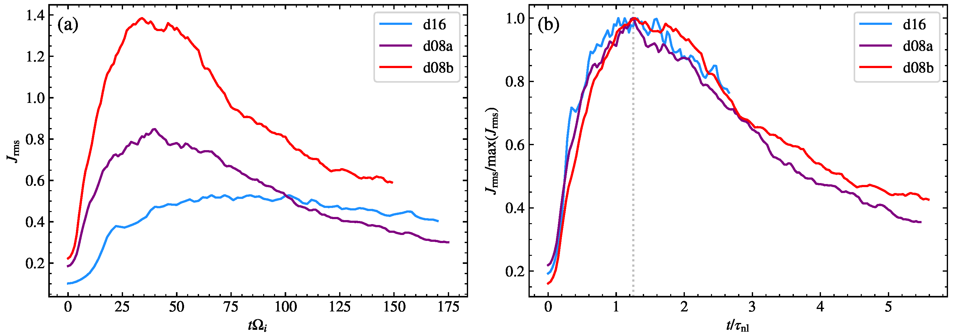
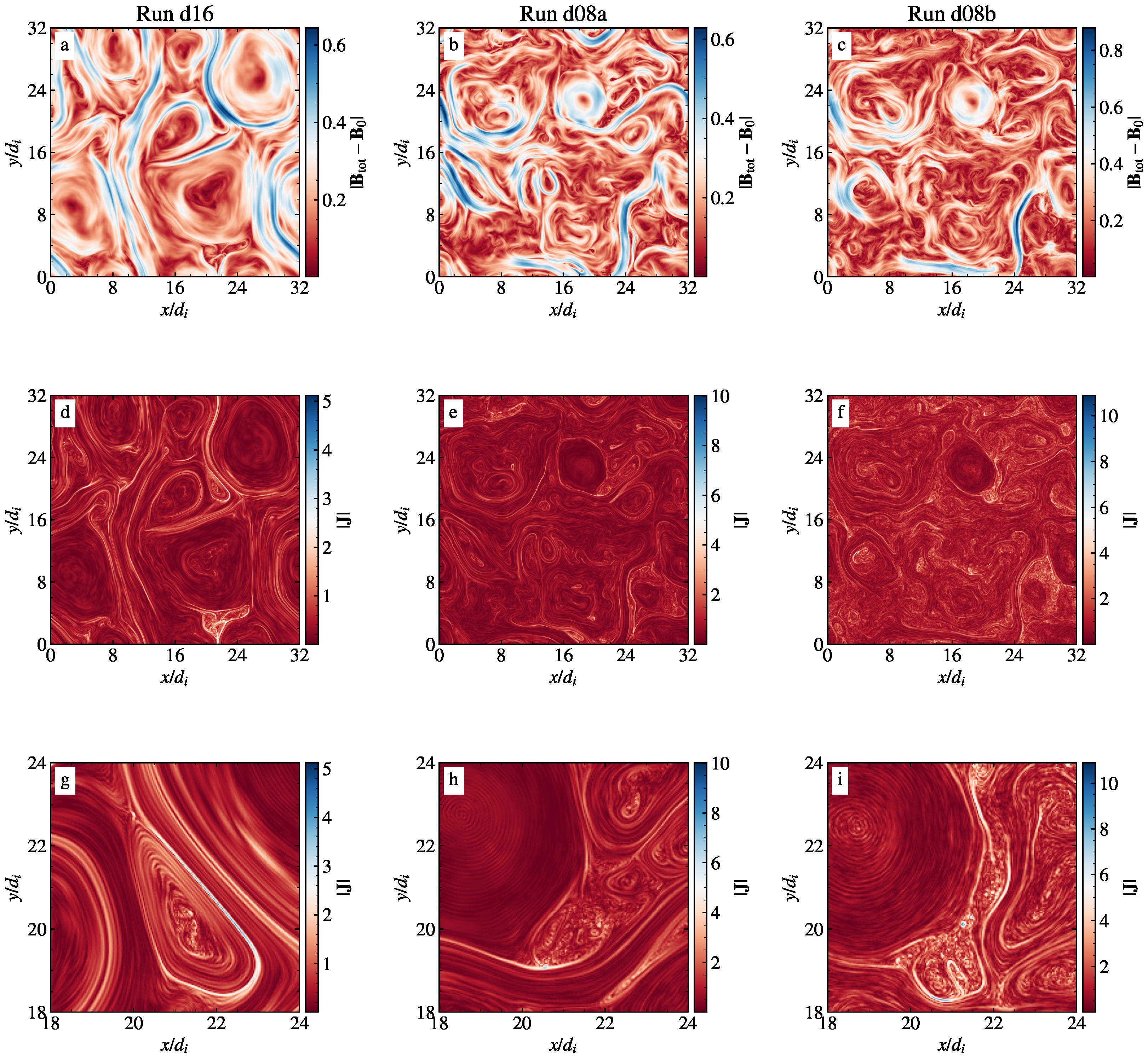
3.1. General Evolution

The overall evolution in the three simulations listed in Table 1 is qualitatively the same. The initial large-scale Alfvénic-like fluctuations quickly evolve to form large vortices and other coherent structures, such as current sheets which then undergo magnetic reconnection. The system then evolves until turbulence has fully developed, corresponding to the maximum of the rms of the current density (for more details on the evolution of a similar setup, see [4]). The time of fully developed turbulence is different for each simulation (as shown in Figure 1). Run d16 takes roughly twice the time of Run d08a(b) to reach the maximum of $J_{\mathrm{rms}}$. This is because the eddy turnover time (also known as the nonlinear time) ${\tau }_{nl}=L_{\mathrm{inj}}/u_{\mathrm{rms}}$ at the injection scale is roughly twice the nonlinear time of the other two runs. Indeed, once we normalize the time with respect to ${\tau }_{nl}$ (see Figure 1b) and $J_{\mathrm{rms}}$ with respect to its maximum, the three curves nicely overlap, with the maximum roughly located at the same time $t=1.25{\tau }_{nl}$ (marked with a vertical dotted line), followed by a plateau, indicating that a statistically quasi-stationary turbulent state (that lasts for $\sim 0.4{\tau }_{nl}$) has been reached and, finally, a slowly decaying phase. We note that the definition of the nonlinear time varies in the literature usually by a constant multiplicative factor of $2\pi$ or by using the size L of the full box instead of the injection scale $L_{\mathrm{inj}}$. However, such constant does not change qualitatively Figure 1b, as it only changes the normalization of the x-axis.

Figure 2 reports, for all three runs, the amplitude of the magnetic field fluctuations (panels a, b, and c) right after the maximum of the turbulent activity has been reached, together with the amplitude of the current density (panels d to i). At large scales, vortices and filamentary structures in both Run d08a and d08b are roughly twice smaller than those in Run d16 (because of the different injection scale). At small scales, the morphological differences between the three runs at sub-ion scales are evident. The filamentary current structures (panels d, e, and g) are more space filling in Run d08a and b and with richer small-scales features (panels g, h, and i), while Run d16 shows more localized and thicker filaments. Finally, compared to Run d08a, the current density in Run d08b is more homogeneously distributed (panels e and f) and with a richer multiscale structure (see panels h and i). This picture was confirmed by measuring the intermittency in the three runs (not shown here). Indeed, high (small) values of intermittency were observed in Run d16 (d08a), while almost no intermittency was observed in Run d08b. The scenario just presented in Figure 2 is consistent with previous works which explored the properties of the dissipative structures that form in 2D, e.g., [17,46,47,48], and 3D [49,50,51] numerical simulations of plasma turbulence.

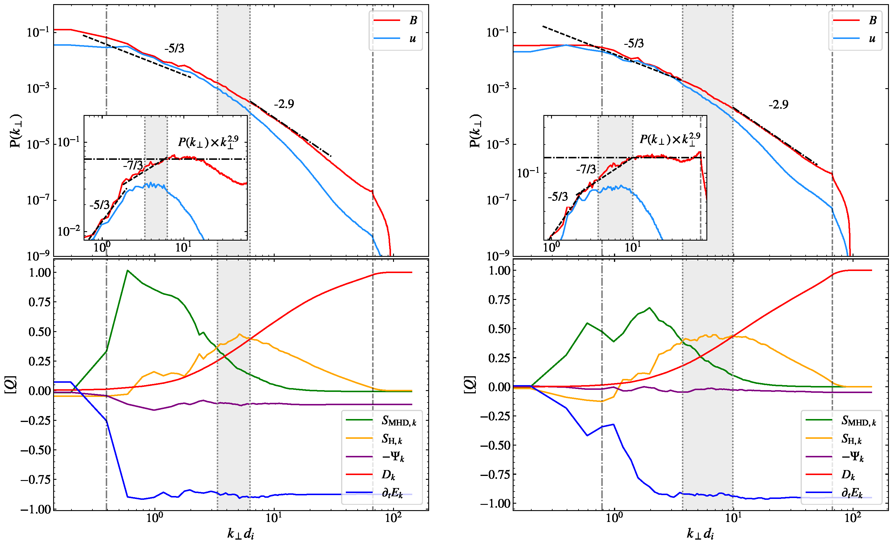
3.2. Spectral Properties and Cross-Scales Energy Transfer

Once turbulence is fully developed, magnetic power spectra of all three runs show well-defined power laws, which last for the entire duration of the plateau and also in the following decaying phase (although the energy decreases). Figure 3 and Figure 4 show the isotropized power spectra [13] (top panels) and the spectral energy transfer (bottom panels) averaged over a time interval of roughly the same length around the plateau, to improve the statistics and decrease the effects of the oscillations in the pressure-dilatation term ${\mathsf{\Psi }}_k$ [35]. The spectral properties of Run d16 are qualitatively the same as those found in our previous works [4,39,48]. We observe the onset of an inertial range cascade of power-law $-5/3$ in the interval $k_{\perp }\in [k_{\perp ,\mathrm{inj}},2]$, followed by a transition to a steeper slope of $-2.9$ in the sub-ion range, shown in the top-left panel of Figure 3. In the inset in the same panel, we report the spectra multiplied by $k_{\perp }^{2.9}$, where we can appreciate the length of the interval of the $-2.9$ slope ($6\lesssim k_{\perp }{d}_i\lesssim 15$). The $-5/3$ and the $-2.9$ power laws are in agreement with those found in our previous works, as well as in other studies [4,13,14,16,28,30]. However, compared to, e.g., Papini et al. [4], here, the transition from the inertial to the sub-ion range is smooth and more extended. Different to that observed in the MHD range in our previous works, the velocity power spectrum in Run d16 (as well as in the other two runs) almost overlaps with the magnetic spectrum, which hints that there is no residual energy present.

The bottom-left panel of Figure 3 shows the spectral energy transfer of Run d16. The behavior is qualitatively similar to that observed by [3,35], but with some important differences. In the inertial range, the MHD term $S_{\mathrm{MHD},k}$ gives the main contribution where we observe the $-5/3$ power law, followed by a small interval in which the MHD, the Hall, and the dissipation term are comparable, with the Hall term $S_{\mathrm{H},k}$ being the largest. This interval ($2\lesssim k_{\perp }{d}_i\lesssim 6$) is the same interval where we observe the smooth transition between the two power laws. In the sub-ion range, the dissipation term $D_k$ dominates, although $S_{\mathrm{H},k}$ still gives a non-negligible contribution. The resulting total energy transfer rate ${\partial }_t{E}_k$ is more or less constant at all wavenumbers above the injection wavenumber.

The top and bottom right panels of Figure 3 show the same plots, except for Run d08a, which differs from Run d16 only in the location of the injection scale, moved further down to $8d_i$ (thus the Reynolds number of Run d08a is half that one of Run d16). In wavenumber, this translates to $k_{\perp ,\mathrm{inj}}{d}_i\sim 0.8$, i.e., at the edge of the ion characteristic scales. As a result, the size of the $-5/3$ MHD inertial range is further shortened. More importantly, the size of the interval where $S_{\mathrm{H},k}$ is the largest term increases, as well as the interval of the transition between the MHD and the sub-ion regimes. Finally, the sub-ion range now shows a more extended $-2.9$ power-law spectrum, almost up to the $2/3$-cutoff wavenumber.

Finally, we consider Run d08b, which has half the resistivity and viscosity of Run d08a and a higher rms of the initial pseudo-Alfvénic fluctuations (see Table 1). This is the most interesting run of this work. Figure 4 shows the power spectrum and the spectral energy transfer of Run d08b. The magnetic power spectrum only shows two power-law regimes. The usual $-5/3$ MHD range, which further extends up to $k_{\perp }{d}_i\sim 4.5$, and a sub-ion range with a clear slope of $-7/3$ (see compensated spectra in the inset) that extends for almost a decade in the interval $k_{\perp }{d}_i\in [4.5,27.4]$ and nicely matches the interval where the Hall energy transfer term is dominant. In such range, the $-7/3$ slope is very stable in time, and lasts up to the end of the simulation, also in the decaying phase and for more than $4{\tau }_{nl}$. Such slope is predicted by theoretical models of Hall-MHD turbulence, but it is rarely measured in spacecraft observations [22,23,24] and it has been only reported in early numerical studies of turbulence, e.g., [20,21].

The concurrent presence of a $-7/3$ slope and of a dominant Hall energy transfer term in Run d08b suggests to reexamine Run d16 and d08a. Indeed, in both runs and in the transition interval between the MHD and the sub-ion range, where $S_{\mathrm{H},k}$ is comparable to $S_{\mathrm{MHD},k}$ and $D_k$, the power spectrum of magnetic fluctuations shows a hint of a $-7/3$ power law (see compensated spectra in the insets in Figure 3).

4. Discussion

The simulation dataset analyzed in this work clearly revealed a strict link between the spectral properties and the spectral energy transfer in Hall-MHD turbulence. Moreover, we have shown that the turbulent cascade at sub-ion scales can enter different regimes depending on which term gives the dominant contribution to the spectral energy transfer rate.

Our interpretation of the different scenarios we reproduced (see Figure 3 and Figure 4) is the following. In the typical case, exemplified by Run d16, the energy injection scales are much larger than the ion characteristic scales; thus, a proper MHD inertial range cascade is established and vortices and coherent structures can form at scales larger than the ion characteristic ones. As a consequence, at sub-ion scales, the cross-scale energy transfer takes place in localized regions of enhanced dissipation. This is in agreement with our previous findings [48] and is coherent with the fact that in Run d16 (and also in other simulations previously analyzed [35]) the dissipation term $D_k$ gives the dominant contribution to the total energy transfer ${\partial }_t{E}_k$. Indeed, in Run d16 we measured high levels of intermittency (not shown here) at sub-ion scales. This does not mean that the Hall term $S_{\mathrm{H},k}$ is unimportant, since the $-2.9$ slope would not form in MHD simulations. Indeed, such slope is present until $D_k\gtrsim 3S_{\mathrm{H},k}$ in both Run d16 and d08a. Instead, in Run d08b the injection scale is so close to the ion characteristic scales that the formation of coherent structures is less efficient, the level of intermittency is very low, and the sub-ion scales turbulence is in a regime where the Hall term $S_{\mathrm{H},k}$ gives the main contribution to the total energy transfer. In this pristine Hall-MHD regime, we observe the $-7/3$ slope, as predicted and observed in previous Hall-MHD studies [18,21]. In particular, we believe that such slope was observed by [21] in their 3D Hall-MHD simulation because the box size was too small to allow for an extended MHD inertial range, which is necessary to develop the intermittency needed for a sub-ion scale regime with $D_k>S_{\mathrm{H},\mathrm{k}}$. Other simulations (not shown in this work), performed by varying the parameters (rms of the fluctuations, resistivity, injection scale, box size), confirm this picture.

Our results are constrained by the 2D geometry, which prevents the onset of 3D intrinsic features of plasma turbulence (e.g., critically balanced turbulence [52]). Indeed, a complete description of plasma turbulence requires the use of 3D modeling, e.g., [53,54]. However, we expect that our results are, to some extent, relevant to a more realistic full 3D case. Indeed, reduced MHD models (that share similarities with the 2.5D MHD description, e.g., [55]) are able to reproduce the turbulent energy dissipation rate at fluid scales [56]. At sub-ion scales, 2.5D models qualitatively capture several properties of turbulent dissipation [46,57]. For instance, spectral turbulent properties in both 2.5D and 3D hybrid-kinetic simulations nicely match, and show remarkable agreement with solar wind observations [58,59]. Finally, our findings obtained with a 2.5D model provide the first explanation for the unfrequent appearence of the $-7/3$ power law in both observations and simulations. Future investigation will assess whether our findings hold in a 3D numerical setup.

In all the simulations presented in this work, we employed a value for the plasma $\beta =2$. The effect of varying the plasma beta on the spectral index of the magnetic power spectra at sub-ion scales has been investigated by [28], who found that the spectral index increases with decreasing plasma beta (as well as the location of the spectral break), with a functional dependence on both the ion inertial length $d_i$ and the ion gyroradius ${\rho }_i$. Unfortunately, the Hall-MHD model does not contain ${\rho }_i$ as a characteristic scale, therefore we are uncertain whether Hall-MHD is able to model the sub-ion scales turbulence at low betas. We will explore this aspect in future works.

We remark the limits of Hall-MHD in properly modeling collisionless plasmas. In particular, it has been shown that the dissipation term in the Von Kármán–Howarth equation (which is equivalent to the spectral transfer approach [35]) cannot properly model hybrid-kinetic simulations of plasma turbulence [3]. However, it is reasonable to assume that up to some extent (as in the case of the GEM challenge [60]), the dissipation term is able to mimick the nonthermal (kinetic) features or other dissipation mechanisms not included in the Hall-MHD description.

Results of this work are particularly relevant to the space plasma community and may reconcile predictions from theoretical models with both results from numerical simulations and spacecraft observations. In particular, the huge collection of solar wind data available, encompassing a much wider parameter range (in terms of, e.g., plasma beta, amplitude of the magnetic fluctuations, temperature anisotropy, cross-helicity, etc.) than the one that can be probed by simulations, allows us to test our findings and to make some predictions. Based on our interpretation, the $-7/3$ pristine Hall-MHD regime will be observed when the energy transfer at sub-ion scales is dominated by the Hall term, which implies that localized intermittent coherent structures of enhanced dissipation would be almost absent. This scenario could be easily tested in spacecraft observations. Indeed, the fact that the solar wind often shows high levels of intermittency is likely the reason why the $-7/3$ slope is rarely observed [24,61]. Finally, multispacecraft observations (that allow direct measurement of the Hall energy transfer rate, e.g., [62]) of the pristine Hall-MHD regime would be the ideal test to confirm our findings.

References

1. Bruno, R.; Carbone, V. The Solar Wind as a Turbulence Laboratory. LRSP 2013, 10. [Google Scholar] [CrossRef] [Green Version]
2. Kolmogorov, A.N. Dissipation of Energy in Locally Isotropic Turbulence. Akad. Nauk SSSR Dokl. 1941, 32, 16. [Google Scholar]
3. Hellinger, P.; Verdini, A.; Landi, S.; Franci, L.; Matteini, L. von Kármán-Howarth Equation for Hall Magnetohydrodynamics: Hybrid Simulations. Astrophys. J. Lett. 2018, 857, L19. [Google Scholar] [CrossRef] [Green Version]
4. Papini, E.; Franci, L.; Landi, S.; Verdini, A.; Matteini, L.; Hellinger, P. Can Hall Magnetohydrodynamics Explain Plasma Turbulence at Sub-ion Scales? Astrophys. J. 2019, 870, 52. [Google Scholar] [CrossRef] [Green Version]
5. Bandyopadhyay, R.; Sorriso-Valvo, L.; Chasapis, A.; Hellinger, P.; Matthaeus, W.H.; Verdini, A.; Landi, S.; Franci, L.; Matteini, L.; Giles, B.L.; et al. In-situ observation of Hall Magnetohydrodynamic Cascade in Space Plasma. Phys. Rev. Lett. 2020, 124. [Google Scholar] [CrossRef]
6. Alexandrova, O.; Carbone, V.; Veltri, P.; Sorriso-Valvo, L. Small-Scale Energy Cascade of the Solar Wind Turbulence. Astrophys. J. 2008, 674, 1153–1157. [Google Scholar] [CrossRef] [Green Version]
7. Howes, G.G.; Cowley, S.C.; Dorland, W.; Hammett, G.W.; Quataert, E.; Schekochihin, A.A. A model of turbulence in magnetized plasmas: Implications for the dissipation range in the solar wind. J. Geophys. Res. Space Phys. 2008, 113, A05103. [Google Scholar] [CrossRef] [Green Version]
8. Schekochihin, A.A.; Cowley, S.C.; Dorland, W.; Hammett, G.W.; Howes, G.G.; Quataert, E.; Tatsuno, T. Astrophysical Gyrokinetics: Kinetic and Fluid Turbulent Cascades in Magnetized Weakly Collisional Plasmas. Astrophys. J. Suppl. 2009, 182, 310–377. [Google Scholar] [CrossRef] [Green Version]
9. Sahraoui, F.; Goldstein, M.L.; Belmont, G.; Canu, P.; Rezeau, L. Three Dimensional Anisotropic k Spectra of Turbulence at Subproton Scales in the Solar Wind. Phys. Rev. Lett. 2010, 105, 131101. [Google Scholar] [CrossRef]
10. Boldyrev, S.; Perez, J.C. Spectrum of Kinetic-Alfvén Turbulence. Astrophys. J. Lett. 2012, 758, L44. [Google Scholar] [CrossRef] [Green Version]
11. Wan, M.; Matthaeus, W.H.; Karimabadi, H.; Roytershteyn, V.; Shay, M.; Wu, P.; Daughton, W.; Loring, B.; Chapman, S.C. Intermittent Dissipation at Kinetic Scales in Collisionless Plasma Turbulence. Phys. Rev. Lett. 2012, 109, 195001. [Google Scholar] [CrossRef] [PubMed] [Green Version]
12. Wu, P.; Perri, S.; Osman, K.; Wan, M.; Matthaeus, W.H.; Shay, M.A.; Goldstein, M.L.; Karimabadi, H.; Chapman, S. Intermittent Heating in Solar Wind and Kinetic Simulations. Astrophys. J. Lett. 2013, 763, L30. [Google Scholar] [CrossRef] [Green Version]
13. Franci, L.; Verdini, A.; Matteini, L.; Landi, S.; Hellinger, P. Solar Wind Turbulence from MHD to Sub-ion Scales: High-resolution Hybrid Simulations. Astrophys. J. Lett. 2015, 804, L39. [Google Scholar] [CrossRef]
14. Franci, L.; Landi, S.; Matteini, L.; Verdini, A.; Hellinger, P. High-resolution Hybrid Simulations of Kinetic Plasma Turbulence at Proton Scales. Astrophys. J. 2015, 812, 21. [Google Scholar] [CrossRef] [Green Version]
15. Sulem, P.L.; Passot, T.; Laveder, D.; Borgogno, D. Influence of the Nonlinearity Parameter on the Solar Wind Sub-ion Magnetic Energy Spectrum: FLR-Landau Fluid Simulations. Astrophys. J. 2016, 818, 66. [Google Scholar] [CrossRef] [Green Version]
16. Franci, L.; Cerri, S.S.; Califano, F.; Landi, S.; Papini, E.; Verdini, A.; Matteini, L.; Jenko, F.; Hellinger, P. Magnetic Reconnection as a Driver for a Sub-ion-scale Cascade in Plasma Turbulence. Astrophys. J. Lett. 2017, 850, L16. [Google Scholar] [CrossRef] [Green Version]
17. Yang, Y.; Matthaeus, W.H.; Parashar, T.N.; Haggerty, C.C.; Roytershteyn, V.; Daughton, W.; Wan, M.; Shi, Y.; Chen, S. Energy transfer, pressure tensor, and heating of kinetic plasma. Phys. Plasmas 2017, 24, 072306. [Google Scholar] [CrossRef] [Green Version]
18. Ghosh, S.; Siregar, E.; Roberts, D.A.; Goldstein, M.L. Simulation of high-frequency solar wind power spectra using Hall magnetohydrodynamics. J. Geophys. Res. 1996, 101, 2493–2504. [Google Scholar] [CrossRef]
19. Biskamp, D.; Schwarz, E.; Zeiler, A.; Celani, A.; Drake, J.F. Electron magnetohydrodynamic turbulence. Phys. Plasmas 1999, 6, 751–758. [Google Scholar] [CrossRef] [Green Version]
20. Galtier, S.; Buchlin, E. Multiscale Hall-Magnetohydrodynamic Turbulence in the Solar Wind. Astrophys. J. 2007, 656, 560–566. [Google Scholar] [CrossRef]
21. Shaikh, D.; Shukla, P.K. 3D Simulations of Fluctuation Spectra in the Hall-MHD Plasma. Phys. Rev. Lett. 2009, 102, 045004. [Google Scholar] [CrossRef] [PubMed]
22. Roberts, O.W.; Narita, Y.; Escoubet, C.P. Direct Measurement of Anisotropic and Asymmetric Wave Vector Spectrum in Ion-scale Solar Wind Turbulence. Astrophys. J. Lett. 2017, 851, L11. [Google Scholar] [CrossRef]
23. Bandyopadhyay, R.; Chasapis, A.; Chhiber, R.; Parashar, T.N.; Maruca, B.A.; Matthaeus, W.H.; Schwartz, S.J.; Eriksson, S.; Le Contel, O.; Breuillard, H.; et al. Solar Wind Turbulence Studies Using MMS Fast Plasma Investigation Data. Astrophys. J. 2018, 866, 81. [Google Scholar] [CrossRef] [Green Version]
24. Pitňa, A.; Šafránková, J.; Němeček, Z.; Franci, L.; Pi, G. A Novel Method for Estimating the Intrinsic Magnetic Field Spectrum of Kinetic-Range Turbulence. Atmosphere 2021, 12, 1547. [Google Scholar] [CrossRef]
25. Alexandrova, O.; Saur, J.; Lacombe, C.; Mangeney, A.; Mitchell, J.; Schwartz, S.J.; Robert, P. Universality of Solar-Wind Turbulent Spectrum from MHD to Electron Scales. Phys. Rev. Lett. 2009, 103, 165003. [Google Scholar] [CrossRef] [PubMed] [Green Version]
26. Chen, C.H.K.; Boldyrev, S. Nature of Kinetic Scale Turbulence in the Earth’s Magnetosheath. Astrophys. J. 2017, 842, 122. [Google Scholar] [CrossRef]
27. Howes, G.G.; Tenbarge, J.M.; Dorland, W.; Quataert, E.; Schekochihin, A.A.; Numata, R.; Tatsuno, T. Gyrokinetic Simulations of Solar Wind Turbulence from Ion to Electron Scales. Phys. Rev. Lett. 2011, 107, 035004. [Google Scholar] [CrossRef] [Green Version]
28. Franci, L.; Landi, S.; Matteini, L.; Verdini, A.; Hellinger, P. Plasma Beta Dependence of the Ion-scale Spectral Break of Solar Wind Turbulence: High-resolution 2D Hybrid Simulations. Astrophys. J. 2016, 833, 91. [Google Scholar] [CrossRef] [Green Version]
29. Cerri, S.S.; Franci, L.; Califano, F.; Landi, S.; Hellinger, P. Plasma turbulence at ion scales: A comparison between particle in cell and Eulerian hybrid-kinetic approaches. J. Plasma Phys. 2017, 83, 705830202. [Google Scholar] [CrossRef] [Green Version]
30. González, C.A.; Parashar, T.N.; Gomez, D.; Matthaeus, W.H.; Dmitruk, P. Turbulent electromagnetic fields at sub-proton scales: Two-fluid and full-kinetic plasma simulations. Phys. Plasmas 2019, 26, 012306. [Google Scholar] [CrossRef] [Green Version]
31. Loureiro, N.F.; Boldyrev, S. Collisionless Reconnection in Magnetohydrodynamic and Kinetic Turbulence. Astrophys. J. 2017, 850, 182. [Google Scholar] [CrossRef] [Green Version]
32. Mallet, A.; Schekochihin, A.A.; Chandran, B.D.G. Disruption of Alfvénic turbulence by magnetic reconnection in a collisionless plasma. J. Plasma Phys. 2017, 83, 905830609. [Google Scholar] [CrossRef] [Green Version]
33. Parashar, T.N.; Matthaeus, W.H. Propinquity of Current and Vortex Structures: Effects on Collisionless Plasma Heating. Astrophys. J. 2016, 832, 57. [Google Scholar] [CrossRef] [Green Version]
34. Bandyopadhyay, R.; Matthaeus, W.H.; Parashar, T.N.; Yang, Y.; Chasapis, A.; Giles, B.L.; Gershman, D.J.; Pollock, C.J.; Russell, C.T.; Strangeway, R.J.; et al. Statistics of Kinetic Dissipation in the Earth’s Magnetosheath: MMS Observations. Phys. Rev. Lett. 2020, 124, 255101. [Google Scholar] [CrossRef] [PubMed]
35. Hellinger, P.; Papini, E.; Verdini, A.; Landi, S.; Franci, L.; Matteini, L.; Montagud-Camps, V. Spectral transfer and Kármán-Howarth-Monin equations for compressible Hall magnetohydrodynamics. Astrophys. J. 2021, 917, 101. [Google Scholar] [CrossRef]
36. Landi, S.; Del Zanna, L.; Papini, E.; Pucci, F.; Velli, M. Resistive Magnetohydrodynamics Simulations of the Ideal Tearing Mode. Astrophys. J. 2015, 806, 131. [Google Scholar] [CrossRef] [Green Version]
37. Papini, E.; Landi, S.; Zanna, L.D. Fast magnetic reconnection: The ideal tearing instability in classic, Hall, and relativistic plasmas. J. Phys. Conf. Series 2018, 1031, 012020. [Google Scholar] [CrossRef]
38. Papini, E.; Landi, S.; Del Zanna, L. Fast Magnetic Reconnection: Secondary Tearing Instability and Role of the Hall Term. Astrophys. J. 2019, 885, 56. [Google Scholar] [CrossRef]
39. Papini, E.; Franci, L.; Landi, S.; Hellinger, P.; Verdini, A.; Matteini, L. Statistics of Magnetic Reconnection and Turbulence in Hall-MHD and Hybrid-PIC Simulations. Available online: https://www.sif.it/riviste/sif/ncc/econtents/2019/042/01/article/22 (accessed on 2 December 2017).
40. Wray, A.A. Minimal Sstorage Time Aadvancement Schemes for Spectral Methods. Available online: https://www.researchgate.net/publication/246830945_Minimal_storage_time-advancement_schemes_for_spectral_methods (accessed on 2 December 2017).
41. Orszag, S.A. On the Elimination of Aliasing in Finite-Difference Schemes by Filtering High-Wavenumber Components. J. Atmos. Sci. 1971, 28, 1074. [Google Scholar] [CrossRef] [Green Version]
42. Ghosh, S.; Hossain, M.; Matthaeus, W.H. The application of spectral methods in simulating compressible fluid and magnetofluid turbulence. Comp. Phys. Commun. 1993, 74, 18–40. [Google Scholar] [CrossRef]
43. Schmidt, W.; Grete, P. Kinetic and internal energy transfer in implicit large-eddy simulations of forced compressible turbulence. Phys. Rev. E 2019, 100. [Google Scholar] [CrossRef] [Green Version]
44. Praturi, D.S.; Girimaji, S.S. Effect of pressure-dilatation on energy spectrum evolution in compressible turbulence. Phys. Fluids 2019, 31. [Google Scholar] [CrossRef]
45. Kida, S.; Orszag, S.A. Energy and spectral dynamics in forced compressible turbulence. J. Sci. Comput. 1990, 5, 85–125. [Google Scholar] [CrossRef]
46. Wan, M.; Matthaeus, W.H.; Roytershteyn, V.; Parashar, T.N.; Wu, P.; Karimabadi, H. Intermittency, coherent structures and dissipation in plasma turbulence. Phys. Plasmas 2016, 23, 042307. [Google Scholar] [CrossRef]
47. Yang, Y.; Matthaeus, W.H.; Parashar, T.N.; Wu, P.; Wan, M.; Shi, Y.; Chen, S.; Roytershteyn, V.; Daughton, W. Energy transfer channels and turbulence cascade in Vlasov-Maxwell turbulence. Phys. Rev. E 2017, 95, 061201. [Google Scholar] [CrossRef] [Green Version]
48. Papini, E.; Cicone, A.; Piersanti, M.; Franci, L.; Hellinger, P.; Landi, S.; Verdini, A. Multidimensional Iterative Filtering: A new approach for investigating plasma turbulence in numerical simulations. J. Plasma Phys. 2020, 86, 871860501. [Google Scholar] [CrossRef]
49. Uritsky, V.M.; Pouquet, A.; Rosenberg, D.; Mininni, P.D.; Donovan, E.F. Structures in magnetohydrodynamic turbulence: Detection and scaling. Phys. Rev. E 2010, 82, 056326. [Google Scholar] [CrossRef] [PubMed] [Green Version]
50. Miura, H.; Araki, K. Structure transitions induced by the Hall term in homogeneous and isotropic magnetohydrodynamic turbulence. Phys. Plasmas 2014, 21, 072313. [Google Scholar] [CrossRef] [Green Version]
51. Agudelo Rueda, J.A.; Verscharen, D.; Wicks, R.T.; Owen, C.J.; Nicolaou, G.; Walsh, A.P.; Zouganelis, I.; Germaschewski, K.; Vargas Domínguez, S. Three-dimensional magnetic reconnection in particle-in-cell simulations of anisotropic plasma turbulence. J. Plasma Phys. 2021, 87, 905870228. [Google Scholar] [CrossRef]
52. Goldreich, P.; Sridhar, S. Toward a Theory of Interstellar Turbulence. II. Strong Alfvenic Turbulence. Astrophys. J. 1995, 438, 763. [Google Scholar] [CrossRef]
53. Parashar, T.N.; Gary, S.P. Dissipation of Kinetic Alfvénic Turbulence as a Function of Ion and Electron Temperature Ratios. Astrophys. J. 2019, 882, 29. [Google Scholar] [CrossRef]
54. Gary, S.P.; Bandyopadhyay, R.; Qudsi, R.A.; Matthaeus, W.H.; Maruca, B.A.; Parashar, T.N.; Roytershteyn, V. Particle-in-cell Simulations of Decaying Plasma Turbulence: Linear Instabilities versus Nonlinear Processes in 3D and 2.5D Approximations. Astrophys. J. 2020, 901, 160. [Google Scholar] [CrossRef]
55. Oughton, S.; Matthaeus, W.H.; Dmitruk, P. Reduced MHD in Astrophysical Applications: Two-dimensional or Three-dimensional? Astrophys. J. 2017, 839, 2. [Google Scholar] [CrossRef] [Green Version]
56. Bandyopadhyay, R.; Oughton, S.; Wan, M.; Matthaeus, W.H.; Chhiber, R.; Parashar, T.N. Finite Dissipation in Anisotropic Magnetohydrodynamic Turbulence. Phys. Rev. X 2018, 8, 041052. [Google Scholar] [CrossRef] [Green Version]
57. Karimabadi, H.; Roytershteyn, V.; Wan, M.; Matthaeus, W.H.; Daughton, W.; Wu, P.; Shay, M.; Loring, B.; Borovsky, J.; Leonardis, E.; et al. Coherent structures, intermittent turbulence, and dissipation in high-temperature plasmas. Phys. Plasmas 2013, 20, 012303. [Google Scholar] [CrossRef]
58. Franci, L.; Landi, S.; Verdini, A.; Matteini, L.; Hellinger, P. Solar Wind Turbulent Cascade from MHD to Sub-ion Scales: Large-size 3D Hybrid Particle-in-cell Simulations. Astrophys. J. 2018, 853, 26. [Google Scholar] [CrossRef]
59. Franci, L.; Hellinger, P.; Guarrasi, M.; Chen, C.H.K.; Papini, E.; Verdini, A.; Matteini, L.; Landi, S. Three-dimensional simulations of solar wind turbulence with the hybrid code CAMELIA. JPhCS 2018, 1031, 012002. [Google Scholar] [CrossRef]
60. Shay, M.A.; Drake, J.F.; Rogers, B.N.; Denton, R.E. Alfvénic Collisionless Magnetic Reconnection and the Hall Term. J. Geophys. Res. 2001, 106, 3759. [Google Scholar] [CrossRef]
61. Bruno, R.; Trenchi, L.; Telloni, D. Spectral Slope Variation at Proton Scales from Fast to Slow Solar Wind. Astrophys. J. Lett. 2014, 793, L15. [Google Scholar] [CrossRef] [Green Version]
62. Quijia, P.; Fraternale, F.; Stawarz, J.E.; Vásconez, C.L.; Perri, S.; Marino, R.; Yordanova, E.; Sorriso-Valvo, L. Comparing turbulence in a Kelvin-Helmholtz instability region across the terrestrial magnetopause. MNRAS 2021, 503, 4815–4827. [Google Scholar] [CrossRef]
Figure 1. Evolution of the root-mean-square of the current density for the runs listed in Table 1 in code units (a), and in units of the nonlinear time and of the maximum of J rms (b).
Atmosphere 12 01632 g001
Figure 2. Colored contours of the amplitude of the total magnetic field fluctuations (ac) and of the current density (df) at the time t = 80 Ω i 1 , 45 Ω i 1 , and 44 Ω i 1 for Run d16, d08a, and d08b, respectively. To better highlight the differences at small scales between the current structures in the three simulations, panels (gi) show a zoom of the amplitude of the current density in a particular region.
Atmosphere 12 01632 g002
Figure 3. Magnetic and velocity spectra (top panels) and normalized spectral energy transfer (bottom panels) (see Equation (6)) averaged in the interval from 70 to 90 Ω i 1 (∼ 0.31 τ n l ) for Run d16 (left) and in the interval from 40 to 50 Ω i 1 (∼ 0.31 τ n l ) for Run d08a (right). Each energy transfer rate term (reported in adimensional units [ Q ] ) is normalized with respect to the total heating rate Q 0 (see Table 1). Vertical dash-dotted and dashed gray lines denote the location of the injection and of the 2 / 3 -filter cutoff wavenumber, respectively. The dark gray area denotes the range in which the Hall term S H , k is bigger than the other spectral energy transfer terms.
Atmosphere 12 01632 g003
Figure 4. The same as Figure 3 but for Run d08b, averaged in the interval from 39 to 48 Ω i 1 (∼ 0.34 τ n l ).
Atmosphere 12 01632 g004